
Adding Space to Disease Models: A Case Study with COVID-19 in Oregon, USA


Abstract

1. Introduction
2. Materials and Methods
3. Results
4. Discussion
5. Conclusions
Author Contributions
Funding
Data Availability Statement
Acknowledgments
Conflicts of Interest
References
- Belik, V.; Geisel, T.; Brockmann, D. Natural Human Mobility Patterns and Spatial Spread of Infectious Diseases. Phys. Rev. X 2011, 1. [Google Scholar] [CrossRef]
- Hagenaars, T.; Donnelly, C.; Ferguson, N. Spatial heterogeneity and the persistence of infectious diseases. J. Theor. Biol. 2004, 229, 349–359. [Google Scholar] [CrossRef] [PubMed]
- Kraemer, M.U.G.; Faria, N.R.; Reiner, R.C.; Golding, N.; Nikolay, B.; Stasse, S.A.; Johansson, M.; Salje, H.; Faye, O.; Wint, G.R.W.; et al. Spread of yellow fever virus outbreak in Angola and the Democratic Republic of the Congo 2015–2016: A modelling study. Lancet Infect. Dis. 2017, 17, 330–338. [Google Scholar] [CrossRef]
- Ostfeld, R.S.; Glass, G.E.; Keesing, F. Spatial epidemiology: An emerging (or re-emerging) discipline. Trends Ecol. Evol. 2005, 20, 328–336. [Google Scholar] [CrossRef] [PubMed]
- Riley, S. Large-Scale Spatial-Transmission Models of Infectious Disease. Science 2007, 316, 1298–1301. [Google Scholar] [CrossRef]
- Sun, G.-Q.; Jusup, M.; Jin, Z.; Wang, Y.; Wang, Z. Pattern transitions in spatial epidemics: Mechanisms and emergent properties. Phys. Life Rev. 2016, 19, 43–73. [Google Scholar] [CrossRef]
- Jacquez, G.M. Spatial analysis in epidemiology: Nascent science or a failure of GIS? J. Geogr. Syst. 2000, 2, 91–97. [Google Scholar] [CrossRef]
- Dalziel, B.D.; Pourbohloul, B.; Ellner, S.P. Human mobility patterns predict divergent epidemic dynamics among cities. Proc. Proc. R. Soc. B Biol. Sci. 2013, 280, 20130763. [Google Scholar] [CrossRef] [PubMed]
- Merler, S.; Ajelli, M. The role of population heterogeneity and human mobility in the spread of pandemic influenza. Proc. R. Soc. B Biol. Sci. 2010, 277, 557–565. [Google Scholar] [CrossRef] [PubMed]
- Onozuka, D.; Hagihara, A. Spatial and Temporal Dynamics of Influenza Outbreaks. Epidemiology 2008, 19, 824–828. [Google Scholar] [CrossRef] [PubMed]
- Wesolowski, A.; Eagle, N.; Tatem, A.J.; Smith, D.L.; Noor, A.M.; Snow, R.W.; Buckee, C.O. Quantifying the Impact of Human Mobility on Malaria. Science 2012, 338, 267–270. [Google Scholar] [CrossRef] [PubMed]
- Lloyd, A.L.; May, R.M. Spatial Heterogeneity in Epidemic Models. J. Theor. Biol. 1996, 179, 1–11. [Google Scholar] [CrossRef]
- Pulliam, H.R. Sources, Sinks, and Population Regulation. Am. Nat. 1988, 132, 652–661. [Google Scholar] [CrossRef]
- Pickett, S.T.A.; Cadenasso, M.L. Landscape Ecology: Spatial Heterogeneity in Ecological Systems. Science 1995, 269, 331–334. [Google Scholar] [CrossRef]
- Schumaker, N.H.; Brookes, A.; Dunk, J.R.; Woodbridge, B.; Heinrichs, J.A.; Lawler, J.J.; Carroll, C.; LaPlante, D. Mapping sources, sinks, and connectivity using a simulation model of northern spotted owls. Landsc. Ecol. 2014, 29, 579–592. [Google Scholar] [CrossRef]
- Schumaker, N.H.; Brookes, A. HexSim: A modeling environment for ecology and conservation. Landsc. Ecol. 2018, 33, 197–211. [Google Scholar] [CrossRef]
- Legrand, J.; Grais, R.F.; Boelle, P.-Y.; Valleron, A.-J.; Flahault, A. Understanding the dynamics of Ebola epidemics. Epidemiol. Infect. 2006, 135, 610–621. [Google Scholar] [CrossRef] [PubMed]
- Merler, S.; Ajelli, M.; Fumanelli, L.; Gomes, M.F.C.; Piontti, A.P.Y.; Rossi, L.; Chao, D.L.; Longini, I.M.; Halloran, M.E.; Vespignani, A. Spatiotemporal spread of the 2014 outbreak of Ebola virus disease in Liberia and the effectiveness of non-pharmaceutical interventions: A computational modelling analysis. Lancet Infect. Dis. 2015, 15, 204–211. [Google Scholar] [CrossRef]
- Kraemer, M.U.G.; Perkins, T.A.; Cummings, D.A.T.; Zakar, R.; Hay, S.I.; Smith, D.L.; Reiner, R.C. Big city, small world: Density, contact rates, and transmission of dengue across Pakistan. J. R. Soc. Interface 2015, 12, 20150468. [Google Scholar] [CrossRef] [PubMed]
- Wesolowski, A.; Zu Erbach-Schoenberg, E.; Tatem, A.J.; Lourenço, C.; Viboud, C.; Charu, V.; Eagle, N.; Engø-Monsen, K.; Qureshi, T.; Buckee, C.O.; et al. Multinational patterns of seasonal asymmetry in human movement influence infectious disease dynamics. Nat. Commun. 2017, 8, 1–9. [Google Scholar] [CrossRef] [PubMed]
- Bian, L. A conceptual framework for an individual-based spatially explicit epidemiological model. Environ. Plan. B Plan. Des. 2004, 31, 381–395. [Google Scholar] [CrossRef]
- Chowell, G.; Rothenberg, R. Spatial infectious disease epidemiology: On the cusp. BMC Med. 2018, 16, 1–5. [Google Scholar] [CrossRef] [PubMed]
- Elliott, P.; Wartenberg, D. Spatial Epidemiology: Current Approaches and Future Challenges. Environ. Health Perspect. 2004, 112, 998–1006. [Google Scholar] [CrossRef]
- Kirby, R.S.; Delmelle, E.; Eberth, J.M. Advances in spatial epidemiology and geographic information systems. Ann. Epidemiol. 2017, 27, 1–9. [Google Scholar] [CrossRef]
- Meentemeyer, R.K.; Haas, S.E.; Václavík, T. Landscape Epidemiology of Emerging Infectious Diseases in Natural and Human-Altered Ecosystems. Annu. Rev. Phytopathol. 2012, 50, 379–402. [Google Scholar] [CrossRef] [PubMed]
- Getz, W.M.; Salter, R.; Muellerklein, O.; Yoon, H.S.; Tallam, K. Modeling epidemics: A primer and Numerus Model Builder implementation. Epidemics 2018, 25, 9–19. [Google Scholar] [CrossRef]
- Kelsall, J.; Wakefield, J. Modeling Spatial Variation in Disease Risk. J. Am. Stat. Assoc. 2002, 97, 692–701. [Google Scholar] [CrossRef]
- Morato, M.M.; Bastos, S.B.; Cajueiro, D.O.; Normey-Rico, J.E. An optimal predictive control strategy for COVID-19 (SARS-CoV-2) social distancing policies in Brazil. Annu. Rev. Control 2020, 50, 417–431. [Google Scholar] [CrossRef]
- Roques, L.; Bonnefon, O.; Baudrot, V.; Soubeyrand, S.; Berestycki, H. A Parsimonious Model for Spatial Transmission and Heterogeneity in the COVID-19 Propagation. arXiv 2020, arXiv:2007.08002. [Google Scholar]
- Balcan, D.; Colizza, V.; Gonçalves, B.; Hu, H.; Ramasco, J.J.; Vespignani, A. Multiscale mobility networks and the spatial spreading of infectious diseases. Proc. Natl. Acad. Sci. USA 2009, 106, 21484–21489. [Google Scholar] [CrossRef]
- Balcan, D.; Gonçalves, B.; Hu, H.; Ramasco, J.J.; Colizza, V.; Vespignani, A. Modeling the spatial spread of infectious diseases: The GLobal Epidemic and Mobility computational model. J. Comput. Sci. 2010, 1, 132–145. [Google Scholar] [CrossRef] [PubMed]
- Chang, S.L.; Harding, N.; Zachreson, C.; Cliff, O.M.; Prokopenko, M. Modelling transmission and control of the COVID-19 pandemic in Australia. Nat. Commun. 2020, 11, 1–13. [Google Scholar] [CrossRef] [PubMed]
- Chakraborty, A.; Chen, J.; Desvars-Larrive, A.; Klimek, P.; Flores Tames, E.; Garcia, D.; Horstmeyer, L.; Kaleta, M.; Lasser, J.; Rassish, J.; et al. Analyzing Covid-19 Data Using SIRD Models. medRxiv 2020. MedRxiv 2020.05.28.20115527. [Google Scholar] [CrossRef]
- Chatterjee, S.; Sarkar, A.; Chatterjee, S.; Karmakar, M.; Paul, R. Studying the progress of COVID-19 outbreak in India using SIRD model. Indian J. Phys. 2020, 1–17. [Google Scholar] [CrossRef] [PubMed]
- Peng, L.; Yang, W.; Zhang, D.; Zhuge, C.; Hong, L. Epidemic Analysis of COVID-19 in China by Dynamical Modeling. arXiv 2020, arXiv:2002.06563. [Google Scholar]
- Petropoulos, F.; Makridakis, S. Forecasting the novel coronavirus COVID-19. PLoS ONE 2020, 15, e0231236. [Google Scholar] [CrossRef] [PubMed]
- Silva, P.C.; Batista, P.V.; Lima, H.S.; Alves, M.A.; Guimarães, F.G.; Silva, R.C. COVID-ABS: An agent-based model of COVID-19 epidemic to simulate health and economic effects of social distancing interventions. Chaos Solitons Fractals 2020, 139, 110088. [Google Scholar] [CrossRef]
- Danon, L.; Brooks-Pollock, E.; Bailey, M.; Keeling, M.J. A Spatial Model of CoVID-19 Transmission in England and Wales: Early Spread and Peak Timing. medRxiv 2020. MedRxiv 2020.02.12.20022566. [Google Scholar] [CrossRef]
- Snyder, M.N.; Schumaker, N.H.; Ebersole, J.L.; Dunham, J.B.; Comeleo, R.L.; Keefer, M.L.; Leinenbach, P.; Brookes, A.; Cope, B.; Wu, J.; et al. Individual based modeling of fish migration in a 2-D river system: Model description and case study. Landsc. Ecol. 2019, 34, 737–754. [Google Scholar] [CrossRef]
- Heesterbeek, H.; Anderson, R.M.; Andreasen, V.; Bansal, S.; De Angelis, D.; Dye, C.; Eames, K.T.D.; Edmunds, W.J.; Frost, S.D.W.; Funk, S.; et al. Modeling infectious disease dynamics in the complex landscape of global health. Science 2015, 347, aaa4339. [Google Scholar] [CrossRef] [PubMed]
- Kermack, W.O.; McKendrick, A.G. A contribution to the mathematical theory of epidemics. Proc. R. Soc. Lond. Ser. A Math. Phys. Sci. 1927, 115, 700–721. [Google Scholar] [CrossRef]
- Carletti, T.; Fanelli, D.; Piazza, F. COVID-19: The unreasonable effectiveness of simple models. Chaos Solitons Fractals X 2020, 5, 100034. [Google Scholar] [CrossRef]
- Postnikov, E.B. Estimation of COVID-19 dynamics “on a back-of-envelope”: Does the simplest SIR model provide quantitative parameters and predictions? Chaos Solitons Fractals 2020, 135, 109841. [Google Scholar] [CrossRef] [PubMed]
- Roda, W.C.; Varughese, M.B.; Han, D.; Li, M.Y. Why is it difficult to accurately predict the COVID-19 epidemic? Infect. Dis. Model. 2020, 5, 271–281. [Google Scholar] [CrossRef] [PubMed]
- Heinrichs, J.A.; Lawler, J.J.; Schumaker, N.H. Intrinsic and extrinsic drivers of source–sink dynamics. Ecol. Evol. 2016, 6, 892–904. [Google Scholar] [CrossRef] [PubMed]
- Heinrichs, J.A.; Lawler, J.J.; Schumaker, N.H.; Walker, L.E.; Cimprich, D.A.; Bleisch, A. Assessing source-sink stability in the context of management and land-use change. Landsc. Ecol. 2019, 34, 259–274. [Google Scholar] [CrossRef]
- Dunk, J.R.; Woodbridge, B.; Schumaker, N.; Glenn, E.M.; White, B.; Laplante, D.W.; Anthony, R.G.; Davis, R.J.; Halupka, K.; Henson, P.; et al. Conservation planning for species recovery under the Endangered Species Act: A case study with the Northern Spotted Owl. PLoS ONE 2019, 14, e0210643. [Google Scholar] [CrossRef]
- Barbosa, P.; Schumaker, N.H.; Brandon, K.R.; Bager, A.; Grilo, C. Simulating the consequences of roads for wildlife population dynamics. Landsc. Urban. Plan. 2020, 193, 103672. [Google Scholar] [CrossRef] [PubMed]
- Anastassopoulou, C.; Russo, L.; Tsakris, A.; Siettos, C. Data-based analysis, modelling and forecasting of the COVID-19 outbreak. PLoS ONE 2020, 15, e0230405. [Google Scholar] [CrossRef]
- The New York Times. Coronavirus (Covid-19) Data in the United States. 2020. Available online: https://github.com/nytimes/covid-19-data (accessed on 15 March 2021).
- Lau, H.; Khosrawipour, T.; Kocbach, P.; Ichii, H.; Bania, J.; Khosrawipour, V. Evaluating the massive underreporting and undertesting of COVID-19 cases in multiple global epicenters. Pulmonology 2020, 27, 110–115. [Google Scholar] [CrossRef] [PubMed]
- Krantz, S.G.; Rao, A.S.S. Level of underreporting including underdiagnosis before the first peak of COVID-19 in various countries: Preliminary retrospective results based on wavelets and deterministic modeling. Infect. Control Hosp. Epidemiol. 2020, 41, 857–859. [Google Scholar] [CrossRef] [PubMed]
- Jagodnik, K.M.; Giorgi, F.M.; Ray, F.; Lachmann, A. Correcting Under-Reported COVID-19 Case Numbers: Estimating the True Scale of the Pandemic. medRxiv 2020. MedRxiv 2020.03.14.20036178. [Google Scholar] [CrossRef]
- The Covid Tracking Project at The Atlantic. 2020. Available online: https://covidtracking.com/ (accessed on 15 March 2021).
- Covid Act Now. 2020. Available online: https://covidactnow.org/ (accessed on 15 March 2021).
- Jandarov, R.; Haran, M.; Bjørnstad, O.; Grenfell, B. Emulating a gravity model to infer the spatiotemporal dynamics of an infectious disease. J. R. Stat. Soc. Ser. C Appl. Stat. 2014, 63, 423–444. [Google Scholar] [CrossRef]
- Li, X.; Tian, H.; Lai, D.; Zhang, Z. Validation of the Gravity Model in Predicting the Global Spread of Influenza. Int. J. Environ. Res. Public Health 2011, 8, 3134–3143. [Google Scholar] [CrossRef] [PubMed]
- Xia, Y.; Bjørnstad, O.N.; Grenfell, B.T. Measles Metapopulation Dynamics: A Gravity Model for Epidemiological Coupling and Dynamics. Am. Nat. 2004, 164, 267–281. [Google Scholar] [CrossRef]


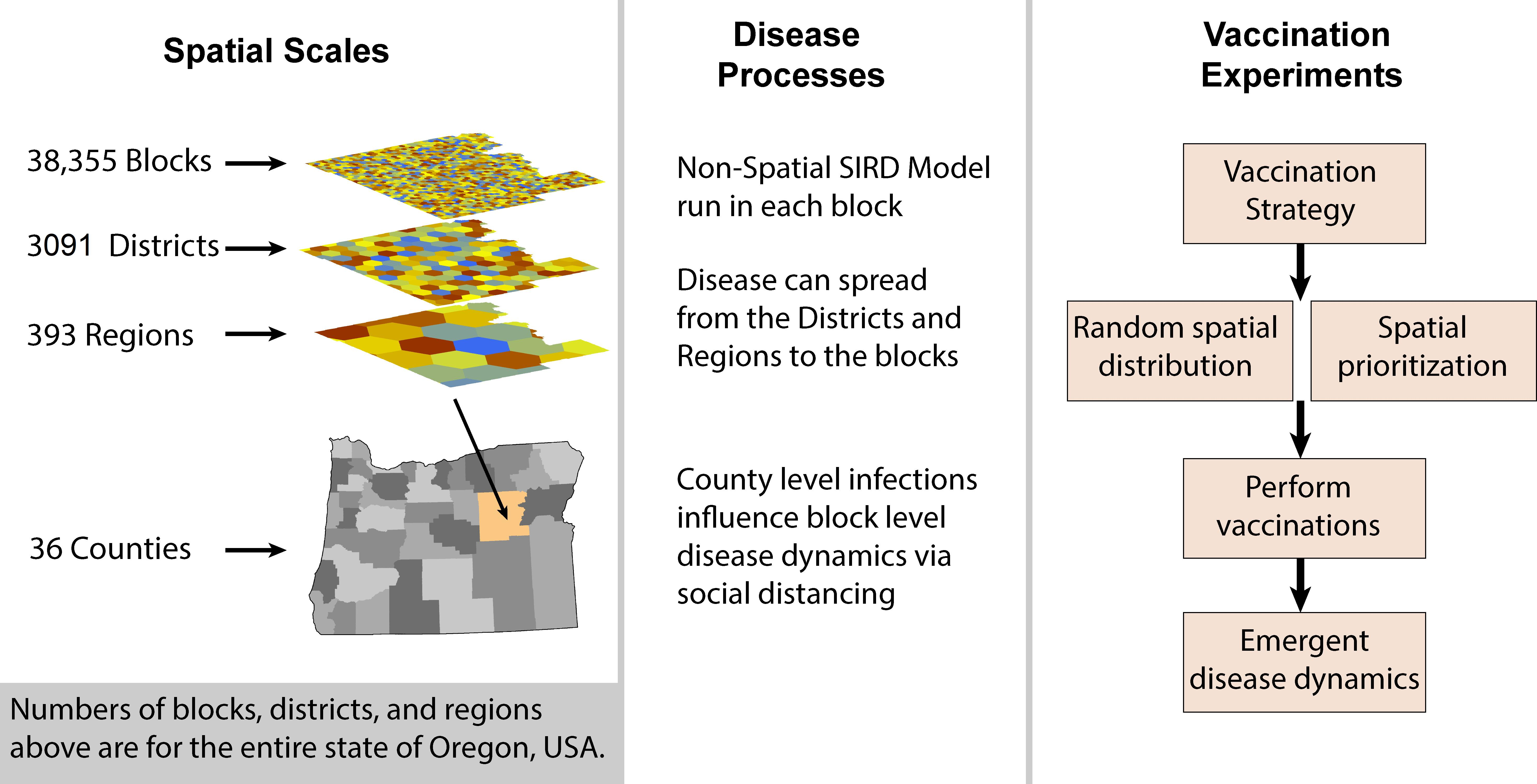
| Scale | Quantity | Max Area (Hexagons) | Max Area (Hectares) |
|---|---|---|---|
| Block | 38,355 | 37 | 800 |
| District | 3091 | 397 | 8600 |
| Region | 393 | 3367 | 73,000 |
| County | 36 | 123,809 | 2.7 M |
| Model Input | Description | Value |
|---|---|---|
| Spatial Data | Population Size | Number per hexagon |
| Patch Maps | Blocks | |
| District | ||
| Regions | ||
| Counties | ||
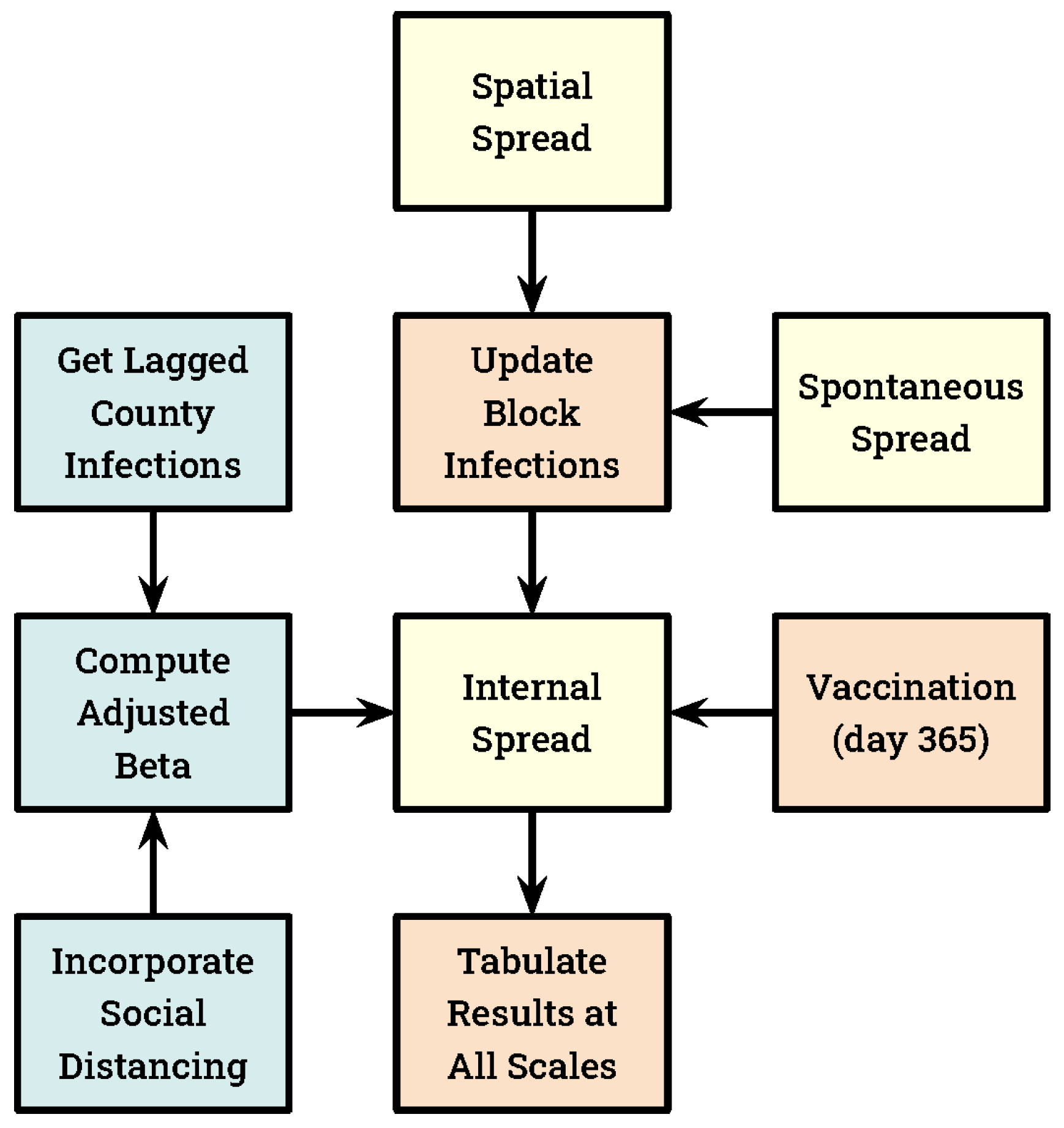
| SIRD Rates | β (infection) | 0.25 |
| γ (recovery) | 0.064 | |
| δ (death) | 0.01 | |
| Spontaneous Infection Rate | Daily rate at which blocks are seeded with a new infection, converting one susceptible individual into an infected. | 1.0 × 10⁻⁷ |
| Adjusted Beta | The model simulates social distancing by replacing β with a smaller value we refer to as “adjusted β”. CI is the lagged infections per 1000 individuals, computed by county. SD, our social distancing coefficient, was set equal to 2.0. | |
| Vaccination | Statewide total | 3 million |
| Acquired immunity rate | 100% |
| Title | Vaccination Strategy | Deployment Strategy |
|---|---|---|
| VUR | Unprioritized | Random |
| VUU | Uniform | |
| VPC | Prioritized | County |
| VPR | Region | |
| VPD | District |
Publisher’s Note: MDPI stays neutral with regard to jurisdictional claims in published maps and institutional affiliations. |
© 2021 by the authors. Licensee MDPI, Basel, Switzerland. This article is an open access article distributed under the terms and conditions of the Creative Commons Attribution (CC BY) license (https://creativecommons.org/licenses/by/4.0/).
Share and Cite
Schumaker, N.H.; Watkins, S.M. Adding Space to Disease Models: A Case Study with COVID-19 in Oregon, USA. Land 2021, 10, 438. https://doi.org/10.3390/land10040438
Schumaker NH, Watkins SM. Adding Space to Disease Models: A Case Study with COVID-19 in Oregon, USA. Land. 2021; 10(4):438. https://doi.org/10.3390/land10040438
Chicago/Turabian StyleSchumaker, Nathan H., and Sydney M. Watkins. 2021. "Adding Space to Disease Models: A Case Study with COVID-19 in Oregon, USA" Land 10, no. 4: 438. https://doi.org/10.3390/land10040438
APA StyleSchumaker, N. H., & Watkins, S. M. (2021). Adding Space to Disease Models: A Case Study with COVID-19 in Oregon, USA. Land, 10(4), 438. https://doi.org/10.3390/land10040438