Article

Adding Space to Disease Models: A Case Study with COVID-19 in Oregon, USA

by
Nathan H. Schumaker
1,* and
Sydney M. Watkins
2
1
Department of Fisheries and Wildlife, Oregon State University Corvallis, Corvallis, OR 97331, USA
2
Computational Ecology Group, Canmore, AB T1W 3L4, Canada
*
Author to whom correspondence should be addressed.
Land 2021, 10(4), 438; https://doi.org/10.3390/land10040438
Submission received: 24 March 2021 / Revised: 15 April 2021 / Accepted: 17 April 2021 / Published: 20 April 2021
(This article belongs to the Section Landscape Ecology)

Abstract

:
We selected the COVID-19 outbreak in the state of Oregon, USA as a system for developing a general geographically nuanced epidemiological forecasting model that balances simplicity, realism, and accessibility. Using the life history simulator HexSim, we inserted a mathematical SIRD disease model into a spatially explicit framework, creating a distributed array of linked compartment models. Our spatial model introduced few additional parameters, but casting the SIRD equations into a geographic setting significantly altered the system’s emergent dynamics. Relative to the non-spatial model, our simple spatial model better replicated the record of observed infection rates in Oregon. We also observed that estimates of vaccination efficacy drawn from the non-spatial model tended to be higher than those obtained from models that incorporate geographic variation. Our spatially explicit SIRD simulations of COVID-19 in Oregon suggest that modest additions of spatial complexity can bring considerable realism to a traditional disease model.

Graphical Abstract

1. Introduction

Disease spread is an inherently spatial process [1,2,3,4,5,6], yet many epidemiological models are non-spatial or pseudo-spatial [7]. This discrepancy reflects the fact that representing explicit spatial structures and nuanced spatiotemporal feedback mechanisms within mathematical and computer models is difficult. Yet, landscape structure clearly influences disease dynamics. Exposure involves the exchange of pathogens between individuals, or an individual and its environment, thus tying rates of infection to population distribution and movement behavior [8,9,10,11]. Furthermore, population-wide emergent properties affecting these processes, such as occupancy rates and source-sink patterns, exhibit complex spatial structures of their own [12,13,14,15,16]. Likewise, the consequences of infection will vary depending on where transmission occurs [17,18]; introducing a novel pathogen into a densely populated area would be more likely to result in an outbreak than if the infection arose in a location with few occupants [19,20]. These concerns, and widespread interest in the role geography plays in disease dynamics, have fueled the development of specialized and highly sophisticated mathematical and computer models [21,22,23,24,25].
Advanced mathematical models can be difficult to understand, and have limited ability to represent dynamic spatial processes operating within complex landscapes [26,27,28,29]. Similarly, while a large and impressive body of work has introduced geographic realism to epidemiological simulators [5,22,30,31], only a fraction of readers encountering these studies have sufficient familiarity with the software employed to fully appreciate key mechanics and assumptions. Here, we illustrate an epidemiological application of HexSim, a simulation model development framework from landscape ecology. HexSim emphasizes generality, flexibility, and accessibility; models constructed within the program may range from non-spatial to spatial, mathematical to individual-based, and from probabilistic to mechanistic [16]. We believe HexSim offers epidemiologists a new development platform that can help balance simplicity and transparency with nuance and realism.
Many mathematical and simulation models of COVID-19 have recently been developed [32,33,34,35,36,37], but few are spatially explicit [29,38]. The principal focus of these models has been to forecast rates of infection and mortality. But these less spatially informed models have limited ability to capture disease dynamics or intervention efforts that vary significantly from place to place. Here, we use COVID-19 as a system for exploring how public health expectations might change as geographic information is introduced to forecasting models. To this end, our study uses both non-spatial and spatial SIRD models to contrast the forecasted benefits of hypothetical vaccine strategies. We begin by describing our modeling system, then demonstrate that it can approximate observed patterns of viral spread in Oregon, and finally employ the tool to explore differences between spatially nuanced vaccination deployment strategies.

2. Materials and Methods

We selected the state of Oregon, USA as a case study location (Figure 1). Oregon, located on the US west coast, is 25 million ha in area and has a population size of 4.2 million. We developed our spatial COVID simulation within the HexSim modeling environment [16]. HexSim models typically follow every individual in one or more populations as they transition through a complex sequence of life history events [39]. In contrast, we designed our COVID simulator as a spatial compartment model in which individuals are only used for tabulating the number of susceptible, infected, recovered, and deceased present at specific locations throughout the landscape [40,41]. Compartment models have been frequently used to improve model accuracy while minimizing complexity [42,43,44].
HexSim (www.hexsim.net accessed on 24 March 2021) is an established application that has contributed to a large number of research papers, primarily in the fields of landscape ecology and conservation biology. Because HexSim does not impose a fixed set of required parameters, model designs may reflect data availability. Though it is well-suited for exploring theory [16,45,46], HexSim is frequently used in applied studies such as population viability analyses [47]. HexSim simulations can include one or more species and are built around user-specified event sequences. It is straightforward to develop species–landscape and species–species interactions, and many HexSim events can be directly linked to spatial patterns and processes. HexSim includes a full genetics sub-model, and simulated individuals may possess any number of life history traits. HexSim’s trait structure and flexible use of space make it ideal for modeling disease systems.
We took advantage of HexSim features to simultaneously track disease dynamics within four distinct map-based units of organization [15,16,48]. HexSim landscapes are tessellated with hexagonal cells, and our models used multi-hexagon, space-filling structures we labeled blocks, districts, regions, and counties to influence disease dynamics at multiple scales (Table 1, Figure 1). Note that, while blocks, districts, and regions are themselves hexagonal in shape, they are assembled from collections of individual HexSim hexagonal cells and will always be referred to by name; subsequent use of the term hexagon will imply the individual hexagonal cells from which these larger structures are assembled. Our model represented the state of Oregon using 1,173,651 hexagons, each of which was 21.65 ha in area and 500 m in width (between parallel sides). Individual blocks (800 ha), districts (8600 ha), and regions (73,000 ha) were roughly one order of magnitude different in size. While blocks, districts, and regions represent arbitrary spatial units, our county delineations correspond to the state’s actual administrative boundaries.
Our smaller spatial structures could be split across larger ones, for example, a block might be spread across two districts and a district might span two or more regions. Blocks, districts, and regions intersected by the Oregon boundary were clipped so that they fell entirely within the state, thus making them smaller in size. The district and regional scales formed part of a mechanism for spreading local infections between neighboring blocks. We ran a SIRD model separately in each block, as defined by the following equations:
S ( t ) = S ( t 1 ) β N S ( t 1 ) I ( t 1 )
I ( t ) = I ( t 1 ) + β N S ( t 1 ) I ( t 1 ) γ I ( t 1 ) δ I ( t 1 )
R ( t ) = R ( t 1 ) + γ I ( t 1 )
D ( t ) = D ( t 1 ) + δ I ( t 1 )
S, I, R, and D refer to the numbers of susceptible, infected, recovered, and deceased individuals within a block. N denotes a block’s total population size, which the model obtained using a statewide map of population densities. Our density map recorded the number of individuals per hexagon, for all hexagons across the state. These density values ranged from zero to 2677 individuals per hexagon. β is the infection rate, γ is the recovery rate, and δ is the death rate. Because parameter values were not available for Oregon, we used estimates of β = 0.25, γ = 0.064, and δ = 0.01 in our model. These three parameter values (Table 2) were taken from the few existing COVID-19 studies presently available that utilized discrete time SIRD models [33,34,49]. When our model begins, we initialize each block with the values S = N and I = R = D = 0. We used a time step (t) of one day and ran our simulations for two years. Our model includes a mechanism that simulates the introduction of infections from outside the system (see below), which is how disease outbreaks were initiated.
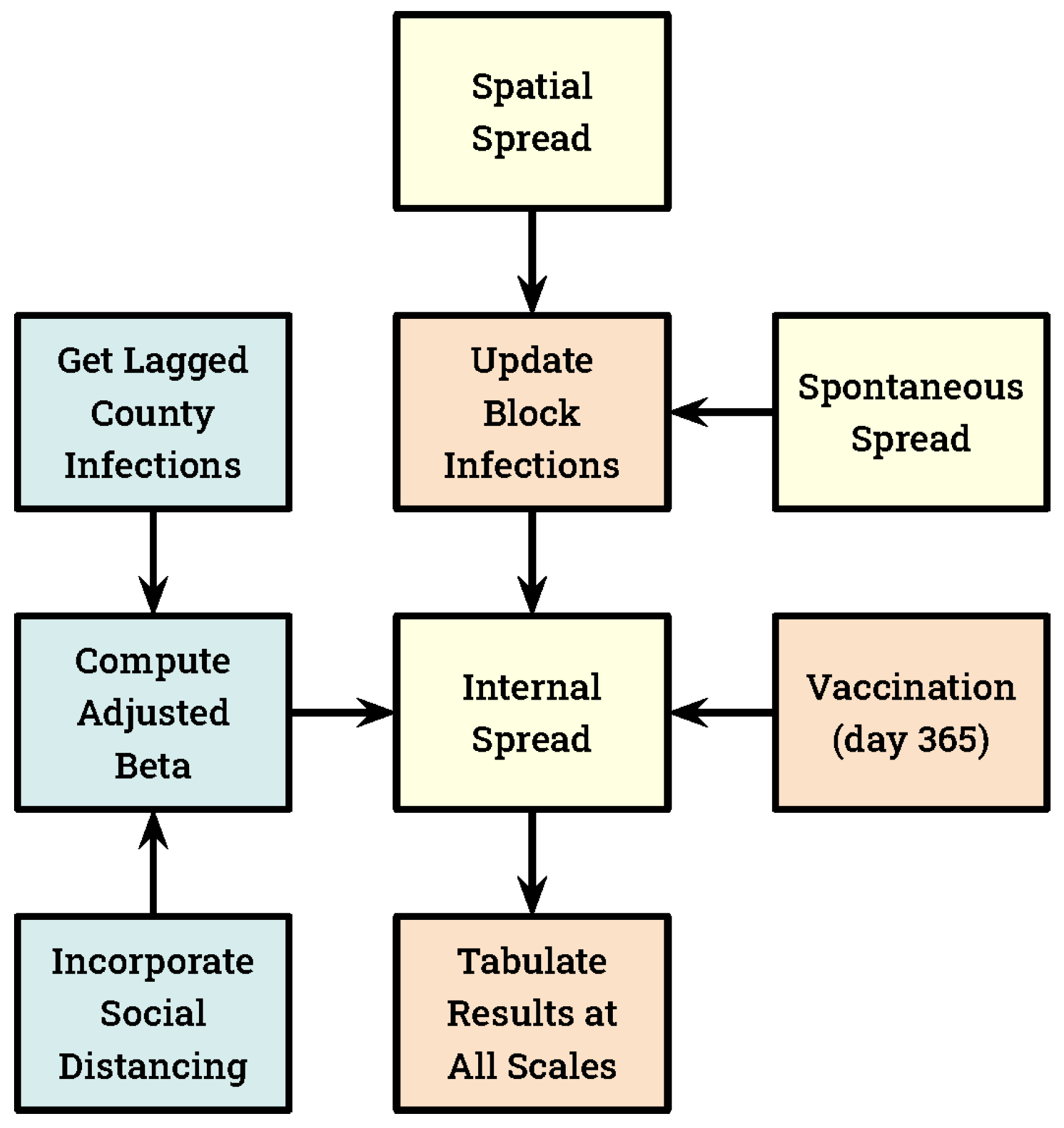
Our model couples three disease spread mechanisms (Figure 2). We refer to changes in the number of infected individuals resulting from the susceptible, infected, recovered, and diseased (SIRD) calculations as internal spread because they were computed independently within each block. We separately initiated new infections in blocks based upon the number of infections present in the districts and regions within which they were embedded. We refer to this exchange of infections between blocks and their neighborhoods as spatial spread. Our spatial spread mechanism, which is invariant to changes in the number, size, and distribution of districts and regions, proceeded as follows. First, the number of infections within each district and region were acquired by summing the infections present in the blocks they overlapped. Because blocks are multi-hexagon areas, these sums were taken at an individual hexagon scale, allowing a block’s infections to be split across adjacent districts or regions. Districts and regions then contributed infections back to the blocks they contain at a rate equal to their respective sizes. To avoid double-counting, the spatial spread from a district to a block ignored that block’s contribution to the district. Likewise, the spatial spread from a region to a block discounted the contribution already made to the block by districts that fell within that region. Our spatial spread mechanism may be thought of as somewhat similar to a moving-window smoothing operator, except that it ran at two spatial scales simultaneously.
Our models include a third mechanism for introducing infections to blocks, which we refer to as spontaneous spread. Each day, all blocks received a single new infection with a probability equal to their population size × 10−7. Thus, on average, a block with 1000 inhabitants would experience one spontaneous infection every 27.4 years. Statewide, this process yielded approximately one new spontaneous infection every 2.4 days. The rate coefficient (10−7) employed here was an approximation based upon minimal available empirical evidence.
Our social distance mechanism assumes that numbers of infections are reported at the county scale, and that people become more cautious as infection rates increase. We imposed social distancing by lowering the value of β in the SIRD equations based on the simulated number of infections present in the county within which each block was located. We refer to these reduced β values as adjusted β, hereafter written βadj. For these calculations, we used the number of infections present in a county two weeks prior to the day for which βadj was required. This lag period was intended to account for delays between infection and the onset of symptoms, and between testing and the reporting of results. Blocks that straddled counties used a multi-county mean value for the number of lagged infections. βadj was derived from the infection data using a piecewise linear function as follows. Let CI represent the county-wide lagged infections per 1000 individuals, and SD represent our social distancing coefficient. When CI fell between 0 and SD, βadj was computed as
β a d j = β ( 1 C I S D )
when CI exceeded SD, βadj was set to zero. Because data were not available to parameterize our social distancing mechanism, we adjusted the SD coefficient to produce an emergent mean statewide number of cumulative infections equal to twice the observed value at simulation day 200, thus attempting to account for the pervasive lack of COVID testing [44]. Oregon recorded 29,337 COVID-19 infections on day 200 of the state’s epidemic [50]. Our assumption that actual infections exceeded documented cases by a factor of two constituted a plausible conservative estimate. Subsequent evidence has suggested this estimate is likely low [51]. We also used this SD coefficient in our non-spatial social distancing models (described below). Simulation day 200 preceded vaccination in our study.
We developed five vaccination strategies, which fell into two general classes titled unprioritized and prioritized (Table 3). All vaccinations were implemented at the block scale, for simplicity were performed entirely on simulation day 365, and were assumed to impart complete immunity. Both susceptible and recovered classes were eligible for vaccination. Regardless of strategy, our vaccination target was always 3 million individuals, equivalent to 71% of the state’s population. We selected this target value because 70% is frequently considered a lower bound for achieving herd immunity in large populations. Our three prioritized vaccination strategies were performed iteratively, one block at a time, until the vaccination target was reached. Our two unprioritized strategies involved either vaccinating blocks at random until the target was reached (VUR) or dividing the target number of vaccinations across all blocks proportional to their population size (VUU).
Our three prioritized strategies involved identification of the districts (VPD), regions (VPR), or counties (VPC) with the greatest number of current infections, and the subsequent vaccination of some or all blocks that fell within them. These strategies utilized a pair of nested iterative loops. The outer loop selected the county, region, or district with the most infections, while the inner loop randomly selected blocks within this area and vaccinated their entire eligible population. The inner loop terminated when all blocks had been vaccinated, or if the vaccination target was met. When the inner loop completed before the vaccination target was reached, the outer loop proceeded to the next most infected district, region, or county. In contrast to the two unprioritized vaccination strategies, our three prioritized strategies were intended to generate clustered vaccination patterns.
In summary, disease spread in our spatial models resulted from running the SIRD equations at the block scale (internal spread). However, infections were also introduced into blocks from the districts and regions in which they were located, at a rate set equal to their relative sizes (spatial spread). Finally, infections were added to blocks probabilistically in order to simulate the exchange of individuals from outside local neighborhoods (spontaneous spread). We developed seven spatial models, five of which included vaccination and social distancing (Table 3). Of the two spatial models without vaccination, one included social distancing and the other did not.
We used three non-spatial SIRD models as a reference for measuring the influence that geographic detail had on simulated COVID dynamics. These included the SIRD equations alone, the SIRD equations with social distancing, and the SIRD equations with both social distancing and vaccination. All models were developed in HexSim, and the input data required to run them is summarized in Table 2. We ran ten replicate simulations of each model, and we report below on the mean values taken across these replicates.

3. Results

As described above, we parameterized our spatial model given an assumption that the cumulative number of infections at simulation day 200 should be twice the officially recorded value. Our single tuning parameter was a social distancing coefficient (SD). The spatial model with social distancing met this target when SD was set to 2.0. We used this value for SD in all of the non-spatial and spatial simulations that incorporated social distancing.
In the absence of social distancing and vaccination, our non-spatial SIRD model produced a single huge pulse of infections reaching a maximum of 1.5 M cumulative infections by day 100. At this time, the number of new infections dropped rapidly to zero and remained there. When social distancing was added, the non-spatial model exhibited stable oscillations with peak numbers of new infections separated by roughly 30 days, and on average >200 new infections per day at steady-state. When vaccination was added to this model (on day 365), the number of subsequent new infections dropped to zero, suggesting that herd immunity had been achieved. This non-spatial model with both social distancing and vaccination produced approximately 90K cumulative infections over the two-year simulation time frame.
In the absence of social distancing and vaccination, our spatial SIRD model also produced a single large pulse of infections, but this outbreak was distributed over a period of roughly 200 days, with a cumulative maximum of 1.75 M infected individuals. When social distancing was added to this model, the number of new infections became cyclic (Figure 3), with the same period as was observed in the non-spatial model. After relatively small initial outbreak, subsequent cycles ranged between roughly 100 and 400 new infections per day (2.37 to 9.48 per 100 K) statewide.
The VUR deployment strategy (Table 3) produced the least benefit of our five spatial vaccination experiments (Figure 4). Under this strategy, the number of new infections per day remained quite large at times. In contrast, the VUU deployment strategy exhibited the greatest vaccination efficacy. Under the VUU strategy, daily new infections fell to roughly four individuals for much of the final simulation year. Our three prioritized vaccination deployment strategies (VPC, VPR, and VPD) produced a number of new infections ranging between 40 and 130 per day (Figure 4).
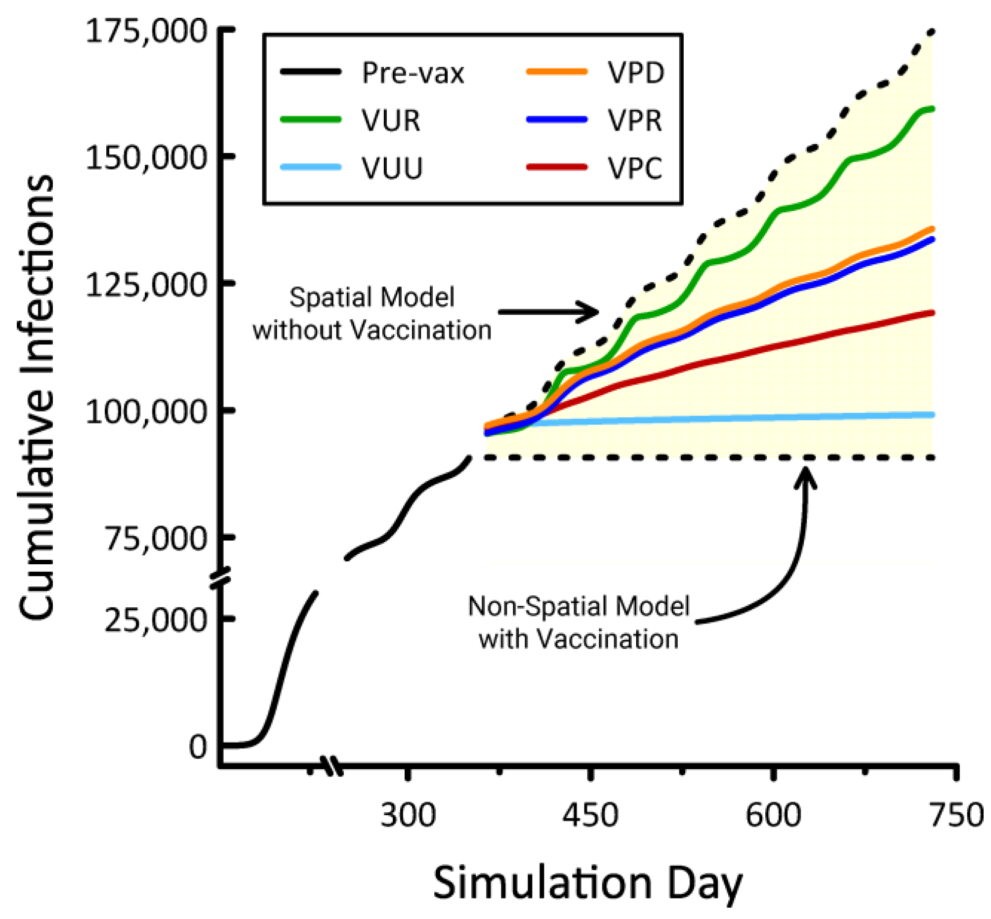
Trends in cumulative infections resulting from our vaccination scenarios were bounded below by the results from the non-spatial model with vaccination and above by the spatial model without vaccination (Figure 5). Both of these models included social distancing. In the case of the non-spatial model with vaccination, herd immunity was achieved and new infections ceased. In the spatial model without vaccination, new infections accumulated steadily but at a rate that would preclude reaching herd immunity for decades. The non-spatial model (Equations (1)–(4) applied to the entire state) necessarily assumes the perfect mixing of individuals, and Figure 5 suggests that vaccination is maximally efficacious in such artificially connected populations. In contrast, the lack of connectivity exhibited by our spatial models inhibits viral spread, shifting the disease dynamic from a pattern of explosive growth and decline to one of longer-term persistence. Figure 5 also indicates that, in the absence of vaccination, spatially distributed populations are capable of sustaining high infection rates for extended periods. When vaccination was prioritized by counties (VPC), regions (VPR), and districts (VPD), observed benefits fell between the most effective (VUU) and least effective (VUR) scenarios. Efficacy increased with the size of the areas within which vaccinations were prioritized.
All of our vaccination scenarios involved instantly inoculating a majority (71%) of the overall population. When prioritizing by county, we observed a range of 8–11 counties were selected for vaccination, depending on the replicate. These selections accounted for 14.6 to 20.1% of the total state area. When prioritized by region and district, the areas selected for vaccination comprised 5.6 to 6.8% and 3.5 to 5.1% of the state, respectively (Figure 6). Under the VUR strategy, roughly 71% of blocks were vaccinated entirely, with the remainder left untreated. In contrast, the VUU strategy partially treated every block. The geographic distributions of these unprioritized vaccination schemes were unremarkable, with VUR generating random patterns and VUU producing uniform coverage statewide.

4. Discussion

Through the addition of space, we were able to represent three complementary and interacting routes to infection. The SIRD model governed internal spread, resulting from disease dynamics within individual blocks. We also simulated a process termed spatial spread, in which local neighborhoods contributed infections to blocks that fell within them. Our use of both districts and regions to define neighborhoods helped to eliminate artifacts that result from sampling spatially-distributed processes at a single scale [16]. Finally, we used a probabilistic mechanism called spontaneous spread to capture disease introduction from outside of a block’s neighborhood. Our approach illustrates how a traditional non-spatial epidemiological model can be cast into a geographic framework without imposing significant additional complexity or parameters.
Oregon experienced a dramatic lack of COVID testing in the early months of the pandemic [52,53,54], and we parameterized our model under the assumption that the actual number of infections was twice the value recorded on the outbreak’s 200th day. Thus calibrated, our spatial simulations produced emergent rates and patterns of disease spread that were plausible given the simplicity of our underlying SIRD model [50,55] and the absence of data necessary to link social distancing to behavioral trends. This assessment is reinforced by the huge discrepancies observed when results from our nonspatial and non-social distanced models are compared to state records. Our simulation models exhibited a rapid initial increase in COVID cases that is not mirrored in published state tallies (Figure 3), but this discrepancy was consistent with the highly limited availability of testing during the pandemic’s first few months and with this disease’s observed rates of spread in other parts of the world. By day 100, observed and simulated numbers of new COVID cases per day were in better agreement. Our model failed to predict the large outbreak that began during the 2020 holiday season, but it could have approximated this surge had we allowed the state’s cultural geography to influence social distancing.
By comparing our non-spatial and spatial models with and without social distancing and vaccination, we confirmed that introducing geographic detail can characteristically alter emergent model properties. For example, while our non-spatial SIRD model suggests that vaccinating 71% of the population is sufficient to achieve herd immunity in Oregon, none of our spatial models support this conclusion. Among the spatial models, the closest approximation to herd immunity was realized from the VUU scenario, which drove new infections down to roughly four per day. Our three prioritized vaccination deployment strategies (VPC, VPR, and VPD) lowered the number of new infections to between 40 and 130 per day. This benefit should be viewed in the context of our spatial non-vaccination model’s forecast of approximately 400 new infections per day at steady-state.
The majority of Oregon’s population is located within the Willamette Valley, which extends from Portland in the north to Eugene in the south. This human geography explains the character of the vaccination patterns emerging from our three prioritized strategies (Figure 6). Based purely on logistics, less effort would be involved in vaccinating smaller areas having denser populations composed of a more receptive populace. From this standpoint, our VUU scenario would be the least realistic vaccination strategy. This suggests that practical vaccination deployment strategies are unlikely to achieve efficacy goals established based on insights gleaned from simple non-spatial models. Our results indicate that fully vaccinating large geographic areas yields a maximum benefit, but this outcome is diminished when even small population fragments are left unvaccinated.
We intentionally limited the complexity of mechanisms and number of parameters in our HexSim COVID models (Table 2). For example, we assumed that βadj (CI) was piecewise linear with βadj (0) = β and βadj (≥ 2) = 0, where CI represented the lagged number of county infections per 1000 individuals. This relationship could easily be replaced with a nonlinear function having a nonzero intercept. Likewise, a more customizable mechanism (e.g., a gravity model [56,57,58]) could be substituted in place of the spontaneous disease spread process, and our simplification that ensured every susceptible individual in a chosen block was vaccinated could easily be made more realistic. HexSim facilitates more substantive enhancements to model realism as well. For example, independent agents could be readily added to our compartment model superstructure. Doing so would create avenues for linking dynamic individual behaviors and conditions to rates of transmission, exposure, and outcomes. In addition, most HexSim processes can be influenced by multiple dynamic geographic datasets, including maps developed on-the-fly from model state. This encourages the incorporation of realistic feedback mechanisms that vary across both space and time.
Our models’ assumption that vaccination is perfectly effective could easily be made more realistic. Doing so would simply involve adding a probabilistic term to the post-vaccination transition from the susceptible to recovered classes. In addition, it would be straightforward to allow individuals to transition from the recovered class back to susceptible. With time, better estimates of the SIRD model parameters themselves will become available, making it possible to improve the model’s fit to existing data. Critically, our model’s design, and particularly its implementation within HexSim, allows for myriad enhancements that vary social distancing across both space and time, or that simulate public health mandates such as quarantines and lockdowns. While our spatial models with social distancing already dramatically outperformed their simple mathematical counterparts, improvements such as these would add greatly to the model’s realism and its utility as a forecasting tool.
Our HexSim case study illustrates that a modest investment in spatial detail can greatly enhance a traditional mathematical disease model. We believe the methods described here strike a useful balance between simplicity, realism, and accessibility, while also reinforcing the importance of linkages between landscape ecology and epidemiology. HexSim’s extensive graphical user interface, trait structure, life history events, and facilities for linking events to mapped data make our models easy to understand and straightforward to modify.

5. Conclusions

We have used the epidemic of COVID-19 in the state of Oregon, USA, as a case study to demonstrate that a traditional mathematical disease model can be embedded within a spatially explicit framework with the addition of few novel parameters. While our simple model’s fit to existing trends is imperfect, it dramatically outperformed analogous models that did not incorporate space or social distancing. Our model framework is highly transferable and extensible, being both easily repurposed for other locations or disease systems and readily enhanced through the introduction of further realism, spatial detail, and temporal dynamics. We hope this case study encourages other researchers to explore and adopt these accessible tools and methods for investigating spatial disease dynamics, and we assert that our HexSim modeling environment will prove itself even more valuable as these scientific challenges increase in scope and complexity.
In spite of the limitations described above, we were able to exploit our model to develop hypotheses with relevance to public health. It follows from our case study that traditional nonspatial disease models are likely to underestimate the number of vaccinations necessary to achieve herd immunity in a large population. Furthermore, our analysis goes on to illustrate that the effort necessary to control a pathogen like COVID-19 will likely vary depending on the spatial patterns of vaccine distribution. We encourage others to build on our work by adapting these methods to different systems. In particular, we encourage graduate students to explore these tools and examine our techniques. The cost to entry will be low, and the potential for exciting new research contributions is high.

Author Contributions

Both authors contributed equally to this research paper. Both authors have read and agreed to the published version of the manuscript.

Funding

This research received no external funding.

Data Availability Statement

The models described here can be downloaded from the HexSim website, www.hexsim.net, accessed on 24 March 2021.

Acknowledgments

We are grateful to Julie Heinrichs and Paul Severns for many inspiring discussions, providing insights, and reviewing our draft manuscripts. We are also indebted to Marc Weber for providing the Oregon population density map that we used in our model, and to two anonymous reviewers.

Conflicts of Interest

The authors declare no conflict of interest.

References

  1. Belik, V.; Geisel, T.; Brockmann, D. Natural Human Mobility Patterns and Spatial Spread of Infectious Diseases. Phys. Rev. X 2011, 1. [Google Scholar] [CrossRef] [Green Version]
  2. Hagenaars, T.; Donnelly, C.; Ferguson, N. Spatial heterogeneity and the persistence of infectious diseases. J. Theor. Biol. 2004, 229, 349–359. [Google Scholar] [CrossRef] [PubMed]
  3. Kraemer, M.U.G.; Faria, N.R.; Reiner, R.C.; Golding, N.; Nikolay, B.; Stasse, S.A.; Johansson, M.; Salje, H.; Faye, O.; Wint, G.R.W.; et al. Spread of yellow fever virus outbreak in Angola and the Democratic Republic of the Congo 2015–2016: A modelling study. Lancet Infect. Dis. 2017, 17, 330–338. [Google Scholar] [CrossRef]
  4. Ostfeld, R.S.; Glass, G.E.; Keesing, F. Spatial epidemiology: An emerging (or re-emerging) discipline. Trends Ecol. Evol. 2005, 20, 328–336. [Google Scholar] [CrossRef] [PubMed]
  5. Riley, S. Large-Scale Spatial-Transmission Models of Infectious Disease. Science 2007, 316, 1298–1301. [Google Scholar] [CrossRef] [Green Version]
  6. Sun, G.-Q.; Jusup, M.; Jin, Z.; Wang, Y.; Wang, Z. Pattern transitions in spatial epidemics: Mechanisms and emergent properties. Phys. Life Rev. 2016, 19, 43–73. [Google Scholar] [CrossRef] [Green Version]
  7. Jacquez, G.M. Spatial analysis in epidemiology: Nascent science or a failure of GIS? J. Geogr. Syst. 2000, 2, 91–97. [Google Scholar] [CrossRef]
  8. Dalziel, B.D.; Pourbohloul, B.; Ellner, S.P. Human mobility patterns predict divergent epidemic dynamics among cities. Proc. Proc. R. Soc. B Biol. Sci. 2013, 280, 20130763. [Google Scholar] [CrossRef] [PubMed]
  9. Merler, S.; Ajelli, M. The role of population heterogeneity and human mobility in the spread of pandemic influenza. Proc. R. Soc. B Biol. Sci. 2010, 277, 557–565. [Google Scholar] [CrossRef] [PubMed] [Green Version]
  10. Onozuka, D.; Hagihara, A. Spatial and Temporal Dynamics of Influenza Outbreaks. Epidemiology 2008, 19, 824–828. [Google Scholar] [CrossRef] [PubMed]
  11. Wesolowski, A.; Eagle, N.; Tatem, A.J.; Smith, D.L.; Noor, A.M.; Snow, R.W.; Buckee, C.O. Quantifying the Impact of Human Mobility on Malaria. Science 2012, 338, 267–270. [Google Scholar] [CrossRef] [PubMed] [Green Version]
  12. Lloyd, A.L.; May, R.M. Spatial Heterogeneity in Epidemic Models. J. Theor. Biol. 1996, 179, 1–11. [Google Scholar] [CrossRef]
  13. Pulliam, H.R. Sources, Sinks, and Population Regulation. Am. Nat. 1988, 132, 652–661. [Google Scholar] [CrossRef]
  14. Pickett, S.T.A.; Cadenasso, M.L. Landscape Ecology: Spatial Heterogeneity in Ecological Systems. Science 1995, 269, 331–334. [Google Scholar] [CrossRef]
  15. Schumaker, N.H.; Brookes, A.; Dunk, J.R.; Woodbridge, B.; Heinrichs, J.A.; Lawler, J.J.; Carroll, C.; LaPlante, D. Mapping sources, sinks, and connectivity using a simulation model of northern spotted owls. Landsc. Ecol. 2014, 29, 579–592. [Google Scholar] [CrossRef]
  16. Schumaker, N.H.; Brookes, A. HexSim: A modeling environment for ecology and conservation. Landsc. Ecol. 2018, 33, 197–211. [Google Scholar] [CrossRef]
  17. Legrand, J.; Grais, R.F.; Boelle, P.-Y.; Valleron, A.-J.; Flahault, A. Understanding the dynamics of Ebola epidemics. Epidemiol. Infect. 2006, 135, 610–621. [Google Scholar] [CrossRef] [PubMed]
  18. Merler, S.; Ajelli, M.; Fumanelli, L.; Gomes, M.F.C.; Piontti, A.P.Y.; Rossi, L.; Chao, D.L.; Longini, I.M.; Halloran, M.E.; Vespignani, A. Spatiotemporal spread of the 2014 outbreak of Ebola virus disease in Liberia and the effectiveness of non-pharmaceutical interventions: A computational modelling analysis. Lancet Infect. Dis. 2015, 15, 204–211. [Google Scholar] [CrossRef] [Green Version]
  19. Kraemer, M.U.G.; Perkins, T.A.; Cummings, D.A.T.; Zakar, R.; Hay, S.I.; Smith, D.L.; Reiner, R.C. Big city, small world: Density, contact rates, and transmission of dengue across Pakistan. J. R. Soc. Interface 2015, 12, 20150468. [Google Scholar] [CrossRef] [PubMed] [Green Version]
  20. Wesolowski, A.; Zu Erbach-Schoenberg, E.; Tatem, A.J.; Lourenço, C.; Viboud, C.; Charu, V.; Eagle, N.; Engø-Monsen, K.; Qureshi, T.; Buckee, C.O.; et al. Multinational patterns of seasonal asymmetry in human movement influence infectious disease dynamics. Nat. Commun. 2017, 8, 1–9. [Google Scholar] [CrossRef] [PubMed]
  21. Bian, L. A conceptual framework for an individual-based spatially explicit epidemiological model. Environ. Plan. B Plan. Des. 2004, 31, 381–395. [Google Scholar] [CrossRef] [Green Version]
  22. Chowell, G.; Rothenberg, R. Spatial infectious disease epidemiology: On the cusp. BMC Med. 2018, 16, 1–5. [Google Scholar] [CrossRef] [PubMed] [Green Version]
  23. Elliott, P.; Wartenberg, D. Spatial Epidemiology: Current Approaches and Future Challenges. Environ. Health Perspect. 2004, 112, 998–1006. [Google Scholar] [CrossRef]
  24. Kirby, R.S.; Delmelle, E.; Eberth, J.M. Advances in spatial epidemiology and geographic information systems. Ann. Epidemiol. 2017, 27, 1–9. [Google Scholar] [CrossRef]
  25. Meentemeyer, R.K.; Haas, S.E.; Václavík, T. Landscape Epidemiology of Emerging Infectious Diseases in Natural and Human-Altered Ecosystems. Annu. Rev. Phytopathol. 2012, 50, 379–402. [Google Scholar] [CrossRef] [PubMed] [Green Version]
  26. Getz, W.M.; Salter, R.; Muellerklein, O.; Yoon, H.S.; Tallam, K. Modeling epidemics: A primer and Numerus Model Builder implementation. Epidemics 2018, 25, 9–19. [Google Scholar] [CrossRef]
  27. Kelsall, J.; Wakefield, J. Modeling Spatial Variation in Disease Risk. J. Am. Stat. Assoc. 2002, 97, 692–701. [Google Scholar] [CrossRef]
  28. Morato, M.M.; Bastos, S.B.; Cajueiro, D.O.; Normey-Rico, J.E. An optimal predictive control strategy for COVID-19 (SARS-CoV-2) social distancing policies in Brazil. Annu. Rev. Control 2020, 50, 417–431. [Google Scholar] [CrossRef]
  29. Roques, L.; Bonnefon, O.; Baudrot, V.; Soubeyrand, S.; Berestycki, H. A Parsimonious Model for Spatial Transmission and Heterogeneity in the COVID-19 Propagation. arXiv 2020, arXiv:2007.08002. [Google Scholar]
  30. Balcan, D.; Colizza, V.; Gonçalves, B.; Hu, H.; Ramasco, J.J.; Vespignani, A. Multiscale mobility networks and the spatial spreading of infectious diseases. Proc. Natl. Acad. Sci. USA 2009, 106, 21484–21489. [Google Scholar] [CrossRef] [Green Version]
  31. Balcan, D.; Gonçalves, B.; Hu, H.; Ramasco, J.J.; Colizza, V.; Vespignani, A. Modeling the spatial spread of infectious diseases: The GLobal Epidemic and Mobility computational model. J. Comput. Sci. 2010, 1, 132–145. [Google Scholar] [CrossRef] [PubMed] [Green Version]
  32. Chang, S.L.; Harding, N.; Zachreson, C.; Cliff, O.M.; Prokopenko, M. Modelling transmission and control of the COVID-19 pandemic in Australia. Nat. Commun. 2020, 11, 1–13. [Google Scholar] [CrossRef] [PubMed]
  33. Chakraborty, A.; Chen, J.; Desvars-Larrive, A.; Klimek, P.; Flores Tames, E.; Garcia, D.; Horstmeyer, L.; Kaleta, M.; Lasser, J.; Rassish, J.; et al. Analyzing Covid-19 Data Using SIRD Models. medRxiv 2020. MedRxiv 2020.05.28.20115527. [Google Scholar] [CrossRef]
  34. Chatterjee, S.; Sarkar, A.; Chatterjee, S.; Karmakar, M.; Paul, R. Studying the progress of COVID-19 outbreak in India using SIRD model. Indian J. Phys. 2020, 1–17. [Google Scholar] [CrossRef] [PubMed]
  35. Peng, L.; Yang, W.; Zhang, D.; Zhuge, C.; Hong, L. Epidemic Analysis of COVID-19 in China by Dynamical Modeling. arXiv 2020, arXiv:2002.06563. [Google Scholar]
  36. Petropoulos, F.; Makridakis, S. Forecasting the novel coronavirus COVID-19. PLoS ONE 2020, 15, e0231236. [Google Scholar] [CrossRef] [PubMed]
  37. Silva, P.C.; Batista, P.V.; Lima, H.S.; Alves, M.A.; Guimarães, F.G.; Silva, R.C. COVID-ABS: An agent-based model of COVID-19 epidemic to simulate health and economic effects of social distancing interventions. Chaos Solitons Fractals 2020, 139, 110088. [Google Scholar] [CrossRef]
  38. Danon, L.; Brooks-Pollock, E.; Bailey, M.; Keeling, M.J. A Spatial Model of CoVID-19 Transmission in England and Wales: Early Spread and Peak Timing. medRxiv 2020. MedRxiv 2020.02.12.20022566. [Google Scholar] [CrossRef] [Green Version]
  39. Snyder, M.N.; Schumaker, N.H.; Ebersole, J.L.; Dunham, J.B.; Comeleo, R.L.; Keefer, M.L.; Leinenbach, P.; Brookes, A.; Cope, B.; Wu, J.; et al. Individual based modeling of fish migration in a 2-D river system: Model description and case study. Landsc. Ecol. 2019, 34, 737–754. [Google Scholar] [CrossRef]
  40. Heesterbeek, H.; Anderson, R.M.; Andreasen, V.; Bansal, S.; De Angelis, D.; Dye, C.; Eames, K.T.D.; Edmunds, W.J.; Frost, S.D.W.; Funk, S.; et al. Modeling infectious disease dynamics in the complex landscape of global health. Science 2015, 347, aaa4339. [Google Scholar] [CrossRef] [PubMed] [Green Version]
  41. Kermack, W.O.; McKendrick, A.G. A contribution to the mathematical theory of epidemics. Proc. R. Soc. Lond. Ser. A Math. Phys. Sci. 1927, 115, 700–721. [Google Scholar] [CrossRef] [Green Version]
  42. Carletti, T.; Fanelli, D.; Piazza, F. COVID-19: The unreasonable effectiveness of simple models. Chaos Solitons Fractals X 2020, 5, 100034. [Google Scholar] [CrossRef]
  43. Postnikov, E.B. Estimation of COVID-19 dynamics “on a back-of-envelope”: Does the simplest SIR model provide quantitative parameters and predictions? Chaos Solitons Fractals 2020, 135, 109841. [Google Scholar] [CrossRef] [PubMed]
  44. Roda, W.C.; Varughese, M.B.; Han, D.; Li, M.Y. Why is it difficult to accurately predict the COVID-19 epidemic? Infect. Dis. Model. 2020, 5, 271–281. [Google Scholar] [CrossRef] [PubMed]
  45. Heinrichs, J.A.; Lawler, J.J.; Schumaker, N.H. Intrinsic and extrinsic drivers of source–sink dynamics. Ecol. Evol. 2016, 6, 892–904. [Google Scholar] [CrossRef] [PubMed] [Green Version]
  46. Heinrichs, J.A.; Lawler, J.J.; Schumaker, N.H.; Walker, L.E.; Cimprich, D.A.; Bleisch, A. Assessing source-sink stability in the context of management and land-use change. Landsc. Ecol. 2019, 34, 259–274. [Google Scholar] [CrossRef]
  47. Dunk, J.R.; Woodbridge, B.; Schumaker, N.; Glenn, E.M.; White, B.; Laplante, D.W.; Anthony, R.G.; Davis, R.J.; Halupka, K.; Henson, P.; et al. Conservation planning for species recovery under the Endangered Species Act: A case study with the Northern Spotted Owl. PLoS ONE 2019, 14, e0210643. [Google Scholar] [CrossRef]
  48. Barbosa, P.; Schumaker, N.H.; Brandon, K.R.; Bager, A.; Grilo, C. Simulating the consequences of roads for wildlife population dynamics. Landsc. Urban. Plan. 2020, 193, 103672. [Google Scholar] [CrossRef] [PubMed]
  49. Anastassopoulou, C.; Russo, L.; Tsakris, A.; Siettos, C. Data-based analysis, modelling and forecasting of the COVID-19 outbreak. PLoS ONE 2020, 15, e0230405. [Google Scholar] [CrossRef] [Green Version]
  50. The New York Times. Coronavirus (Covid-19) Data in the United States. 2020. Available online: https://github.com/nytimes/covid-19-data (accessed on 15 March 2021).
  51. Lau, H.; Khosrawipour, T.; Kocbach, P.; Ichii, H.; Bania, J.; Khosrawipour, V. Evaluating the massive underreporting and undertesting of COVID-19 cases in multiple global epicenters. Pulmonology 2020, 27, 110–115. [Google Scholar] [CrossRef] [PubMed]
  52. Krantz, S.G.; Rao, A.S.S. Level of underreporting including underdiagnosis before the first peak of COVID-19 in various countries: Preliminary retrospective results based on wavelets and deterministic modeling. Infect. Control Hosp. Epidemiol. 2020, 41, 857–859. [Google Scholar] [CrossRef] [PubMed] [Green Version]
  53. Jagodnik, K.M.; Giorgi, F.M.; Ray, F.; Lachmann, A. Correcting Under-Reported COVID-19 Case Numbers: Estimating the True Scale of the Pandemic. medRxiv 2020. MedRxiv 2020.03.14.20036178. [Google Scholar] [CrossRef] [Green Version]
  54. The Covid Tracking Project at The Atlantic. 2020. Available online: https://covidtracking.com/ (accessed on 15 March 2021).
  55. Covid Act Now. 2020. Available online: https://covidactnow.org/ (accessed on 15 March 2021).
  56. Jandarov, R.; Haran, M.; Bjørnstad, O.; Grenfell, B. Emulating a gravity model to infer the spatiotemporal dynamics of an infectious disease. J. R. Stat. Soc. Ser. C Appl. Stat. 2014, 63, 423–444. [Google Scholar] [CrossRef] [Green Version]
  57. Li, X.; Tian, H.; Lai, D.; Zhang, Z. Validation of the Gravity Model in Predicting the Global Spread of Influenza. Int. J. Environ. Res. Public Health 2011, 8, 3134–3143. [Google Scholar] [CrossRef] [PubMed] [Green Version]
  58. Xia, Y.; Bjørnstad, O.N.; Grenfell, B.T. Measles Metapopulation Dynamics: A Gravity Model for Epidemiological Coupling and Dynamics. Am. Nat. 2004, 164, 267–281. [Google Scholar] [CrossRef]
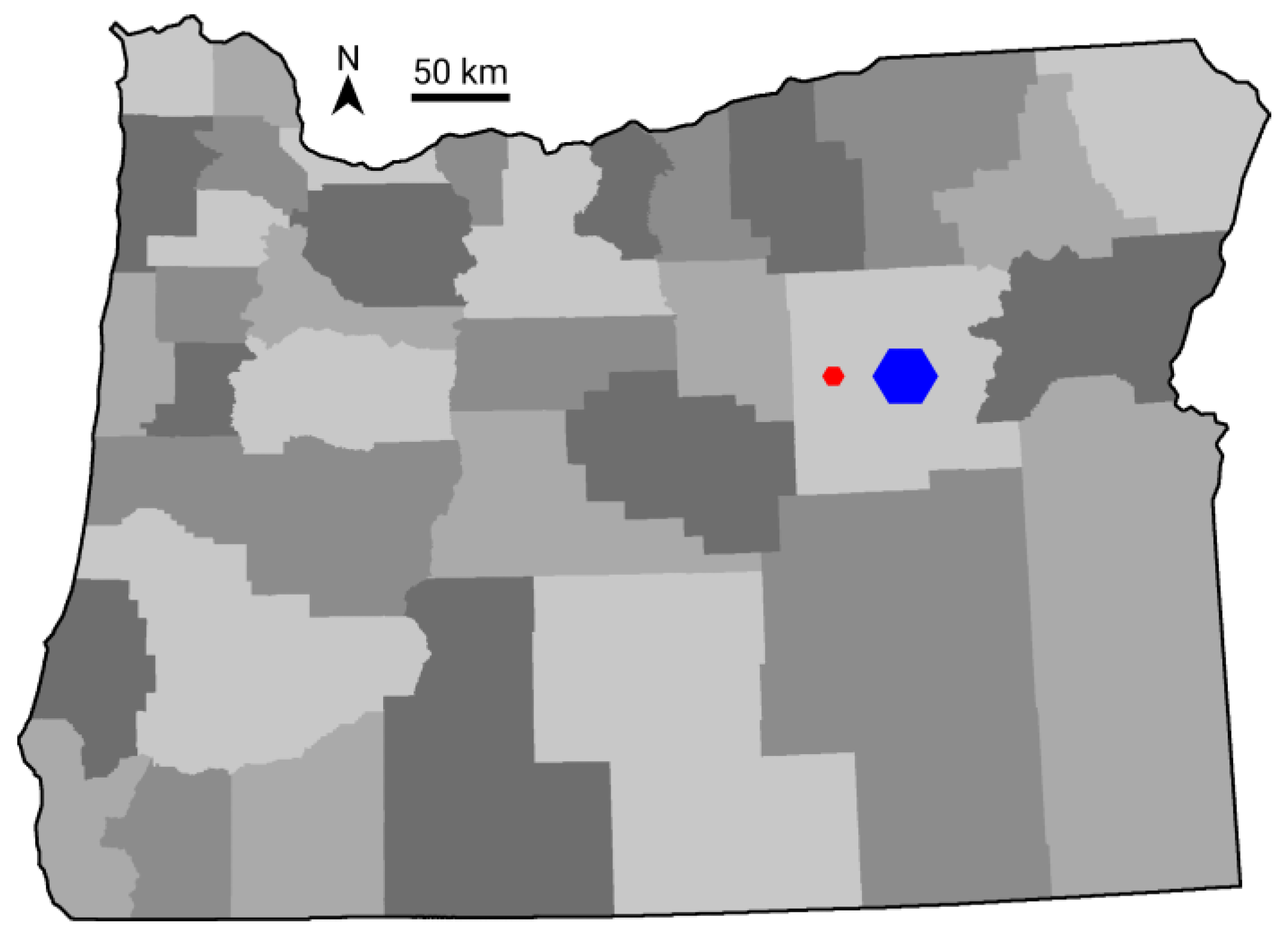
Figure 1. The state of Oregon, illustrating the locations of 36 counties (shades of gray) and the relative size of districts (red) and regions (blue).
Land 10 00438 g001
Figure 2. A schematic diagram of the spatial simulation model illustrating key mechanisms that run every day (except vaccination). All SIRD calculations are made at the block scale, and these values are aggregated to the larger spatial structures each day. Our three disease spread mechanisms are indicated in yellow.
Land 10 00438 g002
Figure 3. Numbers of new infections and deaths emerging from the spatial model incorporating social distancing (red and orange lines) and from Oregon COVID-19 records compiled by the New York Times (black and blue lines) [50]. COVID-19 testing in Oregon has been minimal throughout the pandemic, but was near zero when the disease began increasing within the state’s major metropolitan centers (A). The spread of COVID into rural parts of the state coincided with the 2020 holiday season, during which rates of viral transmission increased (B). Better adherence to human health guidelines in rural and suburban parts of Oregon contributed to a subsequent decline in cases (C).
Land 10 00438 g003
Figure 4. Daily infections resulting from five spatial vaccination strategies. Numbers of infections prior to vaccination are shown in black. These models all incorporate social distancing, and the results shown are mean values taken from 10 replicate simulations.
Land 10 00438 g004
Figure 5. Cumulative infections resulting from five spatial vaccination strategies, the non-spatial model with vaccination, and the spatial model without vaccination. Numbers of infections prior to vaccination are indicated by the solid black line. These models all incorporate social distancing, and the results shown are mean values taken from 10 replicate simulations.
Land 10 00438 g005
Figure 6. Spatial vaccination strategies emerging from one replicate each of the VPD, VPR, and VPC models. The number of individuals vaccinated is indicated by color, with lower numbers shown in blue, intermediate values in yellow, and the largest numbers in red.
Land 10 00438 g006
Table 1. Four spatial scales used in the HexSim COVID simulations.
ScaleQuantityMax Area
(Hexagons)
Max Area
(Hectares)
Block38,35537800
District30913978600
Region393336773,000
County36123,8092.7 M
Table 2. Data and parameters required by the simulation models.
Model InputDescriptionValue
Spatial DataPopulation SizeNumber per hexagon
Patch MapsBlocks
District
Regions
Counties
SIRD Ratesβ (infection)0.25
γ (recovery)0.064
δ (death)0.01
Spontaneous Infection RateDaily rate at which blocks are
seeded with a new infection,
converting one susceptible
individual into an infected.
1.0 × 10⁻⁷
Adjusted BetaThe model simulates social distancing
by replacing β with a smaller value we refer to as “adjusted β”.
CI is the lagged infections per 1000
individuals, computed by county.
SD, our social distancing coefficient, was set equal to 2.0.
β ( 1 C I S D )
VaccinationStatewide total3 million
Acquired immunity rate100%
Table 3. The spatial vaccination strategies and corresponding acronyms.
TitleVaccination StrategyDeployment Strategy
VURUnprioritizedRandom
VUUUniform
VPCPrioritizedCounty
VPRRegion
VPDDistrict
Publisher’s Note: MDPI stays neutral with regard to jurisdictional claims in published maps and institutional affiliations.