Article

Assessing the Impact of Urban Expansion on Surrounding Forested Landscape Connectivity across Space and Time

1
Institute of Digital Agriculture, Zhejiang Academy of Agricultural Sciences, Hangzhou 310021, China
2
School of Resource and Environmental Sciences, Wuhan University, Wuhan 430079, China
*
Author to whom correspondence should be addressed.
Land 2021, 10(4), 359; https://doi.org/10.3390/land10040359
Submission received: 27 January 2021 / Revised: 6 March 2021 / Accepted: 18 March 2021 / Published: 1 April 2021
(This article belongs to the Section Landscape Ecology)

Abstract

:
Landscape connectivity is important for all organisms as it directly affects population dynamics. Yet, rapid urbanization has caused serious landscape fragmentation, which is the primary contributor of species extinctions worldwide. Previous studies have mostly used spatial snap-shots to evaluate the impact of urban expansion on landscape connectivity. However, the interactions among habitats over time in dynamic landscapes have been largely ignored. Here, we demonstrated that overlooking temporal connectivity can lead to the overestimation of the impact of urban expansion. How much greater the overestimation is depends on the amount of net habitat loss. Moreover, we showed that landscape connectivity may have a delayed response to urban expansion. Our analysis shifts the way to understand the ecological consequences of urban expansion. Our framework can guide sustainable urban development and can be inspiring to conservation practices under other contexts (e.g., climate change).

1. Introduction

Worldwide, the population boom has resulted in rapid urban expansion [1] and dramatic land-use changes, which are considered as the primary drivers of landscape fragmentation and biodiversity loss [2,3]. An adequate degree of landscape connectivity plays a pivotal role in ecological processes such as colonization and extinction [4], ensuring resilience of metapopulations [5]. Understanding the impact of urban development on landscape connectivity and using suitable connectivity models to assess urban growth scenarios can, therefore, significantly contribute to balancing urban development and biodiversity conservation [6].
Certain relationships have been found between landscape connectivity and the rate [7,8], the form [9,10,11,12], and intensity [13,14] of urban growth. For example, dense urban development alleviates the encroachment to habitats but inevitably increases barrier effects of built-up areas [13]. Additionally, compact development maintains more connectivity than urban sprawl [15]. Yet, how different regional urban development strategies (uneven development vs. balanced development) affect landscape connectivity is rarely investigated.
Furthermore, only a handful of studies have provided impact assessments from a spatiotemporal perspective (e.g., refs. [16,17,18,19]), mainly due to that most of the connectivity models [20,21,22,23] are spatial snap-shots [24], which facilitate impact evaluation by comparing connectivity assessments performed independently at multiple time points. Nevertheless, these purely spatial connectivity models overlook the temporal interactions among habitat patches, such as the facilitation or impedance effect caused by the appearance or disappearance of stepping-stone habitat patches over time [17], so that they may generate misleading assessments (see schematic representation in Figure 1).
To bridge this gap, here we developed a framework that combines a cellular automata (CA) model with a recent spatiotemporal connectivity model [17]. We aimed to answer which regional urban development strategy is less detrimental to landscape connectivity, and investigate different behaviours of spatial-only connectivity and spatiotemporal connectivity under urban expansion. The CA model supports the design of the three urban development strategies (S1: uneven development that concentrates urban land in the mega-city; S2: balanced development; S3: controlling the mega-city size and put more urban land in other cities). The spatiotemporal connectivity model can capture the effects of temporal interactions of habitat patches. We selected the Three Gorges Reservoir Area (TGRA, SW China) as the study area for its high biological conservation values (one of the richest areas in terms of biodiversity in China; Wu, Huang [25]) and rapid urbanization [8].

2. Materials and Methods

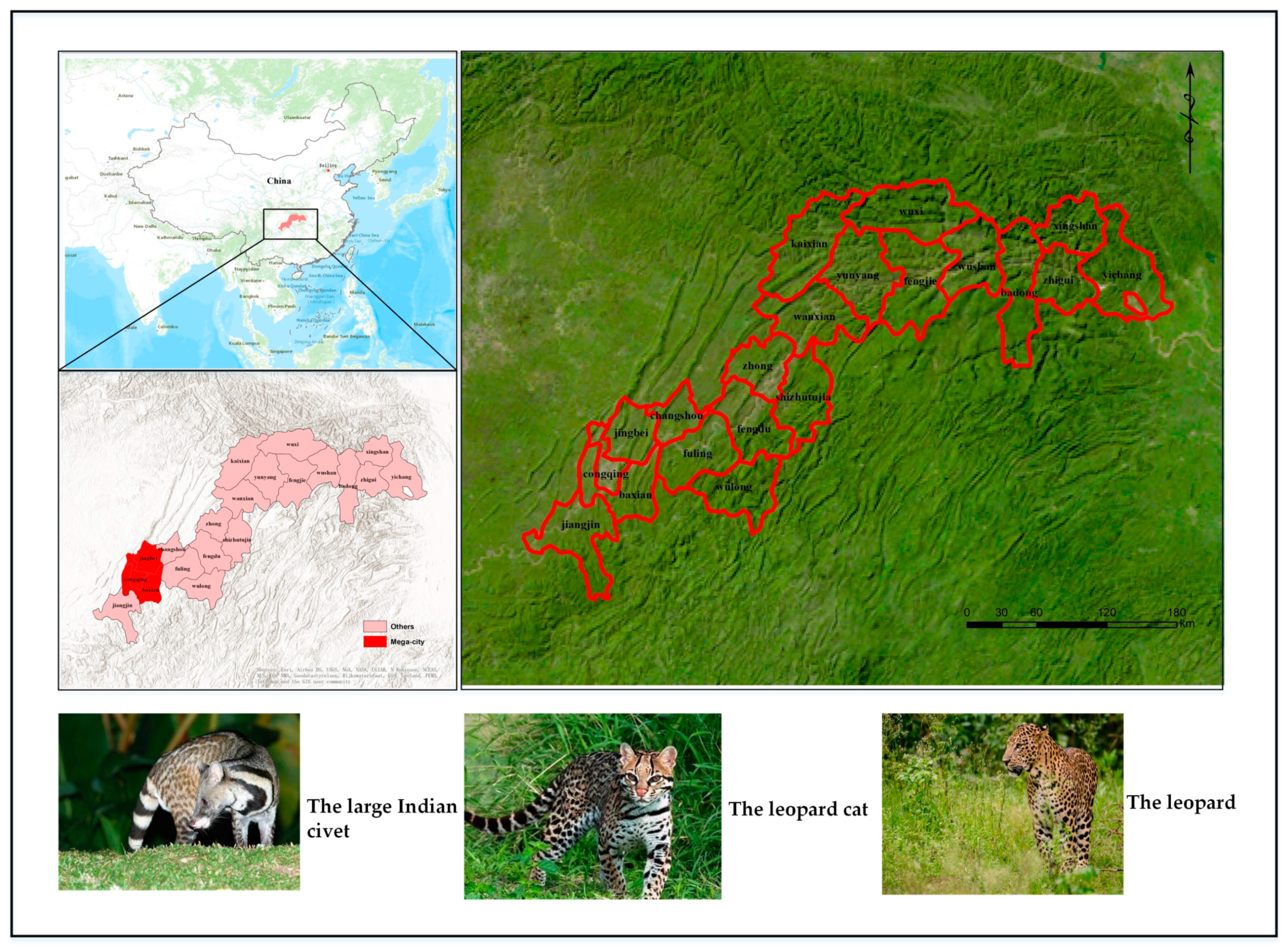
2.1. Study Area and Target Species

The TGRA is located in the middle catchment of the Yangtze River in China (Figure 2). It covers c. 58,000 km2 and includes multiple administrative districts of Chongqing City and Hubei Province. According to the national classification of urban size [26], there is one mega-city (i.e., Chongqing main city proper) in the TGRA. The TGRA is one of the richest areas in terms of biodiversity in China, and the biodiversity of genera and families is among the highest globally [25]. The TGRA has experienced fast urban expansion to resettle an enormous population of immigrants during the Three Gorges Dam Project, and the fast rate of urban expansion will continue as it is a key region in the Yangtze River Economic Belt [27]. Meanwhile, the Grain-to-Green Project (GTGP) has been implemented in this region to convert the cropland in the steep slope to the forested land since 2000, which significantly increase the forest area [28].
Three nationally protected animals inhabiting the TGRA: the large Indian civet (Viverra zibetha, represented by “LIC” hereafter), the leopard cat (Prionailurus bengalensis, “LC”) and the leopard (Panthera pardus, “L”) were selected as our target species, to represent a wide range of body sizes of local forest mammals. The home range sizes of the three species are 6 km2 [29], 12.7 km2 [30] and 28.2 km2 (the mean value of 5 collared individuals in Odden, Athreya [31]), respectively. As species natal dispersal distance is proportional to the home range size, the natal median dispersal distance of each target species was estimated as [32]:
Median   dispersal   distance   =   7 home   range   area
Therefore, natal median dispersal distances were estimated as: 14.7 km for the large Indian civet, 25.0 km for the leopard cat, and 37.2 km for the leopard. In addition, the data collected and used in this study are listed in Table 1.

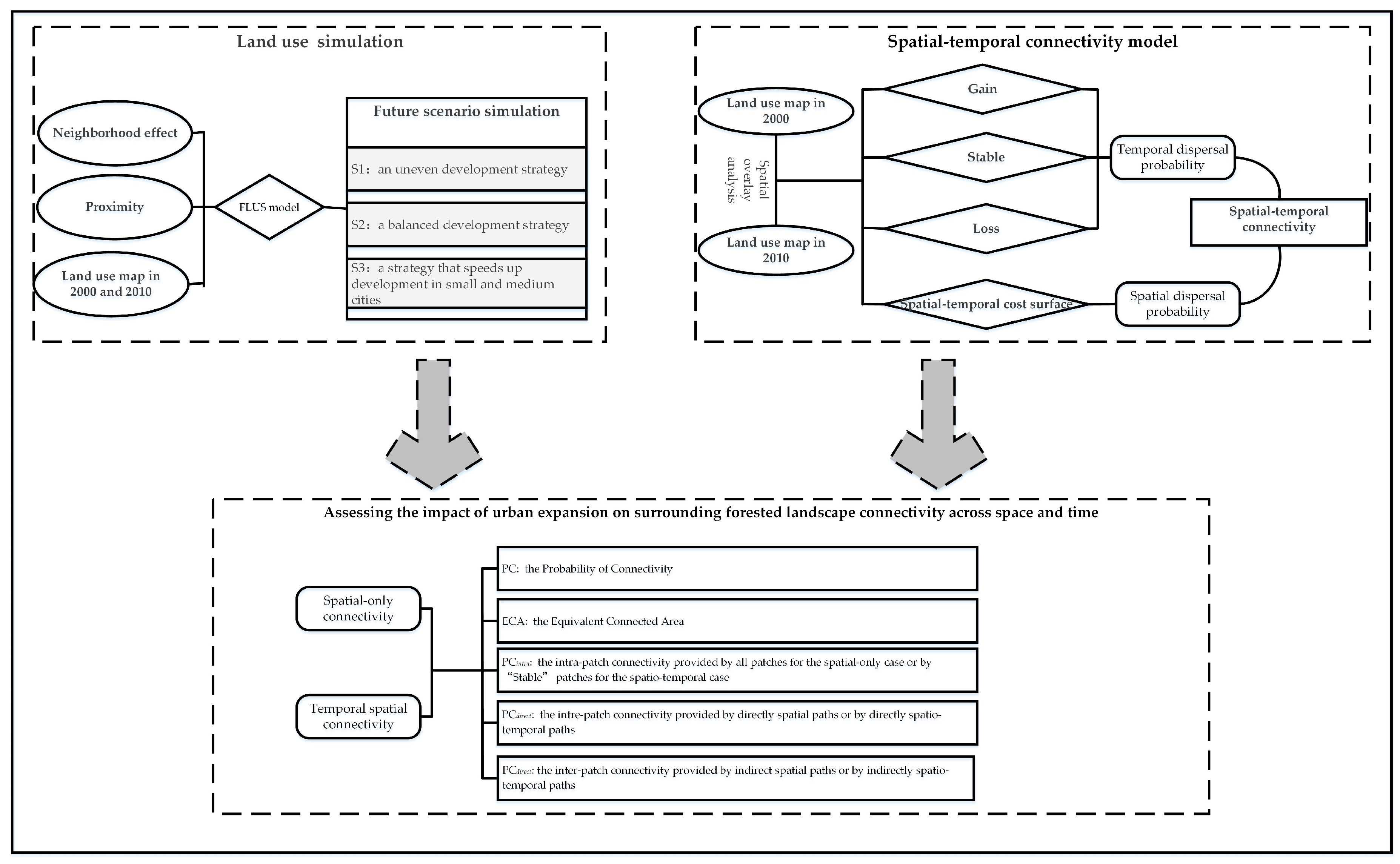
2.2. Research Framework

An overview of the research framework is displayed in Figure 3. Firstly, future urban expansion was simulated under three different development strategies by the FLUS model. Secondly, the connectivity model that fully takes account of spatiotemporal connections between patches was developed. Thirdly, we evaluated the effects of urban expansion on surrounding forest landscape connectivity based on connectivity metrics.

2.3. The Future Land Use Simulation Model

The Future Land Use Simulation (FLUS) model [35] is an artificial neuron network [36] (ANN) based CA model. We opted to use the FLUS model as it can better tackle the non-linear relationships in the land-use system than many other CA models [37,38]. First, the probability-of-occurrence of each land-use type on a grid cell is estimated through the ANN training based on a land-use map and other auxiliary geographical information, including terrain factors (elevation, slope and aspect), proximity factors (distance to the mega-city core, distance to common cities, distance to road, and distance to river), and socio-economic factors (GDP and population density). Second, the probability-of-occurrence is multiplied by the neighbourhood effect, inertia coefficient, and the conversion difficulty to obtain the total land-use conversion probability. This is to fully account for factors affecting landscape dynamics and efficiently implement spatial allocation, while also acknowledging that not all grid cells can be converted [39]. Third, based on the total probability, the roulette wheel selection method is applied to determine whether land-use conversion occurs on a grid cell or not. This is to reflect the competition within a land-use system. Please see Supplementary Materials Table S1 or Liu, Liang [35] for detailed information.

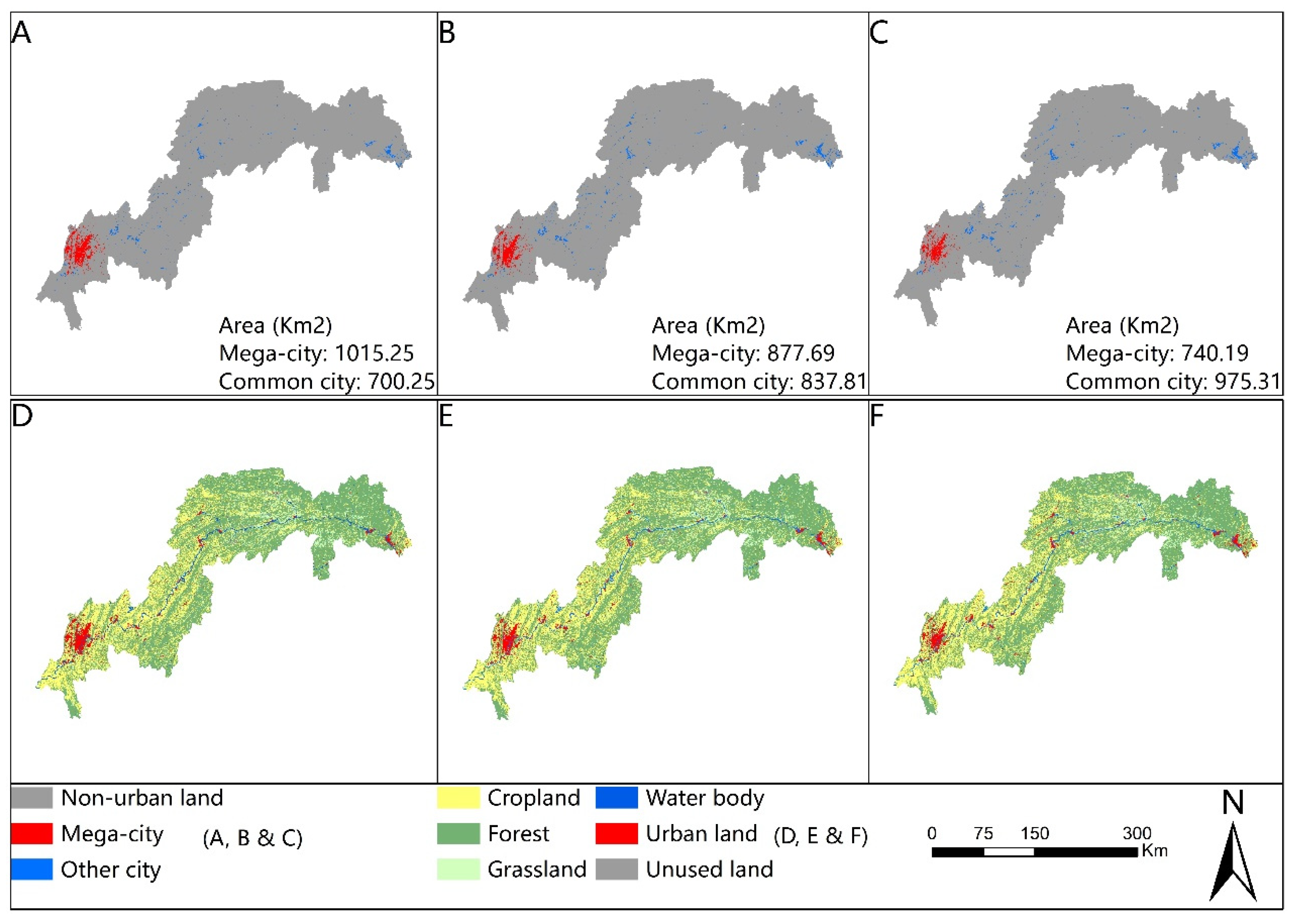
2.4. Simulating Different Regional Urban Development Strategies

All grid cells were classified into “mega-city urban land”, “common city urban land” and “non-urban land”, based on the administrative districts which they are located in and the land-use type which the grid cell belongs to. As population growth necessitates the development of urban land [40], we calculated future urban land demands according to the predicted population growth. We assumed that the increase rate of population declines with the increase in population amount, and thus the logistic model was used (see Supplementary Materials Table S1). Based on the predicted urban land demand, we designed three urban development strategies (S1–S3). S1 is an uneven development strategy that concentrates 75% of the new urban land in the mega-city. S2 is a balanced development strategy that equally places the new urban land in the mega-city and the other cities. S3 is a strategy that speeds up development in small and medium cities (by allocating 75% of the new urban land) while controls urban expansion in the mega-city.
The potential urban expansion under different strategies were simulated by the FLUS model, and were then overlaid on the current land-use map (with six land-use types) to create future land-use maps. This was to ensure that no transitions would occur among other non-urban land-use types, so that the connectivity change is only dependent on urban expansion (i.e., habitat loss and stronger barrier effect caused by conversion from non-urban land to urban land).

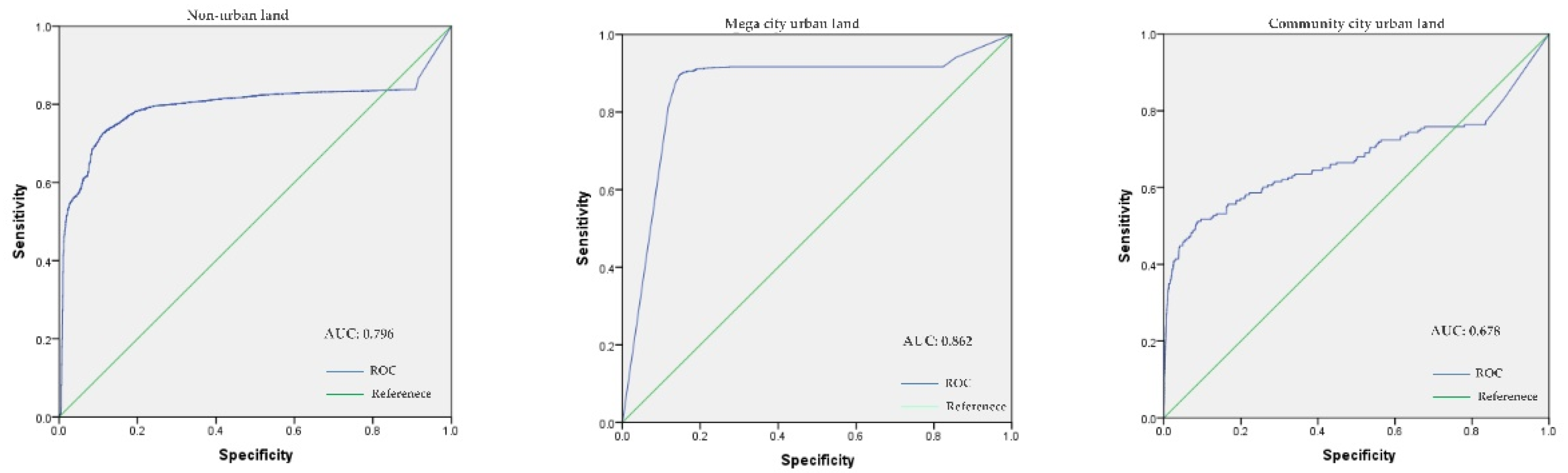
2.5. Model Validation

The FLUS model was validated through two aspects: (1) the Area under a Receiver Operating Characteristic curve (AUC) values [41] were applied to quantify the ANN performance in fitting the probability-of-occurrence of the individual land-use type (Figure 4), and (2) the fuzzy Kappa index [42] was used to evaluate the goodness-of-fit of simulation landscape in 2010. For the first aspect, a perfectly fitted result yields an AUC value of 1 while a completely random model yields an AUC value of 0.5. The AUC values of the three land-use types are 0.796, 0.862, and 0.678, respectively, indicating that the fitted probability-of-occurrence of the three land-uses can be well explained by the selected driving forces. For the second aspect, the fuzzy kappa indices of the three land-use types are 0.84, 0.88, and 0.82 respectively; and the overall fuzzy Kappa is 0.85, indicating a considerable high goodness-of-fit of the simulation result. The receiver operating characteristic curve (ROC) curves were obtained through SPSS 23, and the fuzzy Kappa was obtained through Map Comparison Kit [43].

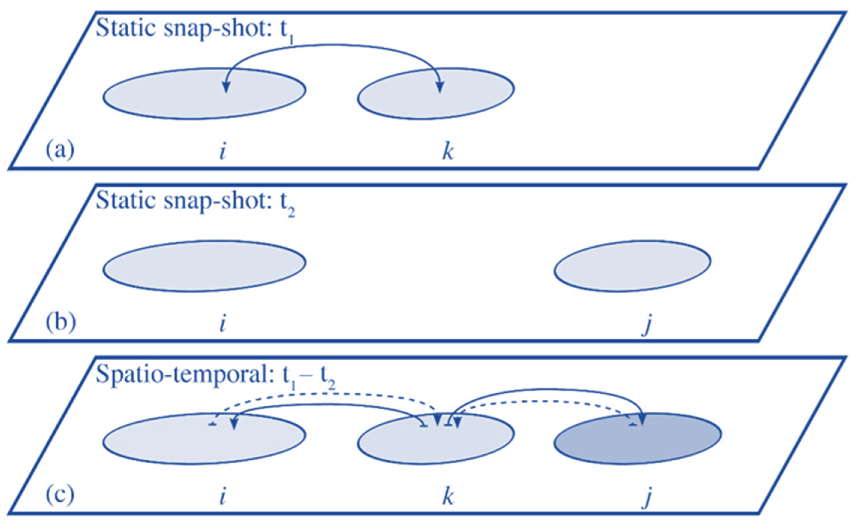
2.6. Spatial-Temporal Connectivity Model

Conceptually, a spatiotemporal path across a habitat network represents the possibility of an individual moving from a given habitat patch (i.e., node in spatial graph terminology) at time t 1 to another patch at t 2 ( t 1 < t 2 ). For conservation applications, such a path also indicates the likelihood that an individual will persist from t 1 to t 2 in a changing landscape [17].
We deemed the forest patch whose (1) size is larger than the home range size of a given species and (2) location is 200 m away from urban land and roads as the habitat node of the corresponding species [17]. This selection was to ensure the species’ relatively long-term persistence and adequate tolerance to anthropogenic activities. However, tolerance to anthropogenic activities (i.e., distance to construction land) was considered invariable among the three focal species given that we did not find documents reporting such information. Nodes were attributed to the corresponding patch sizes.
Given two time points ( t 1 , t 2 ), all habitat patches in a landscape can be classified into three types by overlay analysis for habitat maps in t 1 and t 2 , including (1) Gain: not habitat in t 1 but habitat in t 2 , (2) Stable: habitat in both t 1 and t 2 , and (3) Loss: habitat in t 1 but not habitat in t 2 . To persist in a dynamic landscape, an individual must stay in a Stable habitat patch, or disperse from a habitat patch at t 1 (i.e., Loss or Stable) to another habitat patch at t 2 (i.e., Gain or Stable).
Temporal interactions between patches can occur if and only if they simultaneously exist in the landscape for a while, that is, having temporal overlap. For example, a Loss patch and a Stable patch must have temporal overlap, since that Loss patch can only lose habitat after an intermediate time point t x ( t 1 < t x < t 2 ) and Stable patch persists in the landscape through t 1 to t 2 . Similarly, a Gain patch and a Stable patch can also have temporal interactions. In cases where temporal overlap exists, the probability of temporal interactions between these two patches is assigned as 1 (i.e., p i j t = 1 ). However, for a Loss patch and a Gain patch, they may or may not have temporal interactions since we do not know at time point the Loss patch loses habitat and the Gain patch gains habitat. Therefore, in this case, the probability of temporal interactions is assigned as 0.5 (i.e., p i j t = 0.5 ).
Additionally, the temporal links can also be classified into two types: (1) the essential link and (2) the auxiliary link [17]. An essential link is a link that, alone, is enough to ensure that an individual can move from habitat node at t 1 to another habitat node at t 2 . An auxiliary link is a link that cannot achieve the transportation for individuals as an essential link does. However, through a path that combines consecutive auxiliary links (and at least one essential link), an individual may be able to indirectly move from a habitat node at t 1 to another habitat node at t 2 . By doing so, more habitats are reachable than by using essential links only. For example, for a path “Loss -> Loss -> Stable”, the first link is an auxiliary link because when dispersing from Loss to Loss, no habitat is available for that individual to ensure persistence. The second link is an essential link because two endpoints have habitat at the beginning and at the end, such that it alone can ensure that individual’s persistence. Thus, a successful temporal path can either be (1) a direct path that consists of a single essential link or (2) an indirect path constituting of any combinations of auxiliary links and essential links, as long as at least there is one essential link. The probability of each movement scenario is listed in Table 2.
For the spatial links, the movement probability from node i to node j (represented as p i j s ) is determined by using an exponential function of the species dispersal capabilities and the distances between patches [17]: p i j s = e k d i j ; where k is a species-specific constant reflecting the dispersal ability, and d i j is the distance between i and j . Here, the distance between patches is the cost-weighted distance derived from the least-cost modelling [17], to consider the spatial heterogeneity of impedance of the landscape (see Supplementary Table S2 for the cost of each land-use type). Some studies noticed that the landscape impedance may vary with time [44,45], hence such variations were also taken into account. Given that detailed information about when land-use changes occur during t 1 and t 2 is unavailable, we obtained the spatiotemporal cost surface by taking the average between the cost surfaces in t 1 and t 2 . For instance, for a grid cell p belonging to the cropland at t 1 and being converted to the grassland in t 2 , its cost value in the spatiotemporal cost surface is the average between cost values of the cropland and the grassland. The median dispersal distance was multiplied by the median cost value of the dynamic cost surface from 2000 to 2010, and the result determined the dispersal threshold corresponding to a spatial dispersal probability of 0.5 (i.e., to parameterise k ; Gurrutxaga, Rubio [46]).
The ultimately spatiotemporal links and their dispersal probabilities ( p i j s t ) are obtained through multiplying the temporal dispersal probability ( p i j t ) by the spatial dispersal probability ( p i j s ), which is formulated as:
p i j s t = p i j t × p i j s
By doing so, the connectivity model fully takes account of all possibilities of spatiotemporal connections between patches, in either direct or indirect fashion, while also acknowledging that not all paths will lead to a successful transportation for an individual. The overlay analysis was implemented in ArcGIS 10.2, the least-cost modelling was implemented in Linkage Mapper V1.1 [47].

2.7. Connectivity Metrics

Network theory is a powerful approach to measure connectivity [48], and five network-based metrics: the Probability of Connectivity ( P C ; Saura and Pascual-Hortal [23]), the Equivalent Connected Area ( E C A ; Saura, Estreguil [49]), and the three P C s fractions [50] are popular connectivity metrics for conservation planning. These metrics were adapted to spatiotemporal connectivity model by replacing the spatial-only dispersal probability p i j s in the original formulas with the spatiotemporal dispersal probability p i j s t (with the subscript “st”). P C is defined as the probability that two individuals randomly placed within a landscape fall into habitat patches that are reachable for each other across the habitat network [23], and is formulated as:
P C = i = 1 n j = 1 n a i a j p i j * A l 2
where a i and a j denote the area of patch i and j , respectively; A l is the area of the study site; p i j * is the maximum product probability of all possibly spatial paths ( p i j s ) for the spatial-only connectivity case (original P C ), or of all possibly spatiotemporal paths ( p i j s t ) for the spatiotemporal connectivity case ( P C s t ).
E C A and E C A s t indicate the amount of spatially reachable habitat and the amount of spatiotemporally reachable habitat, and are formulated as the square root of the numerator of P C and P C s t , respectively.
Moreover, P C ’s fractions are formulated as Equations (4)–(6):
P C i n t r a = i = 1 n a i 2 A l 2
P C d i r e c t = i = 1 n j = 1 ,   i j n a i a j p i j A l 2
P C s t e p = i = 1 n j = 1 ,   i j n a i a j ( p i j * p i j ) A l 2
where P C i n t r a corresponds to the intra-patch connectivity [51] provided by all patches for the spatial-only case or by “Stable” patches for the spatiotemporal case ( P C i n t r a ,   s t ); P C d i r e c t corresponds to the inter-patch connectivity provided by directly spatial paths (for the spatial-only case) or by directly spatiotemporal paths (for the spatiotemporal case, P C d i r e c t ,   s t ) without using stepping-stones; P C s t e p corresponds to the inter-patch connectivity provided by indirect spatial paths (for the spatial-only case) or by indirectly spatiotemporal paths (for the spatiotemporal case, P C s t e p ,   s t ) that pass through intermediate stepping-stones. We also built a linear univariate model to present the relationship between the amount of habitat change and the contribution of E C A s t compared with E C A at t 2 .

3. Results

3.1. Urban Expansion and Habitat Change in Different Urban Development Scenarios

Under S1–S3 at 2020, the urban size is predicted to be 1716 km2, which is over twice the size in 2000. The mega-city takes up 59.2% of the total urban land in S1 while only 43.1% in S3. New urban land is put to west and east Chongqing main city proper in S1, while put to cities in northeast TGRA that are close to large and continuous tracts of forests in S2 and S3 (Figure 5). From 2000 to 2010, the three focal species gained more habitats and LIC had the largest habitat increment (+2.99%), but they suffer habitat loss in S1–S3 at 2020. Among all scenarios in 2020, S3 has the severest habitat shrinkage for all considered species while slight habitat loss occurs in S1. Among all target species, L’s habitats are more affected by urban expansion (Table 3).

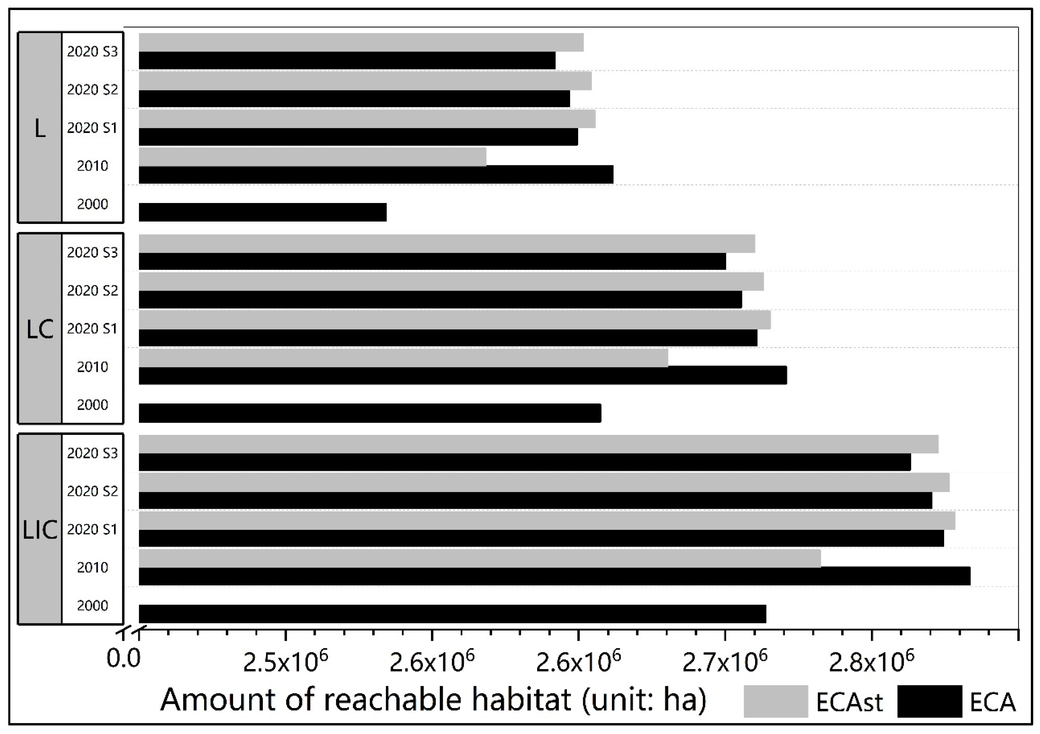
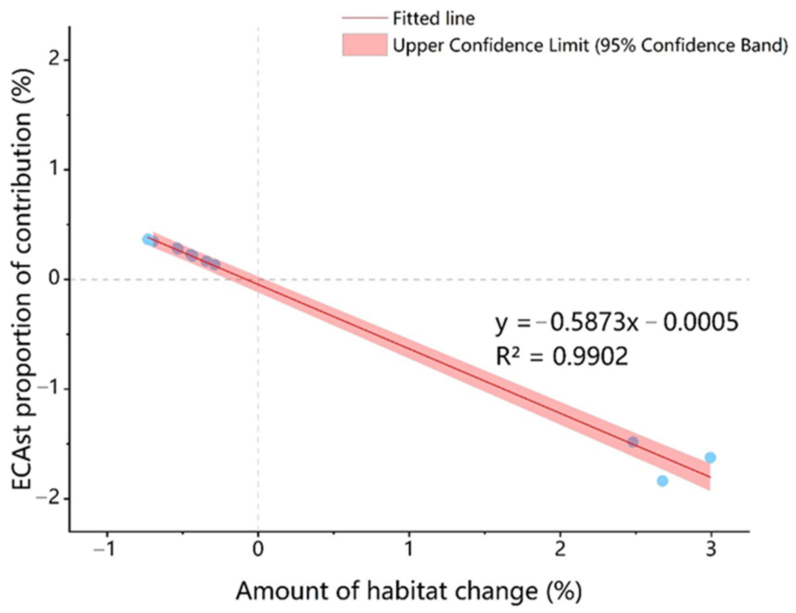
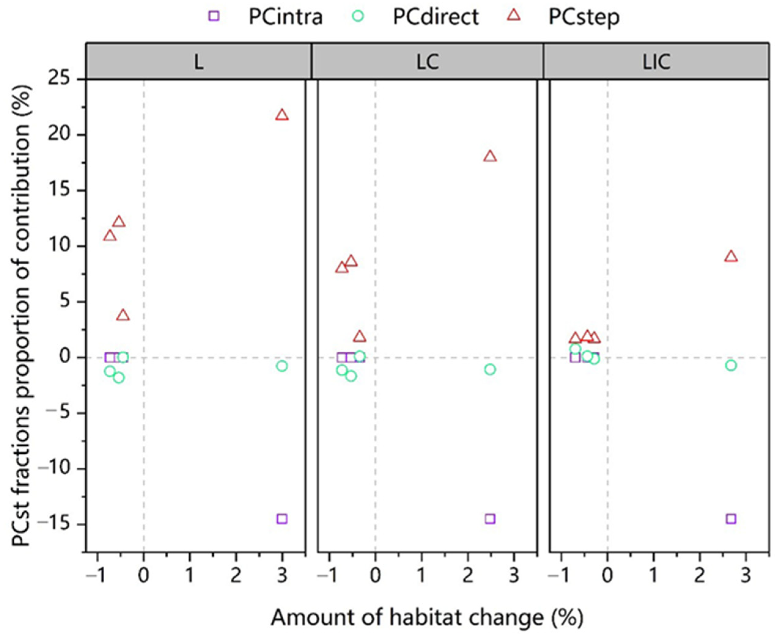
3.2. The Spatial-Only and Spatiotemporal Connectivity in Different Scenarios

During 2000 and 2010, the amount of spatiotemporally reachable habitat (indicated by E C A s t , see Methods) is smaller than the amount of spatial-only reachable habitat ( E C A ) in 2010 for all target species (Figure 6). However, from 2010 to 2020, E C A s t exceeds E C A in 2020 and this holds for any species under any scenario. The linear model suggests that, when the amount of habitat increases or decreases by 1%, E C A s t will be c. 0.5% lower or higher than E C A at t 2 (Figure 7). Additionally, for each species, E C A increases during 2000 and 2010 due to habitat expansion and decreases during 2010 and 2020 due to habitat shrinkage, while E C A s t is higher in the period from 2010 to 2020 than in the period from 2000 to 2010.
For contribution of P C s t fractions, when habitat area increases by c. 3% (corresponding to the habitat increment during 2000 and 2010), P C i n t r a s t is c. 15% lower than P C i n t r a for all focal species, whereas P C s t e p s t has relatively large contribution than P C s t e p (Figure 8), which ranges from 9% (for LIC) to 22% (for L). Under S1–S3, P C i n t r a s t and P C i n t r a have no difference and P C d i r e c t s t is slightly lower than P C d i r e c t , while remarkable contributions were found in P C s t e p s t for LC and L in scenarios with more dramatic habitat losses (i.e., in S2 and S3).

4. Discussion

The simulation results and consequential connectivity changes demonstrate that regional urban development strategies have direct impacts on landscape fragmentation. In the TGRA, the strategy that concentrates new urban land in the mega-city helps to maintain more connectivity for all target species than other strategies. Natural habitats near the mega-city are much fewer than those near the other cities, so that concentrating urban land in the mega-city reduces the encroachment to habitats. This finding agrees with the Urban-rural Master Planning of Chongqing City, which articulates that the dominant function of the northeast TGRA is biodiversity conservation, rather than urban development.
The impact also varies by species with different dispersal capabilities (Figure 5). Urban expansion seems to have larger negative effects to species with long dispersal capacity, which is contrary to findings in previous studies suggesting that such impact declined with the rise in dispersal capacity [52,53]. However, the previous studies did not account for whether a patch could be viewed as a habitat for a given species or not (i.e., the patch size should be larger than the species home range size), hence the trade-off between the intra-patch and the inter-patch connectivity (i.e., lower intra-patch connectivity provided by fewer habitats vs. higher inter-patch connectivity provided by stronger dispersal ability) was ignored. In our analysed landscape, the higher connectivity decline of long dispersers mainly results from the habitat loss, rather than from the barrier effect and the loss of stepping-stones habitat patches.
Spatiotemporal connectivity and spatial-only connectivity have significantly different responses to urban expansion and the resulting land-use change. Spatial-only connectivity has an immediate rise or fall when habitats are gained or lost (e.g., at 2010 & the three scenarios at 2020). However, the spatiotemporal connectivity may still increase (e.g., E C A s t in the period from 2010 to 2020; Figure 5) despite the habitat shrinkage in the period (Table 3). This can be explained by the delayed biodiversity responses to land-use change, which are commonly studied in extinction debt research [54,55]. Landscape connectivity is recognised to play a crucial role in affecting relaxation times (i.e., time lags) and their trajectories [56]. By incorporating temporal connections that do not exist from the perspective of the purely spatial connectivity, habitats are linked in a spatiotemporal fashion. Such dynamics are essential to acknowledge the contribution of connectivity to relaxation times and to capture the lag effect, which cannot be embodied in purely spatial connectivity models. Additionally, in a rapidly changing landscape, more spatiotemporal connected habitat mosaics may be created [17], which can enhance rescue effects [57] or restore local extinctions with recolonizations [55]. Hence, we demonstrated that, the connectivity decline and the risk of species extinction due to urban expansion may be overestimated by previous studies using temporally static connectivity models. The spatiotemporal connectivity can better reflect the lag effect, can exert influences on duration and trajectory of relaxation time, and can help to prevent local and/or global species extinctions through the contribution of temporal connectivity, especially in landscapes where dramatic habitat loss occurs, such as those experiencing rapid urbanization ones.
The significance of the spatiotemporal connectivity is directly affected by the net habitat amount change. We found that the spatiotemporal connectivity exceeds the spatial-only connectivity for the net habitat loss cases, whereas the opposite is true for the net habitat gain cases. This finding agrees with Martensen, Saura [17]. The relationship could be described by a linear model, in which every 1% of net habitat loss or gain could result in nearly 0.5% of spatiotemporal connectivity positive or negative contribution compared with spatial-only connectivity. We further investigated why the spatiotemporal connectivity ends up having no additional contribution when additional habitats are gained, and found that the reason lies in the difference between the spatiotemporally and the spatially intra-patch connectivity. The intra-patch connectivity for the spatiotemporal case is only provided “Stable” patches (see Methods), while for the spatial-only case, it is provided by all patches in the end of term, which include both “Stable” and “Gain” patches in the net habitat gain landscapes. Therefore, the latter case can provide more intra-patch connectivity and further lead to a higher estimated connectivity.
Moreover, we noticed that the spatiotemporal connectivity mainly contributes to improving connectivity through the stepping-stone effect ( P C s t e p s t , see Figure 8). This shows that most of spatiotemporal connections occur through habitats that are gained or lost in temporal steps and are used as stepping-stones in temporal paths [58]. This also explains why the spatiotemporal connectivity has higher contribution for long dispersers than for short dispersers, as long dispersers experience more dramatic habitat change in our case, so that the increasing stepping-stone effect over time boosts a higher overall spatiotemporal connectivity.
The spatiotemporal connectivity model should have broad applications in any dynamic landscape, while it also has some limitations. Future research that investigates how to incorporate other species traits, such as longevity, into the current spatiotemporal model will be desired. For example, a long-lived species may better take advantage of spatiotemporal links across the habitat network than another short-lived species, as the former have a longer temporal overlap with patch persistence in its lifespan than the latter.

5. Conclusions

To conclude, our results demonstrated that previous studies had overestimated the impact of urban expansion to landscape connectivity. The analysis also highlighted the need to shift from the spatial-only perspective to the spatiotemporal perspective, as it helps to incorporate the delayed biodiversity response to land-use change in practical urban planning. The spatiotemporal connectivity should find its place in many future sustainable studies, such as biodiversity conservation in diverse climate scenarios.

Supplementary Materials

The following are available online at https://www.mdpi.com/article/10.3390/land10040359/s1. Table S1: The terminology, the formula and the description in the FLUE model, Table S2: Movement cost characterizing the impedance effect of each land-use type.

Author Contributions

Conceptualization, Z.R. and J.H.; methodology, Z.R.; validation, Q.Y. and J.H.; formal analysis, Z.R. and Q.Y.; investigation, Q.Y.; resources, Z.R.; data curation, Q.Y.; writing—original draft preparation, Z.R.; writing—review and editing, Q.Y. and J.H.; visualization, Z.R.; supervision, J.H.; project administration, Z.R. and J.H.; funding acquisition, Z.R. and J.H. All authors have read and agreed to the published version of the manuscript.

Funding

This research was funded by the National Natural Science Foundation of China, grant number 41871301.

Institutional Review Board Statement

Not applicable.

Informed Consent Statement

Not applicable.

Data Availability Statement

The data will be made available should the manuscript is accepted.

Acknowledgments

We would like to thank Junlong Huang for helpful comments on the earlier version of this manuscript.

Conflicts of Interest

The authors declare no conflict of interest.

References

  1. Seto, K.C.; Guneralp, B.; Hutyra, L.R. Global forecasts of urban expansion to 2030 and direct impacts on biodiversity and carbon pools. Proc. Natl. Acad. Sci. USA 2012, 109, 16083–16088. [Google Scholar] [CrossRef] [PubMed] [Green Version]
  2. Sala, O.E.; Chapin, F.S., 3rd; Armesto, J.J.; Berlow, E.; Bloomfield, J.; Dirzo, R.; Huber-Sanwald, E.; Huenneke, L.F.; Jackson, R.B.; Kinzig, A.; et al. Global biodiversity scenarios for the year 2100. Science 2000, 287, 1770–1774. [Google Scholar] [CrossRef]
  3. McKinney, M.L. Urbanization as a major cause of biotic homogenization. Biol. Conserv. 2006, 127, 247–260. [Google Scholar] [CrossRef]
  4. Bauer, S.; Hoye, B.J. Migratory animals couple biodiversity and ecosystem functioning worldwide. Science 2014, 344, 1242552. [Google Scholar] [CrossRef]
  5. Allen, C.R.; Angeler, D.G.; Cumming, G.S.; Folke, C.; Twidwell, D.; Uden, D.R. Quantifying spatial resilience. J. Appl. Ecol. 2016, 53, 625–635. [Google Scholar] [CrossRef]
  6. Perkl, R.; Norman, L.M.; Mitchell, D.; Feller, M.; Smith, G.; Wilson, N.R. Urban growth and landscape connectivity threats assessment at Saguaro National Park, Arizona, USA. J. Land Use Sci. 2018. [Google Scholar] [CrossRef]
  7. Troupin, D.; Carmel, Y. Landscape patterns of development under two alternative scenarios: Implications for conservation. Land Use Policy 2016, 54, 221–234. [Google Scholar] [CrossRef]
  8. Huang, Y.; Huang, J.-L.; Liao, T.-J.; Liang, X.; Tian, H. Simulating urban expansion and its impact on functional connectivity in the Three Gorges Reservoir Area. Sci. Total Environ. 2018, 643, 1553–1561. [Google Scholar] [CrossRef]
  9. Bierwagen, B.G. Connectivity in urbanizing landscapes: The importance of habitat configuration, urban area size, and dispersal. Urban. Ecosyst. 2006, 10, 29–42. [Google Scholar] [CrossRef]
  10. Mitsova, D.; Shuster, W.; Wang, X.H. A cellular automata model of land cover change to integrate urban growth with open space conservation. Landsc. Urban. Plann. 2011, 99, 141–153. [Google Scholar] [CrossRef]
  11. Grafius, D.R.; Corstanje, R.; Siriwardena, G.M.; Plummer, K.E.; Harris, J.A. A bird’s eye view: Using circuit theory to study urban landscape connectivity for birds. Landsc. Ecol. 2017, 32, 1771–1787. [Google Scholar] [CrossRef]
  12. Huang, J.L.; He, J.H.; Liu, D.F.; Li, C.; Qian, J. An ex-post evaluation approach to assess the impacts of accomplished urban structure shift on landscape connectivity. Sci. Total Environ. 2018, 622, 1143–1152. [Google Scholar] [CrossRef]
  13. Aguilera, F.; Valenzuela, L.M.; Botequilha-Leitao, A. Landscape metrics in the analysis of urban land use patterns: A case study in a Spanish metropolitan area. Landsc. Urban. Plann. 2011, 99, 226–238. [Google Scholar] [CrossRef]
  14. Marulli, J.; Mallarach, J.M. A GIS methodology for assessing ecological connectivity: Application to the Barcelona Metropolitan Area. Landsc. Urban. Plann. 2005, 71, 243–262. [Google Scholar] [CrossRef]
  15. Tannier, C.; Bourgeois, M.; Houot, H.; Foltete, J.C. Impact of urban developments on the functional connectivity of forested habitats: A joint contribution of advanced urban models and landscape graphs. Land Use Policy 2016, 52, 76–91. [Google Scholar] [CrossRef]
  16. Huang, J.L.; Andrello, M.; Martensen, A.C.; Saura, S.; Liu, D.F.; He, J.H.; Fortin, M.J. Importance of spatio–temporal connectivity to maintain species experiencing range shifts. Ecography 2020, 43, 591–603. [Google Scholar] [CrossRef]
  17. Martensen, A.C.; Saura, S.; Fortin, M.-J. Spatio-temporal connectivity: Assessing the amount of reachable habitat in dynamic landscapes. Methods Ecol. Evol. 2017, 8, 1253–1264. [Google Scholar] [CrossRef]
  18. Saura, S.; Bodin, Ö.; Fortin, M.-J. Stepping stones are crucial for species’ long-distance dispersal and range expansion through habitat networks. J. Appl Ecol. 2014, 51, 171–182. [Google Scholar] [CrossRef]
  19. Watts, A.; Schlichting, P.; Billerman, S.; Jesmer, B.; Micheletti, S.; Fortin, M.-J.; Funk, C.; Hapeman, P.; Muths, E.; Murphy, M. How spatio-temporal habitat connectivity affects amphibian genetic structure. Front. Genet. 2015, 6. [Google Scholar] [CrossRef] [Green Version]
  20. Hanski, I.; Ovaskainen, O. The metapopulation capacity of a fragmented landscape. Nature 2000, 404, 755–758. [Google Scholar] [CrossRef]
  21. Moilanen, A.; Nieminen, M. Simple Connectivity Measures in Spatial Ecology. Ecology 2002, 83, 1131–1145. [Google Scholar] [CrossRef]
  22. Pascual-Hortal, L.; Saura, S. Comparison and development of new graph-based landscape connectivity indices: Towards the priorization of habitat patches and corridors for conservation. Landsc. Ecol. 2006, 21, 959–967. [Google Scholar] [CrossRef]
  23. Saura, S.; Pascual-Hortal, L. A new habitat availability index to integrate connectivity in landscape conservation planning: Comparison with existing indices and application to a case study. Landsc. Urban. Plann. 2007, 83, 91–103. [Google Scholar] [CrossRef]
  24. Mui, A.B.; Caverhill, B.; Johnson, B.; Fortin, M.J.; He, Y.H. Using multiple metrics to estimate seasonal landscape connectivity for Blanding’s turtles (Emydoidea blandingii) in a fragmented landscape. Landsc. Ecol. 2017, 32, 531–546. [Google Scholar] [CrossRef]
  25. Wu, J.G.; Huang, J.H.; Han, X.G.; Xie, Z.Q.; Gao, X.M. Three-Gorges Dam—Experiment in habitat fragmentation? Science 2003, 300, 1239–1240. [Google Scholar] [CrossRef] [PubMed]
  26. The State Council of the People’s Republic of China. The Notification on Adjusting the Classification Standard of Urban Size; The State Council of the People’s Republic of China: Beijing, China, 2014.
  27. Xu, X.; Yang, G.; Tan, Y.; Liu, J.; Hu, H. Ecosystem services trade-offs and determinants in China’s Yangtze River Economic Belt from 2000 to 2015. Sci. Total Environ. 2018, 634, 1601–1614. [Google Scholar] [CrossRef] [PubMed]
  28. Hua, F.; Wang, X.; Zheng, X.; Fisher, B.; Wang, L.; Zhu, J.; Tang, Y.; Yu, D.W.; Wilcove, D.S. Opportunities for biodiversity gains under the world’s largest reforestation programme. Nat. Commun. 2016, 7, 12717. [Google Scholar] [CrossRef] [Green Version]
  29. Rabinowitz, A.R. Behavior and movements of sympatric civet species in HUAI-KHA-KHAENG Wildlife Sanctuary, Thailand. J. Zool. 1991, 223, 281–298. [Google Scholar] [CrossRef]
  30. Grassman, L.I.; Tewes, M.E.; Silvy, N.J.; Kreetiyutanont, K. Spatial organization and diet of the leopard cat (Prionailurus bengalensis) in north-central Thailand. J. Zool. 2005, 266, 45–54. [Google Scholar] [CrossRef]
  31. Odden, M.; Athreya, V.; Rattan, S.; Linnell, J.D.C. Adaptable Neighbours: Movement Patterns of GPS-Collared Leopards in Human Dominated Landscapes in India. PLoS ONE 2014, 9. [Google Scholar] [CrossRef] [Green Version]
  32. Bowman, J.; Jaeger, J.A.G.; Fahrig, L. Dispersal distance of mammals is proportional to home range size. Ecology 2002, 83, 2049–2055. [Google Scholar] [CrossRef]
  33. Jarvis, A.; Reuter, H.I.; Nelson, A.; Guevara, E. Hole-filled Seamless SRTM Data V4. International Centre for Tropical Agriculture (CIAT). Available online: http://srtm.csi.cgiar.org (accessed on 19 December 2020).
  34. Center for International Earth Science Information Network—CIESIN—Columbia University; Information Technology Outreach Services—ITOS—University of Georgia. Global Roads Open Access Data Set, Version 1 (gROADSv1); NASA Socioeconomic Data and Applications Center (SEDAC): Palisades, NY, USA, 2013. [Google Scholar]
  35. Liu, X.P.; Liang, X.; Li, X.; Xu, X.C.; Ou, J.P.; Chen, Y.M.; Li, S.Y.; Wang, S.J.; Pei, F.S. A future land use simulation model (FLUS) for simulating multiple land use scenarios by coupling human and natural effects. Landsc. Urban. Plan. 2017, 168, 94–116. [Google Scholar] [CrossRef]
  36. Openshaw, S.; Openshaw, C. Artificial Intelligence in Geography; John Wiley & Sons: Chichester, UK, 1997. [Google Scholar]
  37. Lin, Y.P.; Chu, H.J.; Wu, C.F.; Verburg, P.H. Predictive ability of logistic regression, auto-logistic regression and neural network models in empirical land-use change modeling—A case study. Int. J. Geogr. Inf. Sci. 2011, 25, 65–87. [Google Scholar] [CrossRef] [Green Version]
  38. Li, X.; Chen, G.; Liu, X.; Liang, X.; Wang, S.; Chen, Y.; Pei, F.; Xu, X. A New Global Land-Use and Land-Cover Change Product at a 1-km Resolution for 2010 to 2100 Based on Human–Environment Interactions. Ann. Am. Assoc. Geogr. 2017, 107, 1040–1059. [Google Scholar] [CrossRef]
  39. Liang, X.; Liu, X.P.; Li, D.; Zhao, H.; Chen, G.Z. Urban growth simulation by incorporating planning policies into a CA-based future land-use simulation model. Int. J. Geogr. Inf. Sci. 2018, 32, 2294–2316. [Google Scholar] [CrossRef]
  40. He, J.; Li, C.; Yu, Y.; Liu, Y.; Huang, J. Measuring urban spatial interaction in Wuhan Urban Agglomeration, Central China: A spatially explicit approach. Sustain. Cities Soc. 2017, 32, 569–583. [Google Scholar] [CrossRef]
  41. Hanley, J.A.; Mcneil, B.J. The Meaning and Use of the Area under a Receiver Operating Characteristic (Roc) Curve. Radiology 1982, 143, 29–36. [Google Scholar] [CrossRef] [Green Version]
  42. Vliet, J.V.; Bregt, A.K.; Hagen-Zanker, A. Revisiting Kappa to account for change in the accuracy assessment of land-use change models. Ecol. Model. 2011, 222, 1367–1375. [Google Scholar] [CrossRef]
  43. Visser, H.; de Nijs, T. The Map Comparison Kit. Environ. Model. Softw. 2006, 21, 346–358. [Google Scholar] [CrossRef]
  44. Bishop-Taylor, R.; Tulbure, M.G.; Broich, M. Surface-water dynamics and land use influence landscape connectivity across a major dryland region. Ecol. Appl. 2017, 27, 1124–1137. [Google Scholar] [CrossRef]
  45. Ruiz, L.; Parikh, N.; Heintzman, L.J.; Collins, S.D.; Starr, S.M.; Wright, C.K.; Henebry, G.M.; van Gestel, N.; McIntyre, N.E. Dynamic connectivity of temporary wetlands in the southern Great Plains. Landsc. Ecol. 2014, 29, 507–516. [Google Scholar] [CrossRef]
  46. Gurrutxaga, M.; Rubio, L.; Saura, S. Key connectors in protected forest area networks and the impact of highways: A transnational case study from the Cantabrian Range to the Western Alps (SW Europe). Landsc. Urban. Plann. 2011, 101, 310–320. [Google Scholar] [CrossRef]
  47. McRae, B.H.; Kavanagh, D.M. Linkage Mapper Connectivity Analysis Software; The Nature Conservancy: Seattle, WA, USA, 2011. [Google Scholar]
  48. Dale, M.R.T.; Fortin, M.J. From Graphs to Spatial Graphs. Annu. Rev. Ecol. Evol. Syst. 2010, 41, 21–38. [Google Scholar] [CrossRef]
  49. Saura, S.; Estreguil, C.; Mouton, C.; Rodríguez-Freire, M. Network analysis to assess landscape connectivity trends: Application to European forests (1990–2000). Ecol. Indic. 2011, 11, 407–416. [Google Scholar] [CrossRef]
  50. Saura, S.; Rubio, L. A common currency for the different ways in which patches and links can contribute to habitat availability and connectivity in the landscape. Ecography 2010, 33, 523–537. [Google Scholar] [CrossRef]
  51. Saura, S. Node self-connections in network metrics. Ecol. Lett. 2018, 21, 319–320. [Google Scholar] [CrossRef] [Green Version]
  52. Fu, W.; Liu, S.; Degloria, S.D.; Dong, S.; Beazley, R. Characterizing the “fragmentation–barrier” effect of road networks on landscape connectivity: A case study in Xishuangbanna, Southwest China. Landsc. Urban. Plann. 2010, 95, 122–129. [Google Scholar] [CrossRef]
  53. Liu, S.; Dong, Y.; Deng, L.; Liu, Q.; Zhao, H.; Dong, S. Forest fragmentation and landscape connectivity change associated with road network extension and city expansion: A case study in the Lancang River Valley. Ecol. Indic. 2014, 36, 160–168. [Google Scholar] [CrossRef]
  54. Essl, F.; Dullinger, S.; Rabitsch, W.; Hulme, P.E.; Pysek, P.; Wilson, J.R.; Richardson, D.M. Delayed biodiversity change: No time to waste. Trends Ecol. Evol 2015, 30, 375–378. [Google Scholar] [CrossRef]
  55. Kuussaari, M.; Bommarco, R.; Heikkinen, R.K.; Helm, A.; Krauss, J.; Lindborg, R.; Ockinger, E.; Partel, M.; Pino, J.; Roda, F.; et al. Extinction debt: A challenge for biodiversity conservation. Trends Ecol. Evol. 2009, 24, 564–571. [Google Scholar] [CrossRef]
  56. Jackson, S.T.; Sax, D.F. Balancing biodiversity in a changing environment: Extinction debt, immigration credit and species turnover. Trends Ecol. Evol 2010, 25, 153–160. [Google Scholar] [CrossRef] [PubMed]
  57. Brown, J.H.; Kodricbrown, A. Turnover Rates in Insular Biogeography—Effect of Immigration on Extinction. Ecology 1977, 58, 445–449. [Google Scholar] [CrossRef] [Green Version]
  58. Wimberly, M.C. Species dynamics in disturbed landscapes: When does a shifting habitat mosaic enhance connectivity? Landsc. Ecol. 2006, 21, 35–46. [Google Scholar] [CrossRef]
Figure 1. A toy example for the illustration of potential interactions between habitat patches across space and time. At time point t1, two patches exist in the landscape and they are connected. Due to land use change, at time point t2, patch k disappears while a new patch j appears. Patch j is not connected to i since their distance exceeds dispersal ability of the species. Therefore, from the perspective of static connectivity assessment, landscape connectivity is lost during landscape dynamics. However, from the spatio-temporal perspective, an individual may start its first disperse from patch i to k , then disperse again from k to j before k finally loses habitat. As such, patch i and j can be connected across space and time when considering the temporal stepping stone effect of patch k . This figure is adapted from ref. [16]. (a) the spatial distribution of habitat patches in time point t1; (b) the spatial distribution of habitat patches in time point t2; (c) the potential interactions between habitant patches across time point t1 and t2.
Land 10 00359 g001
Figure 2. The study area: The Three Gorges Reservoir Area. Species photos credit to Saniakhan, Nicola Scatassi and Saul Flores.
Land 10 00359 g002
Figure 3. Illustration of the research framework.
Land 10 00359 g003
Figure 4. ROC curves and AUC values of the three land-use types fitted by the ANN.
Land 10 00359 g004
Figure 5. (AC) present urban land distributions under regional urban development scenarios of S1, S2 and S3 in 2020, respectively; (DF) present land-use scenarios of S1, S2 and S3 in 2020, respectively, by overlaying (AC) with the 2010 land-use map.
Land 10 00359 g005
Figure 6. Amount of reachable habitat from the spatial-only and the spatio-temporal perspectives (indicated by E C A and E C A s t , respectively) of each species under different land-use scenarios.
Land 10 00359 g006
Figure 7. The linear model (n = 12) of the contribution of spatio-temporal connectivity E C A s t compared with spatial-only connectivity E C A at t 2 (formulated as 100 % ( E C A s t E C A   t 2 ) / t 2 ) and the percentage of habitat change.
Land 10 00359 g007
Figure 8. The scatter of P C s t fractions contributions compared with P C fractions (formulated as 100% ∗ ( P C i s t P C i   t 2 )/ P C i   t 2 ), i denotes a fraction) and the percentage of habitat change.
Land 10 00359 g008
Table 1. The data used in this study. All raster datasets are transformed into the same resolution (250 m) and projection (WGS_1984_Albers) prior to model implementation.
NameData Type & ResolutionSource
The information of target speciesHtml & pdfInternational Union for Conservation of Nature (IUCN) Red List
Land use data (2000 & 2010)Raster, 30 mCAS (http://www.resdc.cn/, accessed on 19 December 2020)
Population (2010)Raster 1 km
GDP (2010)
DEMRaster, 90 mSRTM 90 m Digital Elevation Data [33]
Traffic networkShapefile[34]
Ecological redlineShapefileChongqing Environment Protection Bureau
Population statistical dataPdf & XlsThe statistical yearbook of Chongqing and of Hubei
Table 2. Probability of movements along temporal links without considering the spatial dispersal probability following ref. [17]. For auxiliary links, an individual can make a first movement in time t x ( t 1 < t x < t 2 ) to a Loss patch that still has suitable habitat at t x but will have no suitable habitat at t 2 . In this case, it has to use some other links to move somewhere else after t x but before t 2 . Alternatively, an individual may also make a movement in t x from a Gain patch that has habitat at t x but had no habitat at t 1 . In this case, it has to be located in some other patch with habitat at t 1 , and hence the individual must have previously used some other link in the graph to get to the patch where it is located in t x .
Source Node: Individual Location at t 1 for the Essential Links or at t x ( t 1   <   t x <   t 2 ) for the Auxiliary Links Target Node: Individual Location after t 1
Essential Link (Individual Location at t 2 )Auxiliary Link (Individual Location in t y ,   t x < t y < t   2 )
StableLossGainStableLossGain
Stable101N/A1N/A
Loss100.5N/A1N/A
Gain00010.51
Table 3. The habitat amount (unit: km2) and the change rate (%, compared to the last time point) of each species under each scenario.
YearLICLCL
AreaChange RateAreaChange RateAreaChange Rate
200027504N/A26,843N/A26,043N/A
2010282412.68%27,5092.48%26,8232.99%
2020 S128160−0.29%27,414−0.34%26,703−0.45%
2020 S228118−0.43%27,363−0.53%26,679−0.54%
2020 S328045−0.69%27,309−0.73%26,627−0.73%
Publisher’s Note: MDPI stays neutral with regard to jurisdictional claims in published maps and institutional affiliations.

