Simulation of Gross Primary Productivity Using Multiple Light Use Efficiency Models

Abstract

Gross primary productivity (GPP) is the most basic variable in a carbon cycle study that determines the carbon that enters the ecosystem. The remote sensing-based light use efficiency (LUE) model is one of the primary tools that is currently used to estimate the GPP at the regional scale. Many remote sensing-based GPP models have been developed in the last several decades, and these models have been well evaluated at some sites. However, an accurate estimation of the GPP remains challenging work using LUE models because of uncertainties in the model caused by model parameters, model forcing, and vegetation spatial heterogeneity. In this study, five widely used LUE models, Glo-PEM, VPM, EC-LUE, the MODIS GPP algorithm, and C-fix, were selected to simulate the GPP of the Heihe River Basin forced using in situ measurements. A multiple-model averaging method, Bayesian model averaging (BMA), was used to combine the five models to obtain a more reliable GPP estimation. The BMA was trained using carbon flux data from five eddy covariance towers located at dominant vegetation types in the study area. Generally, the BMA method performed better than any single LUE model. From the case study in the study area, it is indicated that the trained BMA is an efficient method to combine multiple LUE models and can improve the GPP simulation accuracy.

1. Introduction

Gross primary productivity (GPP) is the rate of carbon fixation through vegetation photosynthesis. GPP is a key measure of the carbon mass flux in carbon cycle studies [1]. Accurately estimating the GPP at the regional scale is of importance to understand the carbon cycle mechanism in a specific region. The light use efficiency (LUE) model, which uses remote sensing observations as inputs, is one the most effective tools to estimate regional GPP [2]. In the LUE model, GPP is a function of the amount of photosynthetically active radiation (PAR), the fraction of PAR absorbed by the plant canopy (fAPAR), and environmental factors (e.g., temperature, soil moisture, and vapor pressure deficit) [3]. Additionally, the GPP can be obtained at the ecosystem scale by using the eddy covariance (EC) technique. A lot of networks have been established using the EC technique to monitor the carbon flux between the vegetation and the atmosphere [4]. The EC measurements provide in-situ data to validate and calibrate the LUE models, and this enhances the development of LUE models.

In recent years, many LUE models have been developed, demonstrating different performances in different regions [5,6,7,8]. To reduce the uncertainties in regional GPP estimation, the simple average of the LUE model ensemble is widely used in many studies [9]. Thus, how to integrate the outputs of multiple models to obtain a more reliable GPP is valuable for the exploration of ecosystem function variations with climate change. The Bayesian model averaging (BMA) method [10] has been witnessed to be an effective method to integrate the output of multiple models, and it has been used to simulate water flux using the model ensemble [11]. However, how the BMA performs for the LUE model’s ensemble integration has not been well studied. Thus, the primary objectives of this study are (1) to evaluate the BMA method at dominant vegetation types in the study area and (2) to obtain a more accurate GPP estimation in the study area using the ensemble of LUE models.

2. Materials and Methods

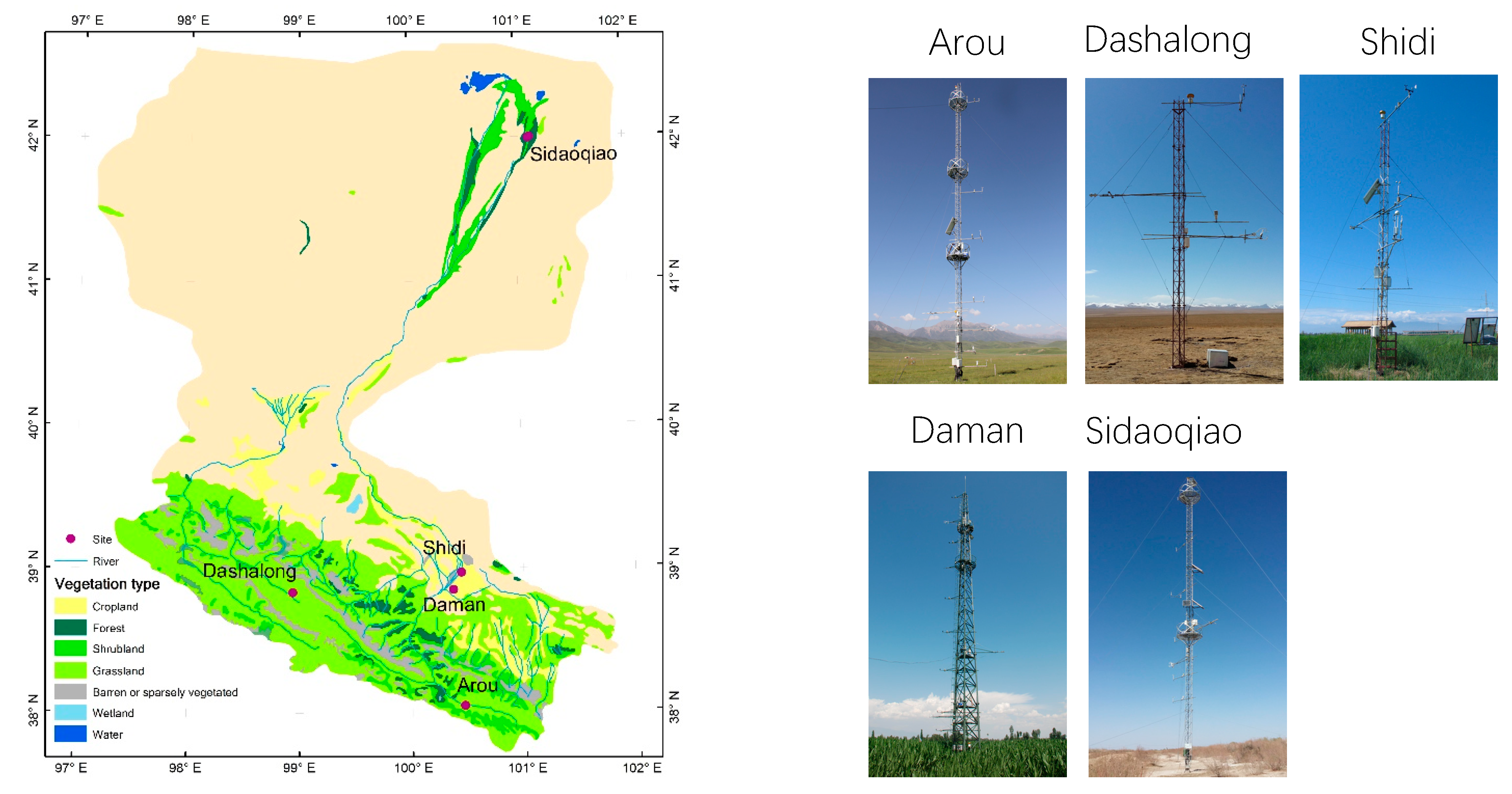
2.1. Study Area

The Heihe River Basin is the second-largest inland river basin in China and is located in the northwest arid region of China. The elevation ranges from 5300 m upstream to 900 m downstream. It contains diverse landscapes, such as glaciers, permafrost, alpine steppe/meadow, and forests in the upstream and irrigated croplands, riparian vegetation, wetlands, and gobi desert in the middle stream and downstream [12]. An EC measurement network was established in 2013 in the Heihe River Basin [13,14]. The flux between the ecosystem and the atmosphere and ancillary meteorological variables were measured in the dominant vegetation types of this region. The measured data was collected from five sites from 2014 to 2015. The detailed information of these sites is listed in

Table 1. Information of the Eddy Covariance (EC) sites in the Heihe River Basin.

Site Name	Land Cover	Latitude	Longitude	Elevation (m)
Arou	Grassland	38.0473	100.4643	3033
Dashalong	Grassland	38.8399	98.9406	3739
Daman	Cropland (Maize)	38.85551	100.3722	1556
Shidi	Wetland	38.97514	100.4464	1460
Sidaoqiao	Shrubland	42.0012	101.1374	873

, while the spatial distribution of these sites is shown in Figure 1. The Arou site and the Dashalong site are located in the upstream, and the vegetation is the alpine meadow. The Daman site and the Shidi site are located in the middle stream, and the vegetation is maize (cropland) and reed (wetland), respectively. The Sidaoqiao site is located in the riparian zone of the downstream, and the vegetation at this site is tamarisk.

The EC measured 10 Hz data was processed using despike, coordinate rotation, frequency response correction, and WPL correction to obtain the half-hourly data [15]. Then the half-hourly EC data was gap-filled and partitioned into the GPP and ecosystem respiration using the REddyProc package (https://cran.r-project.org/web/packages/REddyProc (accessed on 10 January 2019)) [16] in the R environment. The measured air temperature, downward shortwave radiation, relative humidity, soil moisture, and GPP daily value were used to force or validate the LUE model. The MODIS reflectance at these sites was extracted from the MOD09A1 collection 6. The normalized difference vegetation index (NDVI), the enhanced vegetation index (EVI), and the land surface water index (LSWI) were calculated from the MODIS reflectance data at these sites.

2.2. LUE Models

The LUE model is an effective tool to estimate the GPP using remote sensing data. LUE models can be generalized as the following formula:

$$\mathrm{GPP} = \mathrm{FAPAR} \times \mathrm{PAR} \times LU{E}_{max}\times \mathrm{f}(\mathrm{T}, \mathrm{S}, ---)$$

(1)

where FAPAR is the fraction of absorbed photosynthetically active radiation (PAR). $LU{E}_{max}$ is the maximum light using efficiency, and f(T, S, ---) is an environmental scalar on the photosynthesis rate. According to different schemes to quantify the environmental stress on photosynthesis, many LUE models have been developed. In this study, five widely used LUE models were selected to simulate the GPP seasonal dynamic at dominant vegetation types of the study area. They were Global Production Efficiency Model (GLO-PEM) [17], Vegetation Photosynthesis Model (VPM) [18], Carbon fixation model (C-Fix) [5], Eddy Covariance-Light Use Efficiency (EC-LUE) [6], and MODIS GPP product algorithm (MODIS-PSN) [7]. All the models were forced using in-situ measured meteorological data and default parameters for each site. Information regarding these models is listed in

Table 2. The Light Use Efficiency (LUE) models used in this study.

Model	Main Formula	Input Variables
GLO-PEM	GPP = APAR × LUEmax× f(T) × f(SM) × f(VPD)	PAR, NDVI, T, SM, VPD
VPM	GPP = APAR × LUEmax× f(T) × f(LSWI) × f(P)	PAR, EVI, T, LSWI
C-Fix	GPP = APAR × LUEmax× f(T) × f(CO2)	PAR, NDVI, T, CO2
EC-LUE	GPP = APAR × LUEmax× f(T) × f(EF)	PAR, NDVI, T, EF
MODIS-PSN	GPP = APAR × LUEmax× f(TMIN) × f(VPD)	PAR, NDVI, TMIN, VPD

T: air temperature; SM: soil moisture; VPD: vapor pressure deficit; EF: evaporative fraction.

.

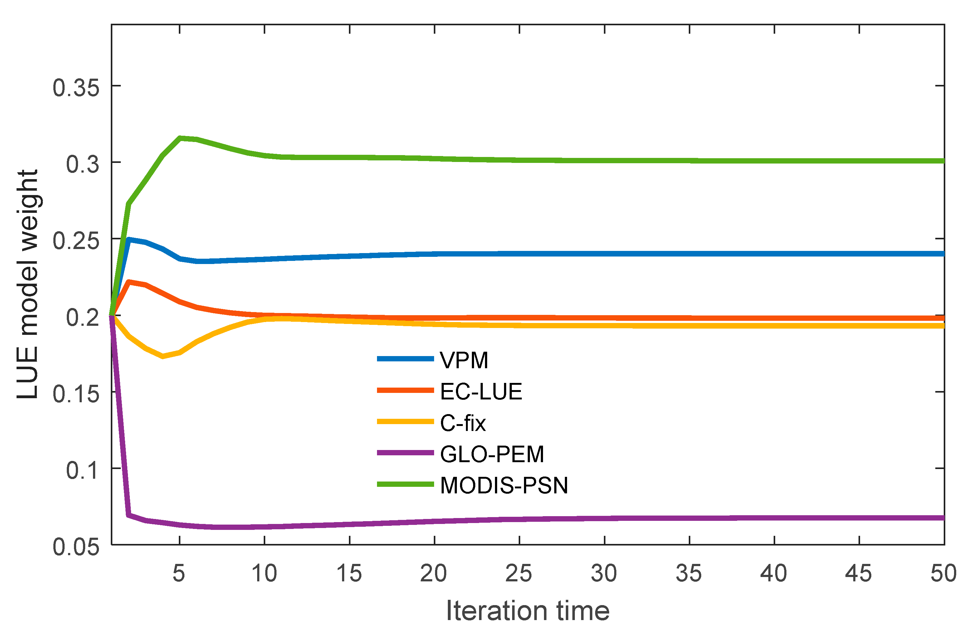
2.3. Bayesian Model Averaging

Bayesian model averaging is a scheme for the integration of outputs from multiple models. More detail regarding the theory can be found in the literature [10]. In the BMA method, the posterior distribution of the simulation variable, y, can be calculated using the following expression:

$$p\left(y|D\right)={\displaystyle \sum }_{i=1}^{k}p(fi|D)p_i(y|f_i,D)$$

(2)

where y is the variable to be simulated, $D=\left[y_1^{obs},y_2^{obs},\cdots ,y_T^{obs}\right]$ is the training data with length T, $f=\left[f_1,f_2,\cdots ,f_k\right]$ is the ensemble of outputs from k different models, $p(f_i|D)$ is the posterior probability of a simulation given the observation D, and $p_i\left(y|f_i,D\right)$ is the posterior distribution of y given the model simulation $f_i$ and the observed dataset D.

Finally, the posterior mean is estimated using the following formula:

$$E\left[y|D\right]={\displaystyle \sum }_{i=1}^{k}p(f_i|D)·E\left[p_i\left(y|f_i,D\right)\right]={\displaystyle \sum }_{i=1}^k{w}_i\left(a_i+b_i{f}_i\right)$$

(3)

where $w_i$ is the weight for model i and ${{\displaystyle \sum }}_{i=1}^k{w}_i=1$; $a_i$ and $b_i$ are bias correction terms that are derived using a simple linear regression of y on $f_i$.

Measurements obtained from the five sites in 2014 were used to train the BMA method, and measurements obtained in 2015 were used to validate the performance of the BMA method.

2.4. Model Accuracy Evaluation

The determinant coefficient, R², and the root mean square error (RMSE) were used to evaluate the model performance. The formulas for R² and the RMSE are as follows:

$$R^2=1-\frac{{{\displaystyle \sum }}_{i=1}^n{\left(P_i-O_i\right)}^2}{{{\displaystyle \sum }}_{i=1}^n{\left(O_i-\overline{O}\right)}^2}$$

(4)

$$RMSE=\sqrt{\frac{1}{N}{\displaystyle \sum }_{i=1}^n{\left(P_i-O_i\right)}^2}$$

(5)

where $P_i$ is the simulated GPP, $O_i$ is the EC-measured GPP in this study,$\overline{O}$ is the average of all the measurements, and N is the number of measurements.

3. Results

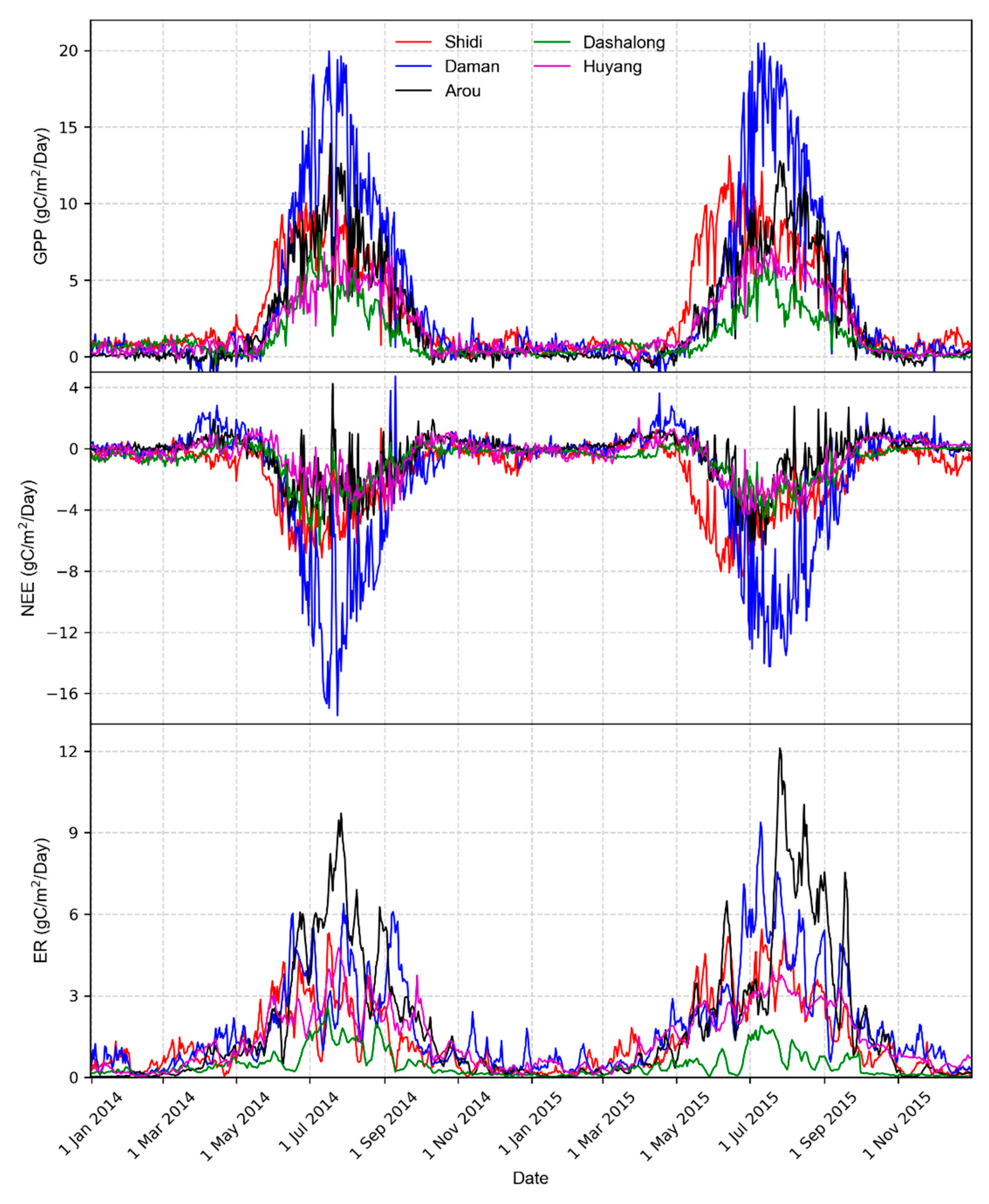
3.1. Carbon Flux Dynamics in the Heihe River Basin

The seasonal carbon flux dynamics of the five dominant vegetation types in the Heihe River Basin are shown in Figure 2. The annual carbon flux is summarized in

Table 3. Annual carbon flux at the five study sites in the Heihe River Basin.

Site Name	GPP (gC/m2/yr)		NEE (gC/m2/yr)		ER (gC/m2/yr)
	2014	2015	2014	2015	2014	2015
Arou	845.90	879.63	−175.61	−112.54	670.29	767.08
Dashalong	506.58	449.24	−314.61	−305.16	191.97	144.08
Daman	1329.96	1397.60	−726.94	−648.23	603.02	749.36
Shidi	1008.57	1165.77	−559.52	−609.76	449.05	556.02
Sidaoqiao	664.82	753.58	−190.00	−211.96	474.82	541.62

. Carbon flux at these sites had an obvious seasonal cycle. The carbon flux began increasing in early May, reached the maximum in July and returned to the minimum in later October (Figure 2). Alpine grassland is the dominant vegetation type in the upper stream of the study area. Both Arou and Dashalong are covered with alpine grass. From the carbon flux measurement, the annual GPP was 862.76 gC/m²/year at Arou and 477.91 gC/m²/year at Dashalong. The annual Net Ecosystem Exchange (NEE) was −144.08 gC/m²/year at Arou and −309.89 gC/m²/year at Dashalong. The annual Ecosystem Respiration (ER) was 718.69 gC/m²/year at Arou and 168.02 gC/m²/year at Dshalong. Artificial and natural oases are the dominant landscapes in the middle stream of the Heihe River Basin. Carbon flux at two sites in the oases, a cropland (Daman) and a wetland (Shidi), was measured. In the middle stream, the annual GPP for the cropland was 1364 gC/m²/year and 1087 gC/m²/year for the wetland, the annual NEE for the cropland was −688 gC/m²/year and −585 gC/m²/year for the wetland, and the annual ER for the cropland was 676 gC/m²/year and 502 gC/m²/year for the wetland. Natural oasis dominates the vegetated area in the downstream of the study area. The Sidaoqiao site is located in the natural oasis region of the downstream. The vegetation type is tamarisk at the Sidaoqiao site. This site is close to the main river channel. At the Sidaoqiao site, the annual GPP was 709 gC/m²/year, the annual NEE was −201 gC/m²/year, and the annual ER was 508 gC/m²/year. All of these sites were carbon sinks and absorbed more than 100 gC/m²/year.

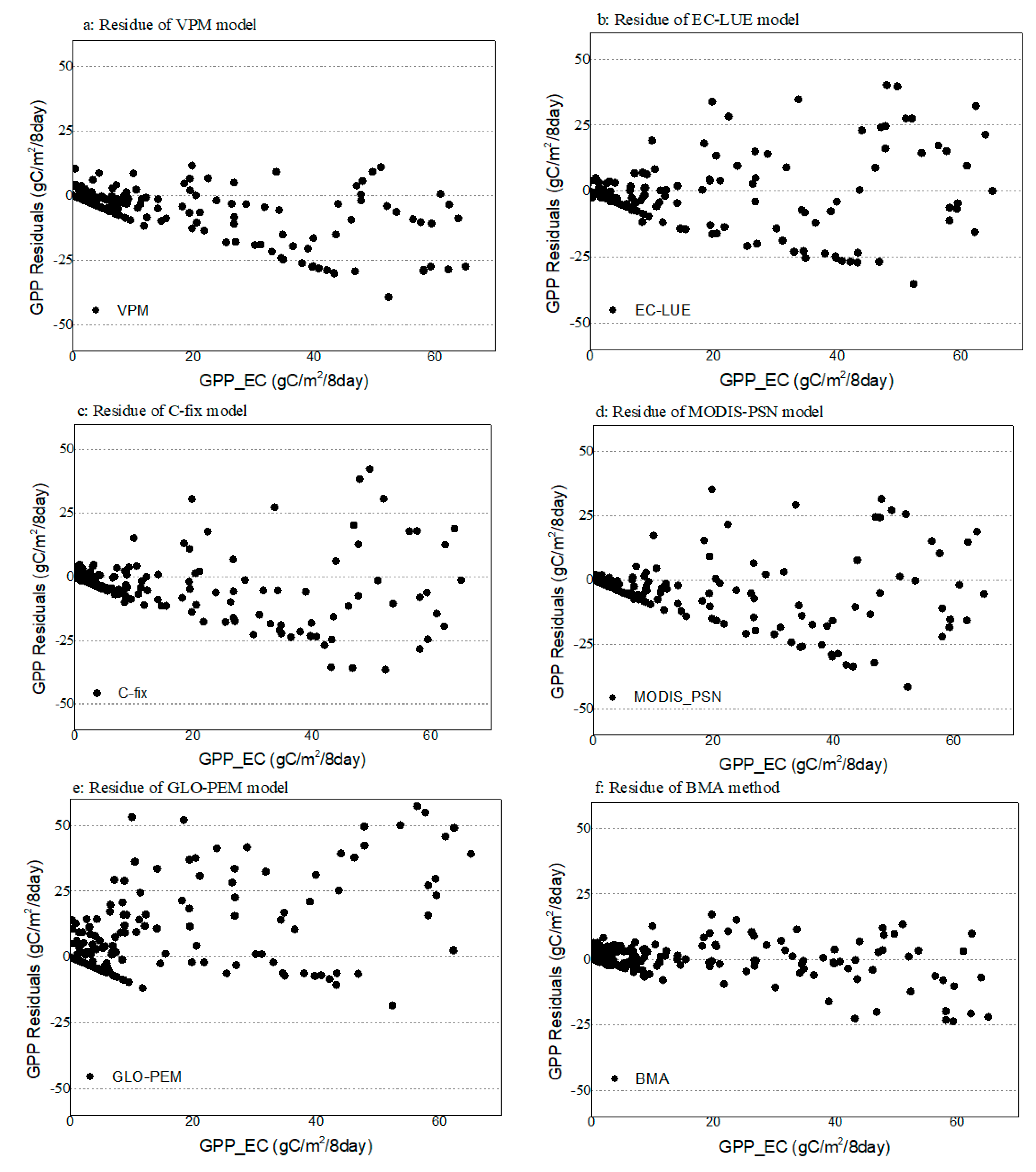
3.2. The BMA Based GPP Estimation

The determinant coefficient and RMSE were calculated between the simulated GPP and the EC-measured GPP (

Table 4. Determinant coefficients and RMSEs between the simulated GPP and the EC-measured GPP. (Data measured during 2014/2015 was used to train/validate the BMA method. The highest R² and the smallest RMSE were bolded.).

Site		R2						RMSE (gC/m2/8 day)
		VPM	EC-LUE	C-Fix	GLO-PEM	MODIS_PSN	BMA	VPM	EC-LUE	C-Fix	GLO-PEM	MODIS_PSN	BMA
Arou	Training	0.95	0.95	0.95	0.95	0.97	0.96	6.7	8.1	8.4	26.0	6.0	4.8
	Validation	0.95	0.94	0.94	0.94	0.95	0.95	10.1	7.0	10.9	23.8	10.3	6.9
Dashalong	Training	0.83	0.79	0.73	0.79	0.79	0.8	8.8	7.1	10.7	10.9	9.6	6.0
	Validation	0.88	0.91	0.84	0.82	0.76	0.87	7.1	3.9	8.2	13.2	8.4	4.7
Daman	Training	0.95	0.94	0.95	0.94	0.96	0.95	11.5	13.6	9.6	23.9	10.9	8.4
	Validation	0.96	0.96	0.97	0.95	0.98	0.97	15.7	8.4	8.2	41.5	6.7	8.6
Shidi	Training	0.83	0.85	0.87	0.81	0.82	0.84	9.9	15.5	14.7	39.5	13.6	8.6
	Validation	0.75	0.82	0.79	0.83	0.82	0.81	18.4	16.1	17.0	40.9	13.5	15.1
Sidaoqiao	Training	0.93	0.91	0.94	0.93	0.91	0.95	5.7	7.2	4.8	24.3	8.5	3.4
	Validation	0.85	0.84	0.87	0.85	0.78	0.87	9.3	9.7	7.4	25.7	11.6	7.6
All sites	Training	0.90	0.90	0.90	0.89	0.90	0.91	9.5	11.0	10.2	21.6	10.8	5.8
	Validation	0.88	0.90	0.89	0.88	0.85	0.90	12.7	9.9	10.9	25.1	11.3	8.1

). As expected, the results from the trained BMA method had the highest accuracy. Averaging the R² and RMSE among all of the sites indicated that BMA had the highest R² and the lowest RMSE among all the models during the training and validation stages (Table 4). However, if one looks at one of the five sites, the BMA was not always the highest-accuracy method, and some LUE models performed better than the BMA. The LUE models performed differently at different sites. At a specific site, the performance of the LUE models varied greatly. For example, the R² of the C-fix model in 2014 at the Dashalong site was 0.73, but the R² was 0.97 in 2015 at the Daman site. At the Arou site, the MODIS-PSN model performed better than other LUE models, but the C-fix model performed better than other LUE models at the Sidaoqiao site. Overall, at each site, the BMA method was close to the best one of the LUE models. To further explore the performance of these methods, the residual is plotted for each method (Figure 3). The residuals of the BMA method were uniformly distributed around 0 and were less than the standard deviation (SD) of the measurements. The residuals of the BMA method were smaller than all the LUE models. All the LUE models had values outside the 1x standard deviation range. Even GLO-PEM and EC-LUE had values outside the 2x standard deviation range. The convergence trajectory of the coefficients for LUE models at the Arou site is shown in Figure 4. The initial coefficients for each LUE model were assigned a fixed value, and the value changed during the iteration and quickly reached a steady-state (Figure 4).

4. Discussion

The high spatial heterogeneity of GPP is an obstacle to accurately obtain regional GPP. We found that the carbon flux obtained using the eddy covariance method varied greatly among the different vegetation types. The artificial oasis dominated by croplands showed the highest GPP and carbon sequestration capacity. This indicates that both natural factors and human activity have a great impact on carbon flux and cannot be neglected. Eddy covariance is one of the commonly used techniques to measure ecosystem-scale carbon flux, but still it involves many uncertainties that should be noted when analyzing the data. The uncertainties primarily result from three aspects. First, the eddy covariance data quality is affected by sensor configurations and meteorological conditions [19]. Hence, strict quality control is required for the raw data before its use. Second, due to instrument malfunction and spikes, data gaps are inevitable in the raw data, and gap-filling is a necessary step to obtain continuous carbon flux [20]. This process also leads to uncertainties in the results. Third, the eddy covariance method only directly measures the NEE, and the GPP and ER are partitioned from the NEE with some hypothesis, a fact that can also result in uncertainties in the GPP and ER [21,22].

The LUE model performance changed greatly with vegetation types. The LUE model is a widely used method to estimate the GPP, especially at the regional scale. However, GPP simulated using the LUE model contains uncertainties that result from the model parameters, meteorological input data, and remote sensing input data [23,24]. Model parameters vary with species and vegetation community compositions, and the LUE models usually only provide default parameters for the major vegetation types. When applying the LUE models in a small region, the default parameters may result in great uncertainties. The uncertainties that result from meteorological input data are primarily caused by gap filling and the interpolation of measured data. Remote sensing input data (such as FPAR, NDVI, EVI, LSWI and others) in the LUE model also contain uncertainties that result from bad data quality [25]. Some studies reported that model parameters have a larger impact on the simulation accuracy than the meteorological input data and remote sensing input data [26].

BMA is an effective method to improve modeling accuracy. Every model has some limitations caused by its hypothesis and parameterization scheme [27]. The average of multiple model outputs can overcome this problem and be thought of as more reliable than a single model output. In many studies, the classical average of a model ensemble has been used to conduct the research [28,29]. BMA provides a way to obtain the model ensemble weighted average [30]. By training the BMA method with measurement data, different weights are assigned to different models, and the weights also vary with spatial and vegetation type changes. This is more reasonable than the classical average because the performances of the LUE models are different at different locations and with different vegetation types [31,32]. Many studies have reported that BMA can improve the simulation accuracy than the classical average in stream-flow forecasting models [33] and evapotranspiration models [11]. This is consistent with the finding of the current study, where the RMSE of the BMA method was 5.8 gC/m²/8 day during the training period and 8.1 gC/m²/8 day during the validation period, while the classical averages were 12.6 gC/m²/8 day and 13.98 gC/m²/8 day, respectively. This demonstrates that BMA has the potential to improve GPP estimation by integrating multiple LUE models. Meanwhile, training process is vital to BMA application. The short data period for BMA training may result in some uncertainties in the simulation in this study. The training data should be as comprehensive as possible. Additionally, BMA is also able to calculate the uncertainties in its estimated GPP, which is useful when conducting the analysis with remote sensed GPP. In this study, we take the Heihe River Basin as an example to demonstrate the performance of the BMA method. As a universal method, if BMA is well-calibrated at the global scale, it can integrate the global GPP products and output high quality global GPP estimation.

5. Conclusions

In this study, five LUE models and the multi-model ensemble method were evaluated using measured daily carbon flux and meteorological data in the Heihe River Basin. The measured carbon flux data indicate that the GPP varied greatly among the different ecosystems in the Heihe River Basin from upstream to downstream. The cropland and wetland in the middle stream had the highest carbon uptake capacities. Performance of the LUE models indicated that the LUE models contain uncertainties resulting from model parameters and model struct. Single LUE model performance is not robust in different vegetation types. The LUE models without parameter calibration exhibited great inconsistencies in GPP simulations. The BMA method is an effective tool to integrate multi-model ensemble output. The RMSE between the BMA-simulated GPP and EC-measured GPP was the smallest. The use of the BMA method allows for the combination of multiple LUE models to yield a high-accuracy GPP.

References

1. Beer, C.; Reichstein, M.; Tomelleri, E.; Ciais, P.; Jung, M.; Carvalhais, N.; Rödenbeck, C.; Arain, M.A.; Baldocchi, D.; Bonan, G.B.; et al. Terrestrial Gross Carbon Dioxide Uptake: Global Distribution and Covariation with Climate. Science 2010, 329, 834–838. [Google Scholar] [CrossRef] [Green Version]
2. Turner, D.P.; Ritts, W.D.; Cohen, W.B.; Gower, S.T.; Zhao, M.; Running, S.W.; Wofsy, S.C.; Urbanski, S.; Dunn, A.L.; Munger, J.W. Scaling Gross Primary Production (GPP) over boreal and deciduous forest landscapes in support of MODIS GPP product validation. Remote Sens. Environ. 2003, 88, 256–270. [Google Scholar] [CrossRef] [Green Version]
3. Yuan, W.; Cai, W.; Xia, J.; Chen, J.; Liu, S.; Dong, W.; Merbold, L.; Law, B.; Arain, A.; Beringer, J.; et al. Global comparison of light use efficiency models for simulating terrestrial vegetation gross primary production based on the LaThuile database. Agric. For. Meteorol. 2014, 192–193, 108–120. [Google Scholar] [CrossRef]
4. Baldocchi, D.; Falge, E.; Gu, L.; Olson, R.; Hollinger, D.; Running, S.; Anthoni, P.; Bernhofer, C.; Davis, K.; Evans, R.; et al. FLUXNET: A New Tool to Study the Temporal and Spatial Variability of Ecosystem-Scale Carbon Dioxide, Water Vapor, and Energy Flux Densities. Bull. Am. Meteorol. Soc. 2001, 82, 2415–2434. [Google Scholar] [CrossRef]
5. Veroustraete, F.; Sabbe, H.; Eerens, H. Estimation of carbon mass fluxes over Europe using the C-Fix model and Euroflux data. Remote Sens. Environ. 2002, 83, 376–399. [Google Scholar] [CrossRef]
6. Yuan, W.; Liu, S.; Zhou, G.; Zhou, G.; Tieszen, L.L.; Baldocchi, D.; Bernhofer, C.; Gholz, H.; Goldstein, A.H.; Goulden, M.L.; et al. Deriving a light use efficiency model from eddy covariance flux data for predicting daily gross primary production across biomes. Agric. For. Meteorol. 2007, 143, 189–207. [Google Scholar] [CrossRef] [Green Version]
7. Running, S.W.; Nemani, R.R.; Heinsch, F.A.; Zhao, M.; Reeves, M.; Hashimoto, H. A Continuous Satellite-Derived Measure of Global Terrestrial Primary Production. Bioscience 2004, 54, 547–560. [Google Scholar] [CrossRef]
8. Xiao, X.; Hollinger, D.; Aber, J.; Goltz, M.; Davidson, E.A.; Zhang, Q.; Moore, B. Satellite-based modeling of gross primary production in an evergreen needleleaf forest. Remote Sens. Environ. 2004, 89, 519–534. [Google Scholar] [CrossRef]
9. Ballantyne, A.; Smith, W.; Anderegg, W.; Kauppi, P.; Sarmiento, J.; Tans, P.; Shevliakova, E.; Pan, Y.; Poulter, B.; Anav, A.; et al. Accelerating net terrestrial carbon uptake during the warming hiatus due to reduced respiration. Nat. Clim. Chang. 2017, 7, 148–152. [Google Scholar] [CrossRef]
10. Duan, Q. Multi-model ensemble hydrologic prediction using Bayesian model averaging. Adv. Water Resour. 2007, 30, 1371–1386. [Google Scholar] [CrossRef] [Green Version]
11. Zhu, G.; Li, X.; Zhang, K.; Ding, Z.; Han, T.; Ma, J.; Huang, C.; He, J.; Ma, T. Multi-model ensemble prediction of terrestrial evapotranspiration across north China using Bayesian model averaging. Hydrol. Process. 2016, 30, 2861–2879. [Google Scholar] [CrossRef]
12. Li, X.; Li, X.; Li, Z.; Ma, M.; Wang, J.; Xiao, Q.; Liu, Q.; Che, T.; Chen, E.; Yan, G.; et al. Watershed Allied Telemetry Experimental Research. J. Geophys. Res. 2009, 114. [Google Scholar] [CrossRef] [Green Version]
13. Li, X.; Cheng, G.D.; Liu, S.M.; Xiao, Q.; Ma, M.G.; Jin, R.; Che, T.; Liu, Q.H.; Wang, W.Z.; Qi, Y.; et al. Heihe Watershed Allied Telemetry Experimental Research (HiWATER): Scientific Objectives and Experimental Design. Bull. Am. Meteorol. Soc. 2013, 94, 1145–1160. [Google Scholar] [CrossRef]
14. Liu, S.; Li, X.; Xu, Z.; Che, T.; Xiao, Q.; Ma, M.; Liu, Q.; Jin, R.; Guo, J.; Wang, L.; et al. The Heihe Integrated Observatory Network: A Basin-Scale Land Surface Processes Observatory in China. Vadose Zone J. 2018, 17. [Google Scholar] [CrossRef]
15. Zhang, Z.; Wang, W.; Ma, M.; Xu, Z.; Wu, Y.; Huang, G.; Tan, J. Data Processing and Product Analysis of Eddy Covariance Flux Data for WATER. Remote Sens. Technol. Appl. 2010, 25, 788–796. [Google Scholar]
16. Wutzler, T.; Lucas-Moffat, A.; Migliavacca, M.; Knauer, J.; Sickel, K.; Šigut, L.; Menzer, O.; Reichstein, M. Basic and extensible post-processing of eddy covariance flux data with REddyProc. Biogeosciences 2018, 15, 5015–5030. [Google Scholar] [CrossRef] [Green Version]
17. Prince, S.D.; Goward, S.N. Global Primary Production: A Remote Sensing Approach. J. Biogeogr. 1995, 22, 815–835. [Google Scholar] [CrossRef]
18. Xiao, X.; Zhang, Q.; Braswell, B.; Urbanski, S.; Boles, S.; Wofsy, S.; Moore, B.; Ojima, D. Modeling gross primary production of temperate deciduous broadleaf forest using satellite images and climate data. Remote Sens. Environ. 2004, 91, 256–270. [Google Scholar] [CrossRef]
19. Foken, T.; Wichura, B. Tools for quality assessment of surface-based flux measurements. Agric. For. Meteorol. 1996, 78, 83–105. [Google Scholar] [CrossRef]
20. Papale, D.; Reichstein, M.; Aubinet, M.; Canfora, E.; Bernhofer, C.; Kutsch, W.; Longdoz, B.; Rambal, S.; Valentini, R.; Vesala, T.; et al. Towards a standardized processing of Net Ecosystem Exchange measured with eddy covariance technique: Algorithms and uncertainty estimation. Biogeosciences 2006, 3, 571–583. [Google Scholar] [CrossRef] [Green Version]
21. LASSLOP, G.; REICHSTEIN, M.; PAPALE, D.; RICHARDSON, A.D.; ARNETH, A.; BARR, A.; STOY, P.; WOHLFAHRT, G. Separation of net ecosystem exchange into assimilation and respiration using a light response curve approach: Critical issues and global evaluation. Glob. Chang. Biol. 2010, 16, 187–208. [Google Scholar] [CrossRef] [Green Version]
22. Reichstein, M.; Falge, E.; Baldocchi, D.; Papale, D.; Aubinet, M.; Berbigier, P.; Bernhofer, C.; Buchmann, N.; Gilmanov, T.; Granier, A.; et al. On the separation of net ecosystem exchange into assimilation and ecosystem respiration: Review and improved algorithm. Glob. Chang. Biol 2005, 11, 1424–1439. [Google Scholar] [CrossRef]
23. Wang, X.; Ma, M.; Huang, G.; Veroustraete, F.; Zhang, Z.; Song, Y.; Tan, J. Vegetation primary production estimation at maize and alpine meadow over the Heihe River Basin, China. Int. J. Appl. Earth Obs. Geoinf. 2012, 17, 94–101. [Google Scholar] [CrossRef]
24. Wang, X.; Ma, M.; Li, X.; Song, Y.; Tan, J.; Huang, G.; Zhang, Z.; Zhao, T.; Feng, J.; Ma, Z.; et al. Validation of MODIS-GPP product at 10 flux sites in northern China. Int. J. Remote Sens. 2013, 34, 587–599. [Google Scholar] [CrossRef]
25. Wang, X.; Xiao, J.; Li, X.; Cheng, G.; Ma, M.; Che, T.; Dai, L.; Wang, S.; Wu, J. No Consistent Evidence for Advancing or Delaying Trends in Spring Phenology on the Tibetan Plateau. J. Geophys. Res. 2017, 122, 3288–3305. [Google Scholar] [CrossRef]
26. Wang, H.; Li, X.; Ma, M.; Geng, L. Improving Estimation of Gross Primary Production in Dryland Ecosystems by a Model-Data Fusion Approach. Remote Sens. 2019, 11, 225. [Google Scholar] [CrossRef] [Green Version]
27. Parrish, M.A.; Moradkhani, H.; DeChant, C.M. Toward reduction of model uncertainty: Integration of Bayesian model averaging and data assimilation. Water Resour. Res. 2012, 48. [Google Scholar] [CrossRef]
28. Zhang, Y.; Xiao, X.; Guanter, L.; Zhou, S.; Ciais, P.; Joiner, J.; Sitch, S.; Wu, X.; Nabel, J.; Dong, J.; et al. Precipitation and carbon-water coupling jointly control the interannual variability of global land gross primary production. Sci. Rep. 2016, 6, 39748. [Google Scholar] [CrossRef] [Green Version]
29. Dormann, C.F.; Calabrese, J.M.; Guillera-Arroita, G.; Matechou, E.; Bahn, V.; Bartoń, K.; Beale, C.M.; Ciuti, S.; Elith, J.; Gerstner, K.; et al. Model averaging in ecology: A review of Bayesian, information-theoretic, and tactical approaches for predictive inference. Ecol. Monogr. 2018, 88, 485–504. [Google Scholar] [CrossRef] [Green Version]
30. Raftery, A.E.; Gneiting, T.; Balabdaoui, F.; Polakowski, M. Using Bayesian Model Averaging to Calibrate Forecast Ensembles. Mon. Weather Rev. 2005, 133, 1155–1174. [Google Scholar] [CrossRef] [Green Version]
31. Wu, C.; Munger, J.W.; Niu, Z.; Kuang, D. Comparison of multiple models for estimating gross primary production using MODIS and eddy covariance data in Harvard Forest. Remote Sens. Environ. 2010, 114, 2925–2939. [Google Scholar] [CrossRef]
32. Sun, Z.; Wang, X.; Zhang, X.; Tani, H.; Guo, E.; Yin, S.; Zhang, T. Evaluating and comparing remote sensing terrestrial GPP models for their response to climate variability and CO2 trends. Sci. Total Environ. 2019, 668, 696–713. [Google Scholar] [CrossRef] [PubMed]
33. Vrugt, J.A.; Diks, C.G.H.; Clark, M.P. Ensemble Bayesian model averaging using Markov Chain Monte Carlo sampling. Environ. Fluid Mech. 2008, 8, 579–595. [Google Scholar] [CrossRef]
Figure 1. Distribution of the study sites in the Heihe River Basin.
Land 10 00329 g001
Figure 2. Seasonal carbon flux dynamics at the five study sites.
Land 10 00329 g002
Figure 3. Residual plots of different models at the five sites (a: VPM; b: EC-LUE; c: C-fix; d: MODIS-PSN; e: GLO-PEM; f: BMA). The dashed line is the 1*SD and 2*SD (SD = 25 gC/m2/8 day for the GPP measurement at Arou site).
Land 10 00329 g003
Figure 4. The weights convergence trajectory of the LUE models during the BMA method training.
Land 10 00329 g004