Infrastructure Investment and Regional Economic Growth: Evidence from Yangtze River Economic Zone

Abstract

To better understand the impacts of infrastructure investment on economic growth and, we used Cobb-Douglas production function model to develop the stock of public infrastructure capital into the economic growth model. It applies spatial panel data model effect analysis to statistical data of the Yangtze River Economic Zone with 131 cities from 2003 to 2016 and investigates the relationship between different types of public infrastructure capital stock and regional economic growth in different periods. The empirical results show that (1) the economic growth of the cities in the Yangtze River Economic Zone has characteristics of significant spatial dependence, the degree and significance of spatial dependence are gradually declining, and the spatial agglomeration of the economic growth in the cities in the region is relatively stable. (2) Different types of public infrastructure capital stock have distinct spatial effects on regional economic growth. The capital stock of energy infrastructure significantly promotes global economic growth. The capital stock of transportation infrastructure significantly stimulates the local economic growth and inhibits the economic growth of the adjacent areas. The capital stock of water-related infrastructure restrains local economic growth and promotes economic growth in adjacent areas. These findings indicate that increasing investment in public infrastructure development in the Yangtze River Economic Zone remains an effective measure to promote regional economic growth. Under the premise of limited resources, taking full account of the effects of various types of investment can promote the mutual benefit of the economies in the region and effectively achieve the strategic objectives for the Yangtze River Economic Zone.

1. Introduction

Infrastructure development can effectively promote economic growth is an important experience for governments to formulate economic growth policies in the last 100 years [1,2]. The international financial crisis in 2008 has had a huge negative impact on the economic growth of all countries in the world. The rising unemployment rate, economic recession, and the reduction of living standards are bothering people all over the world [3]. To this end, in order to expand domestic demand and stimulate economic growth, the Chinese government launched a “four trillion” public infrastructure investment and construction project, which played an important role in alleviating the impact of the financial crisis. However, while making great achievements in large-scale infrastructure investment and construction, we should also recognize that this kind of short-term large-scale infrastructure investment and construction will further enlarge the degree of imbalance of social and economic growth among different regions [4,5,6]. Therefore, since the “12th Five Year Plan”, the Chinese government has put forward the economic strategy of “transformation, structural adjustment and stable growth” objectives. In this context, the construction of the “Yangtze River Economic Zone” has become a national strategy, and it is clearly pointed out that it is necessary to improve the function of the Yangtze River golden waterway and build a comprehensive three-dimensional transportation corridor. The construction of public infrastructure represented by large-scale projects such as “West to East Gas Transmission”, “West to East Power Transmission”, not only promotes the regional economic integration, but also improves the efficiency of factor flow, which is also the practical basis and important means to realize the strategic goal of the construction of the Yangtze River Economic Zone.

The relationship between infrastructure and economic growth has, in recent years, become one of the most important economic topics in both academic and policy circles. In the 1940s, Rosenstein-Rodan, a Polish-born British economist, put forward the theory of “Great Promotion” [7]. He believed that the public infrastructure industry was the leading capital whose accumulation would lead to economic growth, and therefore that only by strengthening infrastructure investment could the overall and balanced development of the national economy be promoted, and the vicious circle of poverty left behind. The classical Cobb-Douglas production function model was used to quantitatively study the decline of public infrastructure investment and productivity in the United States during 1949–1985 [8,9]. The authors proposed the categories of “core” infrastructure (expressway, public transport network, power energy facilities, water supply, sewage, etc.) and demonstrates the impact of public infrastructure investment on productivity. The promotion of such core infrastructure has a significant positive impact, and the marginal rate of return is higher than that of private sector investment, with an output elasticity of 0.39. This concept has been met with considerable criticism; relevant studies suggest that there may be pseudo-correlation between Aschauser’s findings and the variables of time series data used by similar research institutes and that the differences among cross-sectional data are not considered in the model. Therefore, some scholars turn to provincial and state panel data for analysis [5,6,10,11,12].

With the development of new geo-economics, the focus of research concerning infrastructure investment has gradually changed from the direct output effect to the spatial effect of promoting the flow of production factors. Cantos finds evidence of a spatial spillover effect of transport infrastructure on economic growth by analyzing the total investment and social output of newly constructed transport infrastructure in Spain [13]. Bonaglia studies the impact of different types of public infrastructure investment on total factor productivity across Italy and finds that different types of public infrastructure investment have different impacts on total factor productivity [14]. Furthermore, Boarnet finds evidence that public infrastructure development may have negative spatial effects [15]. According to these studies, public infrastructure plays a connecting role, linking many regions into a whole through tangible or intangible means. While infrastructure makes factors of production more convenient to economically developed areas through the agglomeration effect, it also improves the technological level of production in the surrounding areas through a diffusion effect as regions with faster growth drive the development of regions with slower growth through positive spatial spillover effects. However, infrastructure may also allow the flow of economic growth to one region to the detriment of economic growth in the surrounding areas.

Moderately advanced infrastructure development can effectively improve the level of economic growth; China’s economic growth demonstrates the importance of infrastructure, as confirmed by empirical studies. Based on panel data for 24 provinces (cities) in China from 1985 to 1998, Démurge empirically analyses the relationship between geographical location, economic policy and economic growth and found that geographical location and the level of transportation infrastructure development were the main reasons for the unbalanced development among regions [16]. Using panel data for 31 provinces (cities) and autonomous regions in China from 1993 to 2014, Li and Dong empirically demonstrate the relationship between infrastructure investment scale and economic growth, indicating that there is an inverted U-shaped relationship between infrastructure investment and economic growth [3] and that the three major economic blocks of Eastern, Central and Western China are at different stages of development. This finding indirectly confirms the views of Bougheas [17] and others: infrastructure investment can promote economic growth but with decreasing returns to scale. Based on a series of studies on the relationship between transportation infrastructure and economic growth in different regions of China, it is found that the output resilience of China’s transport infrastructure to regional economic growth is positive, and the spatial spillover effect is strongly significant [18,19,20]. However, the spatial spillover effect may be positive or negative. If the spatial spillover effect is not taken into account, the impact of transportation infrastructure on regional economic growth will be overestimated [21]. The above analysis generally tends to agree that public infrastructure development in China will promote economic growth in specific regions. However, after the Chinese government launched a large-scale investment plan for infrastructure development in 2008, some Chinese scholars put forward different opinions according to the actual operation of China’s economy. These scholars believed that providing an excessive supply of infrastructure development in areas with a backward industrial development level will have a “crowding-out effect” on other types of investment (such as human capital investment). At the same time, unreasonable factor input will reduce the allocation efficiency of investment, which will have a negative impact on economic growth.

In summary, infrastructure development and economic growth have a relatively complex relationship. First, as an important macro-control policy means, public infrastructure investment has a direct pull effect on the regional economy, which can be directly reflected in its contribution to GDP. Second, public infrastructure investment has a spatial spillover effect, which can have a positive or negative impact on technology spillover, industrial docking, factor mobility efficiency and other aspects of regional economies. Third, the path and the degree of the impact of infrastructure development on economic growth differ by industry. Existing studies focus on the impact of infrastructure investment on economic growth but lack discussion on the spatial effects of different types of public infrastructure investment on economic growth over a certain period of time in the same region. The contribution of this research bridges the gap by taking spatial correlation factors into account in spatial econometric analysis and adopting the Yangtze River Economic Zone as the research object for the analysis of the relationship between economic growth and the investment stock of different types of public infrastructure development.

This paper is presented in three sections. Section 1 explains the data sources and methods. Section 2 presents results and discussions. Section 3 makes a conclusion with policy and practice implications.

2. Methodology

2.1. Study Area

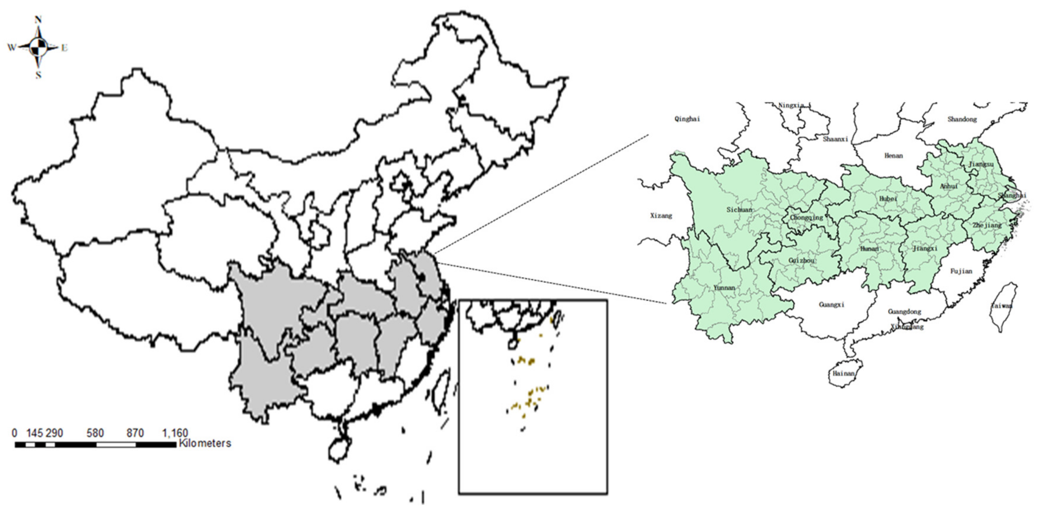
The Yangtze River Economic Zone covers 11 provinces with 131 cities, namely, Shanghai, Jiangsu, Zhejiang, Anhui, Jiangxi, Hubei, Hunan, Chongqing, Sichuan, Yunnan and Guizhou. We choose Yangtze River Economic Zone with three reasons: (1) region demographics, (2) geographical location and (3) selected as national economic development zone. Yangtze River Economic Zone covers an area of approximately 2.05 million square kilometers, accounting for 21% of China’s total area, and its population and economy represent more than 40% of the country’s total population and GDP. Spanning the eastern, central and western parts of China, the region holds an important geographical position and has always played a relatively active part in China’s national economic growth. Before 2014, there were no official plan for Yangtze River Economic Zone and its development has been overlooked (no official announcement but does exist and known for public). In September 2014, the Chinese government put forward the basic concept of building the Yangtze River Economic Zone. In September 2016, the Outline of the Development Planning of the Yangtze River Economic Zone was officially issued, making the zone a key area for future government investment in public infrastructure development (Figure 1).

2.2. Test of Spatial Dependence

Spatial correlation refers to the potential interdependence of some variables between the observed data in the same distribution area. It is generally measured by the Moran index, divided into the global Moran index and the local Moran index. The global index considers the whole and judges whether there is spatial agglomeration, and the local index identifies the agglomeration area.

The formula for calculating the global Moran index is as follows:

$$Mora{n}^{\prime }s I=\frac{{{\displaystyle \sum }}_{i=1}^n{{\displaystyle \sum }}_{j\ne i}^n{W}_{ij}\left(y_i-\overline{y}\right)\left(y_j-\overline{y}\right)}{S^2{\displaystyle {\displaystyle \sum }_{i=1}^n}{{\displaystyle \sum }}_{j\ne i}^n{W}_{ij}}$$

(1)

The formula for calculating the local Moran index is as follows:

$$local Mora{n}^{\prime }s I=\frac{\left(y_i-\overline{y}\right)}{S^2}{{\displaystyle \sum }}_{j=1}^n{w}_{ij}\left(y_j-\overline{y}\right)$$

(2)

Among them, $n$ is the number of regions, $y_i$ is the observation value of region $ii$,$\overline{y}$ is the average observed value of the tested variables. $S^2$ is the sample variance with n-1 degrees of freedom and $W_{\mathit{ij}}$ is the element value of spatial weight matrix $W$. Many methods are used to construct the spatial weight matrix [22]. Consideration of geographical objectivity, this paper selects: (1) Spatial weight matrix based on the co-edge adjacency rook 0–1 configuration is selected since there is no connection in vertices. We choose rook as we are discussing the impacts to the neighborhood cities. (2) Spatial weight matrix of geographical distance (the linear distance between the administrative centers of the two regions) is for spatial analysis. The global Moran index $Mora{n}^{\prime }s I$ is between −1 and 1. When the exponent is greater than 0, the data show positive spatial correlation, and the larger the value is, the more obvious the spatial correlation. When the index is less than 0, the data show negative spatial correlation, and the smaller the value is, the greater the spatial difference. When the index is 0, the space is random.

We need to test the significance of $Mora{n}^{\prime }s I$. Considering its approximately normal distribution, we can use $Z$ statistics to test its significance: $Z=\frac{\left(I-E\left(I\right)\right)}{\sqrt{VER\left(I\right)}}$.

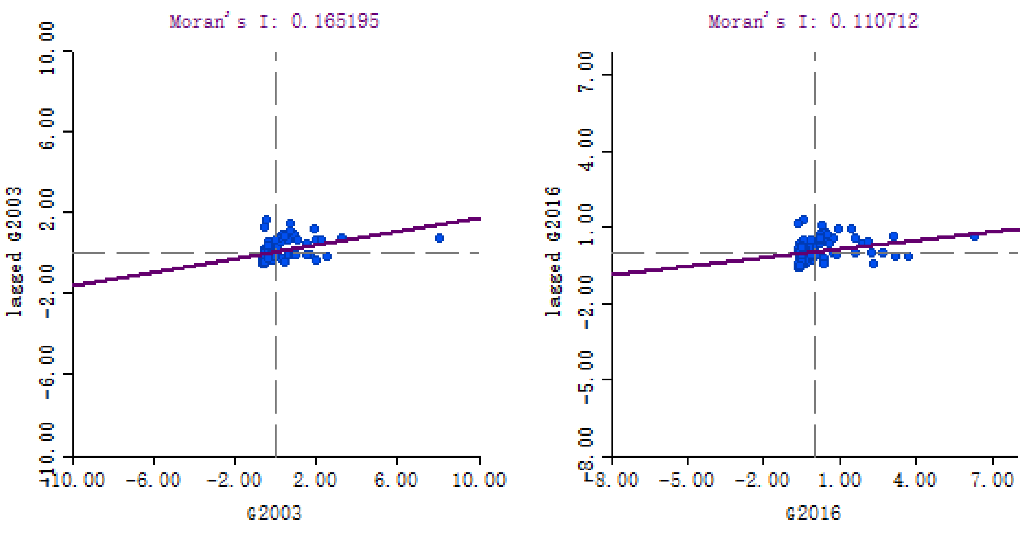
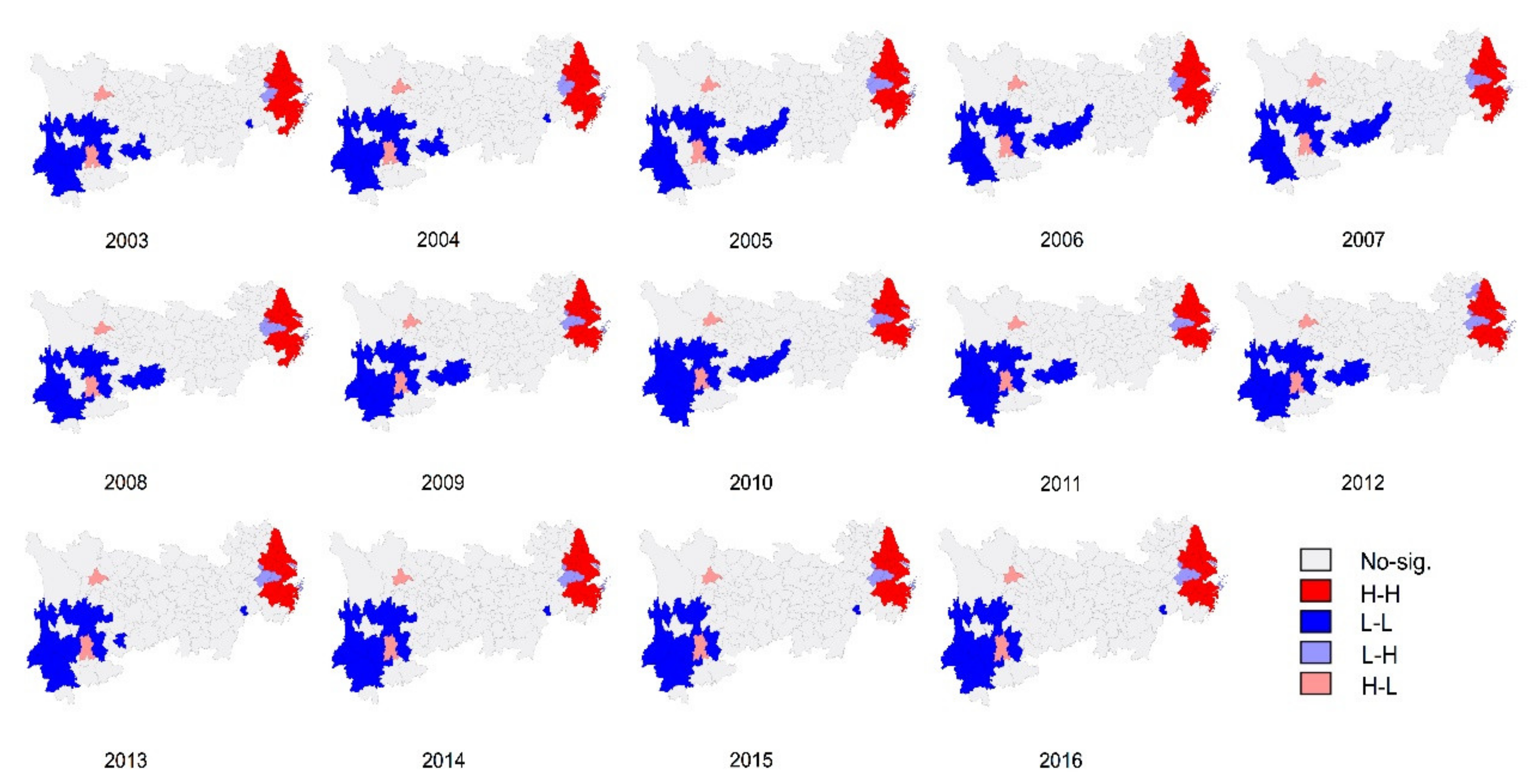
The global Moran index is the average value of the local Moran index statistics. If the distribution of local statistics is not uniform, there will be some deception in the overall display. Therefore, after calculating the global Moran index, the local Moran index is calculated to discriminate among the spatial agglomeration of the research objects in the region. A scatter plot of the local Moran indexes can reflect the spatial agglomeration of the real GDP of each city.

2.3. Construction and Selection of the Spatial Econometric Model

To analyze the impact of the stock of public infrastructure investment on regional economic growth, this section mainly refers to the capital splitting method of Zhang [20] on the basis of the Boarnet model [15].

First, the stock of fixed assets in the whole society is divided into two categories: public sector investment $K_g$ and private sector investment $K_s$. Then, the public sector $K_g$ is decomposed into public infrastructure development capital stock $K_{inf}$ and public non-productive investment capital stock $K_p$ [4,23], and a regional economic growth model including public infrastructure variables is established. The real GDP of each region is as Formula (3):

$$Y=A\varphi \left(K_{inf}\right)\phi \left(K_p\right)f\left(K_s,L,X\right)$$

(3)

$Y$ is the total output, $A$ is the coefficient of technological progress, $K_{inf}$ is the capital stock of public infrastructure development, $K_s$ is the capital stock of private sector investment, $K_p$ is the stock of other public sector investment except for the investment stock of public infrastructure development, $L$ is the labour input, and $X$ is the vector of various factors affecting total output, including human capital accumulation, urbanization level, and market openness. The scale of government expenditure and other new economic growth and new economic geography factors, $\varphi$ and $\phi$, represent the spatial relationship of specific independent variables. By integrating Formula (3), a production function model Formula (4) including various types of capital stock is obtained.

$$Y=Af\left(L,K_{inf},K_p,K_s,X\right)$$

(4)

To further explore the impact of different types of public infrastructure development on economic growth $K_{inf}$ is divided into $K_{energy},K_{transport},K_{water}$, and formula (4) is expanded to obtain the following formula:

$$Y=Af\left(K_{energy},K_{transport},K_{water},K_s,K_p,L,X\right)$$

(5)

A general panel regression model (OLS model) is obtained by expanding model (5) to the logarithmized configuration based on the Cobb-Douglas production function. See Formula (6).

$$\begin{gathered} \log \left(Y\right)=\alpha +{\beta }_1\log \left(L\right)+{\beta }_2\log \left(K_{energy}\right)+{\beta }_3\log \left(K_{transport}\right)+{\beta }_4\log \left(K_{water}\right) \\ +{\beta }_5\log \left(K_s\right)+{\beta }_6\log \left(K_p\right)+{\beta }_7\log \left(X\right)+\epsilon \end{gathered}$$

(6)

The main objective of this paper is to study the impact of public infrastructure on real GDP and its spillover effect. The model includes the endogenous interaction effect $W\log \left(Y\right)$ of explanatory variables, the exogenous interaction effect $W\log \left(K\right)$ between explanatory variables and the interaction effect $Wu$ of different units of interference. The OLS model is extended to a spatial econometric model as follows:

(1) Spatial autoregressive model (SAR)

$$\begin{gathered} \log \left(Y\right)=\alpha +\rho W\log \left(Y\right)+{\beta }_1\log \left(L\right)+{\beta }_2\log \left(K_{energy}\right)+{\beta }_3\log \left(K_{transport}\right) \\ +{\beta }_4\log \left(K_{water}\right)+{\beta }_5\log \left(K_s\right)+{\beta }_6\log \left(K_p\right)+{\beta }_7\log \left(X\right)+\epsilon \end{gathered}$$

(7)

(2) Spatial error model (SEM)

$$\begin{gathered} \log \left(Y\right)=\alpha +{\beta }_1\log \left(L\right)+{\beta }_2\log \left(K_{energy}\right)+{\beta }_3\log \left(K_{transport}\right)+{\beta }_4\log \left(K_{water}\right) \\ +{\beta }_5\log \left(K_s\right)+{\beta }_6\log \left(K_p\right)+{\beta }_7\log \left(X\right)+u \\ u=\lambda Wu+\epsilon \end{gathered}$$

(8)

(3) Spatial Durbin model (SDM)

$$\begin{gathered} \log \left(Y\right)=\alpha +\rho W\log \left(Y\right)+Wlog\left(K\right)\theta +{\beta }_1\log \left(L\right)+{\beta }_2\log \left(K_{energy}\right) \\ +{\beta }_3\log \left(K_{transport}\right)+{\beta }_4\log \left(K_{water}\right)+{\beta }_5\log \left(K_s\right)+{\beta }_6\log \left(K_p\right) \\ +{\beta }_7\log \left(X\right)+\epsilon \end{gathered}$$

(9)

Among them, $\rho$ denotes the spatial autoregressive coefficient (coefficient of the spatial lag term of the dependent variable), $\alpha$ is a constant term, denotes a parameter of the independent variable, $\lambda$ denotes the spatial autocorrelation coefficient and refers to the spatial dependence of the sample observation value, $\epsilon$ denotes the residual term, and $\theta$ denotes the coefficient of the spatial lag term of the independent variable. When $\theta =0$, the SDM (9) will degenerate into the SAR model (7); when $\theta +\rho \beta =0$, the SDM (9) will degenerate into the SEM (8). Therefore, when choosing the econometric model, the following two hypotheses need to be tested.

$$H_0:\theta =0;H_1:\theta \ne 0$$

(10)

$$H_0:\theta +\rho \beta =0;H_1:\theta +\rho \beta \ne 0$$

(11)

If hypothesis (10) is not rejected, the SAR model is more suitable than the SDM. If hypothesis (11) is not rejected, the SEM is more applicable than the SDM. If neither hypothesis is rejected, SAR is the optimal model. If both assumptions are rejected, the SDM is the optimal model. The test methods used were the $Wald$ test and $LR$ test. After model comparison, the relationship between investment stock of different types of public infrastructure and regional economic growth is analyzed and discussed.

In the non-spatial model, the relationship between the interpreted variables can be elastically analyzed directly according to the coefficients of each variable. However, when using a spatial econometric model, the elasticity between independent variables and dependent variables is biased by introducing the spatial lag terms $WY$ and $WX$, so the elasticity analysis method is inappropriate [24]. Le Sage and Pace described the method of variable effect analysis in the spatial regression model and proposed that the influence of different variables on the dependent variables should be divided into direct effect, indirect effect and total effect [25]. Among them, the direct effect is the mean value of the influence of the independent variables selected by the model on the local dependent variables, while the indirect effect represents the mean value of the influence of the independent variables selected by the model on the dependent variables in the surrounding areas. The total effect is the sum of the direct effect and the indirect effect.

2.4. Variable Interpretation and Data Source

This paper chooses sample data of the 131 cities in the Yangtze River Economic Zone from 2003 to 2016 for empirical analysis (due to data limited). The GDP and various types of investment and capital stock of the cities and regions are calculated at the constant price in 2003. Some variables are described below.

Total output $Y$ is the real GDP of the target region (unit: billion yuan). The nominal GDP of the next year is adjusted by the national GDP deflator index of 100 in 2003. The formula is as follows:

$$Real GDP=\frac{nominal GDP}{GDP deflator}$$

(12)

The formula for calculating the GDP deflator index is as follows:

$$GDP deflator=\frac{nominal GD{P}_t}{GDP inde{x}_t}\times \frac{GDP inde{x}_{2003}}{nominal GD{P}_{2003}}$$

(13)

Labor input $L$ takes the number of people employed in cities and towns at the end of the year to measure the social labor supply in different regions.

The widely used method of perpetual inventory is used to estimate various kinds of capital stock $K$ according to the following basic formula:

$$K_{ijt}=I_{ijt}+\left(1-\delta \right)\times K_{ijt-1},t=1,2,\cdots ,14$$

(14)

Among them, $K_{\mathrm{ijt}}$ is a vector consisting of the fixed capital stock of industry $j$ in province in year $t$, $I_t$ is a vector consisting of the fixed assets investment of the whole society in year $t$, and $\delta$ is the depreciation rate. For the calculation of fixed capital stock, the research of Zhang [26] and Shan [27] is considered, and based on Zhang Jun’s research results, this paper sets $\delta$ as 9.6% and divides the total amount of actual fixed capital formation of the base period by 10% to obtain the capital stock of the base period.

Since the statistical caliber of the national statistical department was adjusted for the China Statistical Yearbook 2004, there will be some differences in the statistical details of investment between the public and private sectors. The year 2003 was chosen as the base year for calculating the capital stock of various categories. The data for the fixed asset investment in different regions and industries in 2003 are composed of capital construction investment and renewal and transformation investment in different industries, while the data from 2004 to 2016 are taken directly from the statistical yearbook. In the discussion below, $K_{energy}$ refers to the capital stock of energy infrastructure development, $K_{transport}$ refers to the capital stock of transportation infrastructure development and $K_{water}$ refers to the capital stock of water-related infrastructure development.

The specific classification of various types of capital stock $K$ is shown in

Table 1. Classification of capital stock $K$

Category	Contents
$K_s$	Agriculture, forestry, animal husbandry, fishery, mining, manufacturing, construction, wholesale and retail trade, accommodation and catering, finance, real estate, leasing and business services
$K_{inf}$	$K_{energy}$ Production and Supply of Electric Gas and Water,$K_{transport}$ Transportation, Warehousing and Postal Industry,$K_{water}$ Water Conservancy, Environment and Public Facilities Management Industry
$K_p$	Information transmission, computer services and software industries, scientific research, technical services and geological exploration industries, residential services and other services, education, health, social security and social welfare industries, culture, sports and entertainment industries, public administration and social organizations, international organizations

below.

For the selection of control variable $Z$, this paper chooses urbanization level $Z_1$, market openness $Z_2$ and government expenditure $Z_3$. Among them, $Z_1$ is measured by urbanization rate, urbanization rate = urban permanent population/total population, $Z_2$ is measured by the proportion of regions and total imports and exports, and $Z_3$ is measured by the proportion of government expenditure. The measurement data of urbanization rate and market openness come from China’s Statistical Yearbook over the years, and the data of government expenditure come from China’s Financial Statistics Yearbook over the years.

3. Results

3.1. Spatial Correlation Analysis

Before spatial econometric analysis, the spatial correlation of the dependent variables is tested. If there is spatial correlation, the spatial econometric model can be used; otherwise, the general panel model without a spatial interaction effect should be used. First, according to the calculation method of formula (1), using STATA/MP 14.2 software, the global Moran index of 131 cities in the Yangtze River Economic Zone is obtained. The calculation results are shown in

Table 2. Spatial autocorrelation test results of the real GDP of 131cities in the Yangtze River Economic Zone from 2003 to 2016 (Spatial distance weight matrix).

Year	$\mathit{M}\mathit{o}\mathit{r}\mathit{a}{\mathit{n}}^{\prime }\mathit{s} \mathit{I}$	Z Value	Year	$\mathit{M}\mathit{o}\mathit{r}\mathit{a}\mathit{n}’\mathit{s} \mathit{I}$	Z Value
2003	0.165 ***	6.436	2010	0.147 ***	5.483
2004	0.170 ***	6.603	2011	0.139 ***	5.141
2005	0.162 ***	6.372	2012	0.132 ***	4.833
2006	0.167 ***	6.473	2013	0.128 ***	4.674
2007	0.166 ***	6.407	2014	0.122 ***	4.458
2008	0.159 ***	6.058	2015	0.1117 ***	4.283
2009	0.146 ***	5.548	2016	0.111 ***	4.091

Note: *** indicate significance at the 1% levels.

.

Concerning the overall spatial impact of regional economic growth (Table 2), the real GDP of the cities in the Yangtze River Economic Zone shows a significant spatial dependence. The Moran index passed the significance test at the 5% level for 2003–2011 and the 10% level for 2012–2016 and fell into the range of (0,1). This shows that the real GDP of the cities in the Yangtze River Economic Zone has significant spatial dependence, and it is suitable to adopt spatial econometric analysis.

The Moran scatter plot reflects the correlation between the observed values and their space. It can be divided into four quadrants: the first quadrant is high-value-high-value aggregation (HH), the second quadrant is low-value-high-value aggregation (LH), and the third and fourth quadrants are low-value-low-value aggregation (LL) and high-value-low-value aggregation (HL), respectively. For cities in the first and third quadrants, the real GDP has positive spatial autocorrelation, while for those in the second and fourth quadrants, there is negative spatial autocorrelation. Figure 2 shows the local Moran scatter plots of the Yangtze River Economic Zone in 2003 and 2016.

As shown in Figure 2, the spatial agglomeration characteristics of the economic growth level of the cities in the Yangtze River Economic Zone in 2003 and 2016 are very stable, and most cities show positive spatial correlation. Three provinces and municipalities, Shanghai, Jiangsu and Zhejiang, fall into the HH-type region. Five provinces and municipalities, Yunnan, Guizhou, Chongqing, Hunan and Hubei, fall into the LL-type region. Jiangxi, Anhui and Sichuan show negative spatial correlation, and Jiangxi and Anhui fall into the LH-type region. Sichuan falls into the HL-type region, showing negative spatial correlation (Figure 3).

3.2. Spatial Effects Analysis

First, the Hausman test is carried out on OLS; the test value is 22.26, and the hypothesis test is passed at the 1% level. This result shows that the original hypothesis of random effects is strongly rejected in the model. Therefore, it is reasonable to select the fixed effects ordinary panel measurement model for analysis. The LM test was performed for the fixed effects (

Table 3. LM test of the non-spatial interactive fixed effects model.

Indicators	Test Value	Indicators	Test Value
$R^2$	0.9795	$Mora{n}^{\prime }s I$	0.362 *
LM-lag	19.846 ***	Robust-LM-lag	20.125 ***
LM-error	0.416 *	Robust-LM-error	0.695 *

Note: * and *** indicate significance at the 10%, and 1% levels, respectively.

). Both the traditional LM test and the robust LM test reject the assumption that there is no spatial lag term for the unexplained variable and the original assumption that there is no spatial autocorrelation error term. The above tests show that both spatial lag and spatial error exist in the study area. According to the study of LeSage and Pace [25], the SDM should also be included in the scope of model selection.

As analyzed before, the applicability test of the SAR model, SEM and SDM is mainly based on the test results of hypotheses (10) and (11). First, the Hausman test of the SDM is carried out, and the test value is −58.83, which indicates that the random effects model should be used. Then, the Wald test and LR test are carried out on the simulation results of the SDM with random effects. Both tests strongly reject the original hypothesis (the test results are shown in

Table 4. Results of LR and Wald tests for the SDM with random effects.

Indicators	Test Value	Indicators	Test Value
LR-lag	111.79 ***	Wald-lag	103.52 ***
LR-error	261.17 ***	Wald-error	154.65 ***

Note: *** indicate significance at the 1% levels, respectively.

). This shows that the SDM will not degenerate into the SAR model or SEM, so SDM with random effects is appropriate.

After choosing the SDM with random effects as the basic method of parameter estimation, we use STATA/MP 14.2 software to calculate the parameters and obtain the results of parameter estimation, as shown in

Table 5. Estimation results of the SDM with random effects.

Independent Variables	Coefficient Estimates	Spatial Interaction Effect Term	Coefficient Estimates
$\log \left(L\right)$	0.454 ***	W$log\left(L\right)$	1.201 ***
	(4.28)		(4.60)
$\log \left(K_s\right)$	0.269 ***	W$log\left(K_s\right)$	−0.207 ***
	(10.62)		(−5.36)
$\log \left(K_{energy}\right)$	0.0466 **	W$log\left(K_{energy}\right)$	0.220 ***
	(2.53)		(5.22)
$\log \left(K_{transport}\right)$	0.0815 ***	W$log\left(K_{transport}\right)$	−0.107 ***
	(3.76)		(−2.64)
$\log \left(K_{water}\right)$	−0.0638 ***	W$log\left(K_{water}\right)$	0.125 ***
	(−3.95)		(3.07)
$\log \left(K_p\right)$	−0.0212	W$log\left(K_p\right)$	−0.198 ***
	(−0.67)		(−3.86)
$\log \left(Z_1\right)$	0.0280	W$log\left(Z_1\right)$	0.825 ***
	(0.33)		(5.02)
$\log \left(Z_2\right)$	0.0899 ***	$Wlog\left(Z_2\right)$	0.0636 **
	(5.38)		(2.28)
$\log \left(Z_3\right)$	−0.0116	$Wlog\left(Z_3\right)$	0.115 **
	(−0.36)		(2.15)
cons	−9.629 ***	$\rho$	0.436 ***
	(−3.64)		(−3.79)

Note: ** and *** indicate significance at the 5% and 1% levels, respectively.

.

Calculation of the spatial econometric model shows that the selected coefficients of the spatial lag term corresponding to the independent and control variables pass the significance test, and the model fit is relatively good and its reliability relatively high. The spatial lag coefficient of the real GDP $\rho$ is 0.436, and the significance test at the 1% level shows that the real GDP of adjacent cities in the Yangtze River Economic Zone has a mutual promotion effect. This result also corresponds to the content of the spatial correlation analysis presented in Section 3.1 in this paper. As discussed above, the coefficients used to analyze the relationships between independent and dependent variables will have different elasticities after the initial model estimation. Therefore, on the basis of parameter estimation of the SDM with random effects, this paper decomposes the effects of various factors affecting regional economic growth in the Yangtze River Economic Zone and obtains the direct, indirect and total effects of various variables affecting real GDP. Spatial effect analysis is an effective way to measure the quantitative relationship between independent variables and dependent variables in spatial econometric models. As shown in

Table 6. Decomposition of spatial effects of various influencing factors.

Variable	Direct Effect	Indirect Effect	Total Effect
$\log \left(L\right)$	0.738 ***	2.550 ***	3.303 ***
	(5.32)	(−5.46)	(−5.62)
$\log \left(K_s\right)$	0.254 ***	−0.130 **	0.128
	(9.47)	(−2.02)	(−1.58)
$\log \left(K_{energy}\right)$	0.0972 ***	0.420 ***	0.515 ***
	(4.30)	−4.96	(−4.8)
$\log \left(K_{transport}\right)$	0.0670 **	−0.118 *	−0.0497
	(2.33)	(−1.69)	(−0.47)
$\log \left(K_{water}\right)$	−0.0449 **	0.165 **	0.118
	(−2.02)	(−2.03)	(−1.16)
$\log \left(K_p\right)$	−0.0623 *	−0.368 ***	−0.436 ***
	(−1.88)	(−4.15)	(−4.06)
$\log \left(Z_1\right)$	0.192 **	1.460 ***	1.667 ***
	(2.17)	(−6.18)	(−5.8)
$\log \left(Z_2\right)$	0.111 ***	0.171 ***	0.283 ***
	(5.76)	(−3.18)	(−4.32)
$\log \left(Z_3\right)$	0.0125	0.190 **	0.196 **
	(0.37)	(−2.29)	(−2.06)

Note: *, ** and *** indicate significance at the 10%, 5% and 1% levels, respectively.

, each increase of 1 yuan in the capital stock of energy infrastructure in this region will bring about a return of 0.09272 yuan in the real GDP of the region and an increase of 0.42 yuan in the real GDP of the surrounding areas. Compared with the capital stocks of transportation and water infrastructure, the capital stock of energy infrastructure is found to have a stronger spatial spillover effect. The results are shown in Table 6, and the specific impact will be discussed in detail below.

4. Discussion

The core issue of this paper is analyzing the effect of investment in public infrastructure development on regional economic growth. This paper separates the overall public infrastructure investment in fixed assets, choosing $K_{energy}$, $K_{transport}$ and $K_{water}$ as the core variables for analysis and retaining other types of fixed assets investment variables $K_p$ and $K_s$. Labor input $L$, an important variable in the neoclassical economic growth model, is taken as an independent variable. On this basis, urbanization level $Z_1$, market openness $Z_2$ and government expenditure $Z_3$ are selected as the control variables for studying the impact of public infrastructure development on regional economic growth from multiple perspectives.

A country’s energy system has complex impacts on its economy. In general, the contraction of the energy supply restrains economic activity, potentially leading to the reallocation or even rationing of energy, but it may also lead to changes in technology that enhance energy efficiency [28,29].

Energy infrastructure development has a significant positive effect on regional economic growth, and its spatial spillover effect, far greater than its direct effect, is the highest among the three kinds of public infrastructure investment. The direct effect is 0.0972, the indirect effect is 0.420 and the total effect is 0.515. This result indirectly proves that energy infrastructure has a strong endogenous effect on regional economic growth [30].

China is a large country with an uneven energy structure across regions. The upper and middle reaches of the Yangtze River Economic Zone have rich hydropower, coal and gas resources and are key areas for energy infrastructure investment [29]. Energy infrastructure investment can promote the efficiency of cross-regional resource distribution, and with the characteristics of large scale and a long period of return, such investment can promote global economic growth in the medium and long terms. However, because of the large investment associated with the construction of a single project, energy infrastructure investment may have a “crowding-out effect” on other types of fixed asset investment, distort the allocation of resources, reduce production efficiency, and thus reduce the growth of the regional economy [31].

Transportation infrastructure is often considered a key to promoting growth and development [32,33]. In our study, the direct and indirect effects of transportation infrastructure development on regional economic growth are 0.0670 and −0.118, respectively. The total effect is not significant. Because transportation infrastructure can significantly enhance the efficiency of factor flow among regions and reduce logistics costs, the increase in investment in transportation infrastructure and the improvement in transportation in a single region will effectively reduce the cost of commodity output in the region [28]. This provides a price advantage for the commodity output of the region and has a negative effect on the economic growth of the surrounding areas in a certain period of time. This situation echoes the analysis of spatial correlation in Section 2.1. Because of the remarkable spatial agglomeration characteristics of economic growth in the Yangtze River Economic Zone, cities with similar real GDP compete to attract factors of production, but their spatial agglomeration effect may be more obvious [20]. With the increase in the infrastructure investment in surrounding areas, the construction level tends to be higher. Similarly, the output advantage of a single region will gradually weaken.

Twenty years ago, John estimated the overall level of investment in water-related infrastructure in developing countries to be $65 billion annually, with shares of approximately $15 billion for hydropower, $25 billion for water and sanitation and $25 billion for irrigation and drainage. Water-related infrastructure accounts for approximately 15% of all government spending [34]. The investment in water-related infrastructure is intended to promote economic growth.

The direct and indirect effects of water-related infrastructure development on regional economic growth are −0.0449 and 0.165, respectively, but the total effect is not significant. Because of the zone’s unique cross-basin characteristics, water resources and environment construction projects are often used for ecological [35] environmental protection in the economically backward areas in the upper reaches, with associated benefits for the economically developed areas in the lower reaches. Moreover, the vertical transfer payment and the horizontal compensation are insufficient, as in the short and medium terms, there is a conflict of interest between the investors and the actual beneficiaries of this type of investment. When the total investment is low, this contradiction is not obvious. When the investment in water resources and environmental infrastructure increases, the accompanying environmental protection and land inundation problems will restrain the economic growth of local and surrounding areas. In the medium and long terms, due to the improvement in the level of infrastructure and the change in the driving force of economic growth in the Yangtze River Economic Zone, investment improving the water environment gradually improves the local investment environment and labor efficiency, which leads to the promotion of economic growth in the surrounding areas [1,36].

Among other independent variables, labor input $L$, private sector fixed assets investment $K_s$ and human capital stock $H$ still contribute notably to regional economic growth, while the non-public infrastructure development of public sector fixed assets investment $K_p$ has a negative contribution to economic growth in the local and surrounding areas. Among them, labor input L contributes the most to regional economic growth, with a direct effect of 0.738, an indirect effect of 2.550 and a total effect of 3.303. This proves that the demographic dividend still plays an important role in the process of China’s economic growth [1]. The direct and indirect effects of private sector fixed asset investment $K_s$ are 0.254 and −0.130, respectively. The total effect is not significant, which indicates that private sector fixed asset investment has a positive cyclical effect in the region, and there is certain competition between the main area receiving investment and the surrounding areas. The direct and indirect effects of other types of public sector fixed asset investment $K_p$ on economic growth are −0.0623, −0.368 and −0.436, respectively.

Among the control variables, the direct effect of urbanization level $Z_1$ on economic growth is 0.192, the indirect effect is 1.460 and the total effect is 1.667. The direct, indirect and total effects of market openness $Z_2$ on economic growth are 0.111, 0.171 and 0.283, respectively. The direct effect of proportion of government expenditure $Z_3$ on economic growth is not significant, the indirect effect is 0.190, and the total effect is 0.196. These control variables have a significant role in promoting regional economic growth. The level of urbanization [37] and the supply of public infrastructure development are mutually reinforcing factors. The promotion of the urbanization level is often accompanied by much population migration, industrial structure transformation and regional economic agglomeration. In this process, the demand for public infrastructure for social and economic growth will also increase. Market openness is related to factor circulation efficiency, and the proportion of government expenditure is related to the level of government services. These factors show strong spatial spillover effects.

5. Conclusions

Based on the panel data of the Yangtze River Economic Zone from 2003 to 2016, this paper uses the spatial panel data model to study the relationship between the construction of different types of public infrastructure and regional economic growth. The simulation results of the spatial econometric model are summarized as follows.

First, there is a significant spatial correlation in real GDP among the cities in the Yangtze River Economic Zone. The spatial correlation of the real GDP in the region declines gradually, and the spatial agglomeration pattern of the cities does not change greatly over the studied period. Second, the construction of different types of public infrastructure has distinct spatial effects on regional economic growth [38]. The total effect of energy infrastructure development on economic growth is the largest (the direct effect is 0.0972, indirect effect is 0.420 and total effect is 0.515) and can significantly promote overall economic growth. The construction of transportation infrastructure can stimulate local economic growth but restrain the economic growth of the surrounding areas (the direct effect is 0.0670, the indirect effect is −0.118). The construction of water-related infrastructure has a significant positive spatial spillover effect but a negative effect on local economic growth (direct effect and indirect effect are −0.0473 and 0.165, respectively).

Generally, at this stage, infrastructure development in the Yangtze River Economic Zone is still an effective measure to promote regional economic growth. The development of transportation infrastructure and water-related infrastructure has considerable potential for promoting economic growth [39,40]. The scale of energy infrastructure development should be controlled to avoid the crowding-out effect on private sector investment. Finally, while we use spatial panel data to estimate the spatial effects of infrastructure development on regional economic growth, it would be more meaningful to further analyze the impact of public infrastructure development capital on various entities in the region.

Although we have done huge work to explore the effects of infrastructure investment on regional economic growth, it has limitations in data acquired and indicator selected. For future research, it is worth to consider GDP per capita and employment rate as research indicators.