
Current and Future Land Use Characters of a National Central City in Eco-Fragile Region—A Case Study in Xi’an City Based on FLUS Model

1
School of Land Science and Technology, China University of Geosciences (Beijing), Beijing 100083, China
2
Institute of Geographic Sciences and Natural Resources Research, Chinese Academy of Sciences, Beijing 100101, China
3
Key Laboratory of Land Consolidation and Land Rehabilitation, Ministry of Natural Resources of the People’s Republic of China, Beijing 100035, China
4
School of Urban Planning and Design, Shenzhen Graduate School, Peking University, Shenzhen 518055, China
*
Author to whom correspondence should be addressed.
Land 2021, 10(3), 286; https://doi.org/10.3390/land10030286
Submission received: 28 January 2021
/
Revised: 3 March 2021
/
Accepted: 8 March 2021
/
Published: 11 March 2021
(This article belongs to the Section Urban Contexts and Urban-Rural Interactions)
Abstract
:Land use change plays a key role in terrestrial systems and drives the process of ecological pattern change. It is important to investigate the process of land use change, predict land use patterns, and reveal the characteristics of land use dynamics. In this study, we adopted the Markov model and future land use (FLUS) model to predict the future land use conditions in Xi’an city. Furthermore, we investigated the characteristics of land use change from a novel perspective, i.e., via establishment of a complex network model. This model captured the characteristics of the land use system during different periods. The results indicated that urban expansion and cropland loss played an important role in land use pattern change. The future gravity center of urban development moved along the opposite direction to that from 2000 to 2015 in Xi’an city. Although the rate of urban expansion declined in the future, urban expansion remained the primary driver of land use change. The primary urban development directions were east-southeast (ENE), north-northeast (NNE) and west-southwest (WSW) from 1990 to 2000, 2000 to 2015, and 2015 to 2030, respectively. In fact, cropland played a vital role in land use dynamics regarding all land use types, and the stability of the land use system decreased in the future. Our study provides future land use patterns and a novel perspective to better understand land use change.
1. Introduction
Land use change plays a vital role in terrestrial systems, which partly or completely alter the land surface properties of the original ecosystem [1,2,3]. Indeed, land use change is an important driving factor in all aspects, such as the carbon cycle [4], biodiversity [5], climate change [6], and CO2 emissions [7]. Therefore, it is necessary for policy-makers and researchers to monitor the present land use and rapidly model future land use conditions through convenient remote sensing, which is beneficial to achieve sustainable development. Furthermore, the systematic exploration of land use characteristics is conducive to a deeper understanding of land use science and plays a key role in the sustainability of cities.
Land use change is usually driven by anthropogenic and biophysical factors [3]. Anthropogenic factors are the drivers mainly affected by human disturbance, such as afforestation and construction. Moreover, biophysical factors are the drivers largely affected by climate change, such as global warming and changes in precipitation. Indeed, global climate change has not only altered vegetation growth conditions but has also notably altered the vegetation structure [8,9], which has partially changed the land use structure via adjustment of the vegetation distribution. Terrains influence the growth of vegetation, the effectiveness of ecological programs, and the choice of urban development, thus forming different nature-induced and human-driven landscapes on the Earth surface [10,11,12]. In fact, the slope, as terrain element, also influences the distribution and intensity of soil erosion, which affects the choice of reclamation and land use for anthropogenic activities [13,14,15]. Human-driven processes such as urbanization, afforestation, the “Grain for Green” program, and land development, have accelerated land use cover change [16,17]. Human-induced disturbance plays an important role in altering the local ecosystem. The continued increase in population and economic development has accelerated urban expansion in recent years, which has resulted in local governments expropriating croplands along the urban fringe [18,19,20,21]. Roads affect land use patterns to a certain extent [22], and railways could also result in cropland occupation [23]. Therefore, anthropogenic and biophysical factors must be considered in the process of land use change modeling.
Remote sensing is an advancing technique to obtain ground information, which has been widely applied in different aspects [24,25,26]. Remote sensing techniques provide governments and researchers with opportunities to conveniently monitor land use cover change and urban expansion [27,28]. A series of land use cover datasets has been processed to establish downloadable databases based on multisource satellites such as Landsat and the Moderate Resolution Imaging Spectroradiometer (MODIS) (https://earthexplorer.usgs.gov/ (accessed on 3 January 2021)).
It is important for researchers to choose suitable methods to model the future land use structure and analyze land use change. Future land use simulation can be divided into two parts, i.e., land demand allocation and spatial land use simulation. Logistic regression [29], system dynamics [30], multi-objective programming [31], Markov chains [32] and ant colony optimization models [33] have usually been employed to optimize and predict land use patterns, i.e., quantitation of different land use types in the future. The Markov chain model is a convenient approach to predict the land use demand, which was selected in our study. The land use demand of each land use type was obtained and forecast with this method. The land demand was then considered in the next step, i.e., spatial land use simulation. The Conversion of Land Use and its Effect at Small regional extent (CLUE-S) model has usually been applied to model the spatial distribution of land use types based on the land use demand. Nevertheless, the future land use (FLUS) model, which is an effective tool for land use simulation, generally attains a higher simulation accuracy than that of the cellular automata (CA) and CLUE-S models [34]. Comparison of test results has revealed that the overall accuracy and kappa coefficient of the FLUS model are indeed higher than those of the CLUE-S model [34]. The simulation accuracy, e.g., the kappa coefficient and overall accuracy, is an important criterion during model selection. Therefore, the Markov and FLUS models were selected in this study to model future spatial land use changes.
Previous studies have investigated future land use scenarios to compare the accuracy of different simulation models, such as the CLUE-S, CA and FLUS models [34,35]. Urban growth boundaries are typically simulated with the CLUE-S and FLUS models [36,37]. Many studies have evaluated model-based future scenarios to analyze the spatiotemporal land use changes in different study areas to provide a reference for land planners and policy-makers [38,39,40,41]. Furthermore, studies have focused on future ecological system changes based on the FLUS model combined with ecological models, such as InVEST model. Nevertheless, previous studies have not analyzed nor compared present and future land use characteristics in detail based on land use simulation. The complex Network model is an effective technique to reveal the characteristics of systems [42]. It has been adopted to investigate big data [43], information spreading [44], and social science [45]. However, few studies have applied the complex Network model to analyze key land use types and reveal the stability of land use systems in prefecture-level cities via the comparison of present and future conditions. The complex network model is a novel approach to analyze features of land use systems, such as the stability and importance of land use types in land use systems. It is important to better understand changes in the land use system, which generally reflect land use changes. Therefore, the complex network model was selected to investigate the stability of land use systems via simulation and identify key land use types.
In this study, we adopted the Markov and FLUS models to model future land use scenarios and thus analyzed land use changes during different periods, including present and future periods. Our novel analysis focused on the identification of crucial land use types and the stability of land use systems based on the complex network model. We also investigated the characteristics of urban expansion and gravity center of urban development. Overall, the contribution of our study is the application of the complex network method to compare present and future land use patterns based on remote sensing images, and innovatively identify future land use characteristics, which may help scholars and policy-makers. We aimed to analyze the characteristics of past and future land use changes. Furthermore, we investigated and answered the following question: what are the characteristics of land use change in prefecture-level cities? Therefore, the objectives of our research were (i) to model and predict land use change based on the Markov-FLUS model; (ii) to investigate land use patterns; (iii) to reveal the stability of land use systems, identify key land use types, and examine urban development characteristics; and (iv) to advance policy implications.
2. Materials and Methods
2.1. Study Area
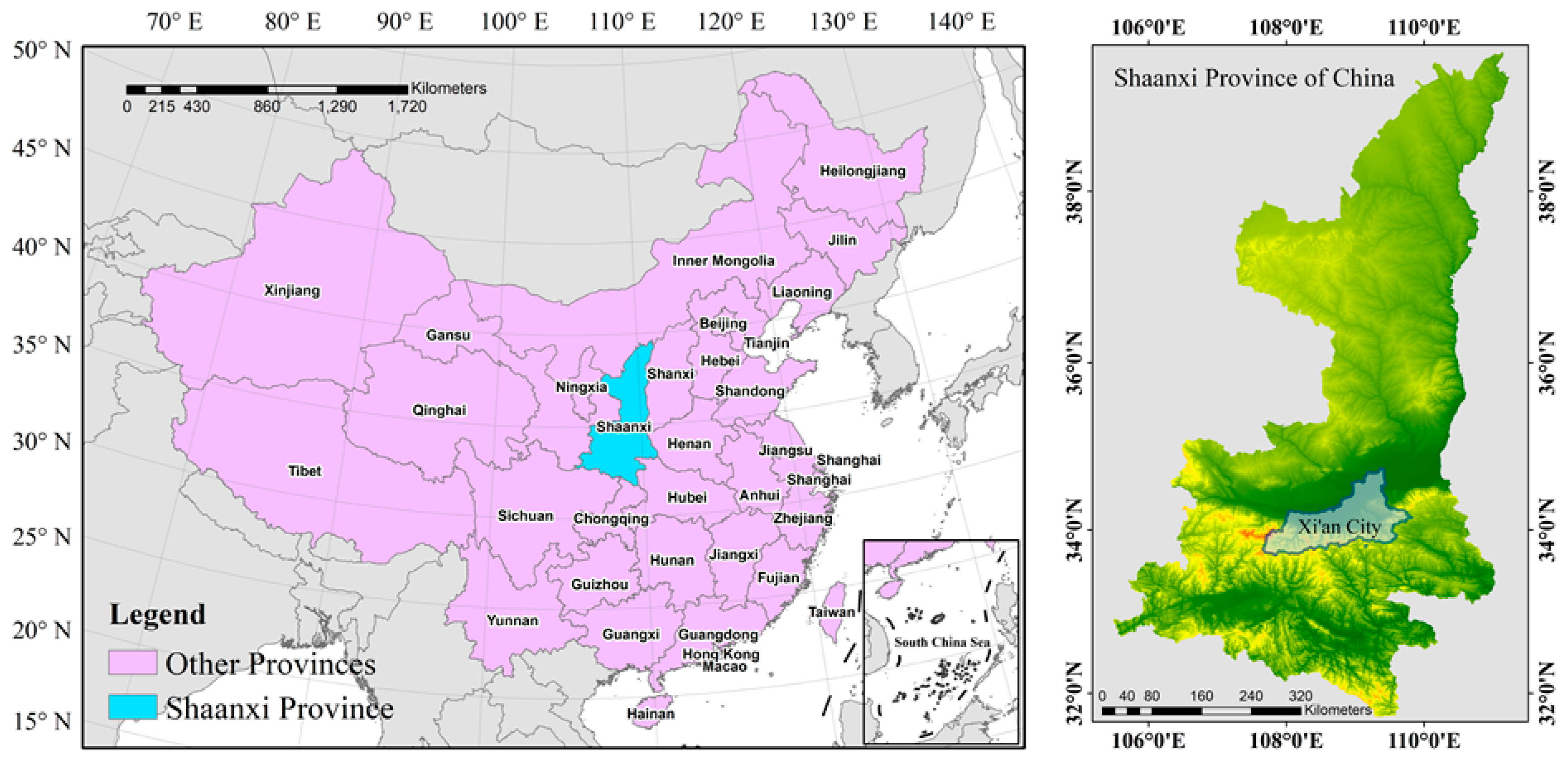
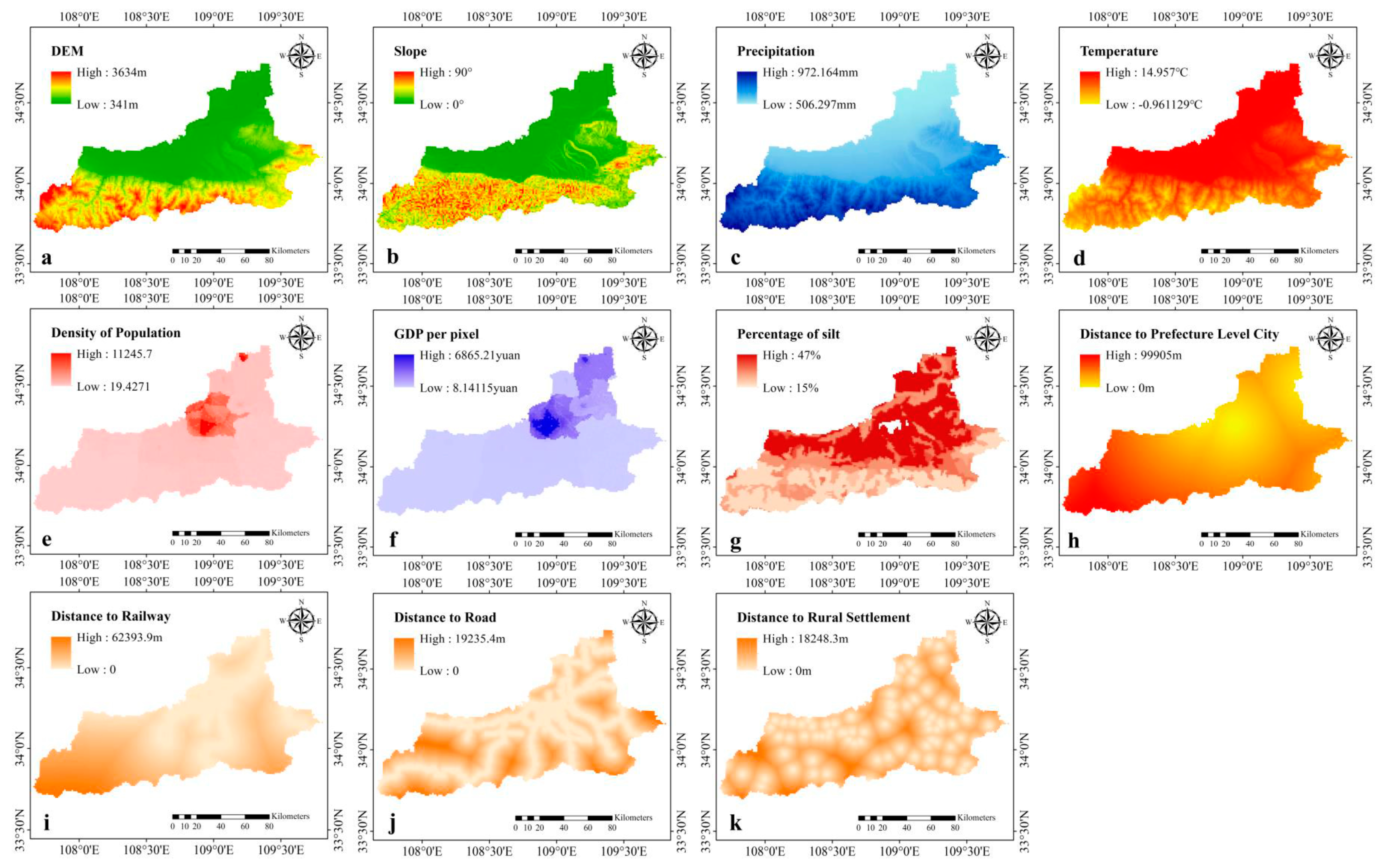
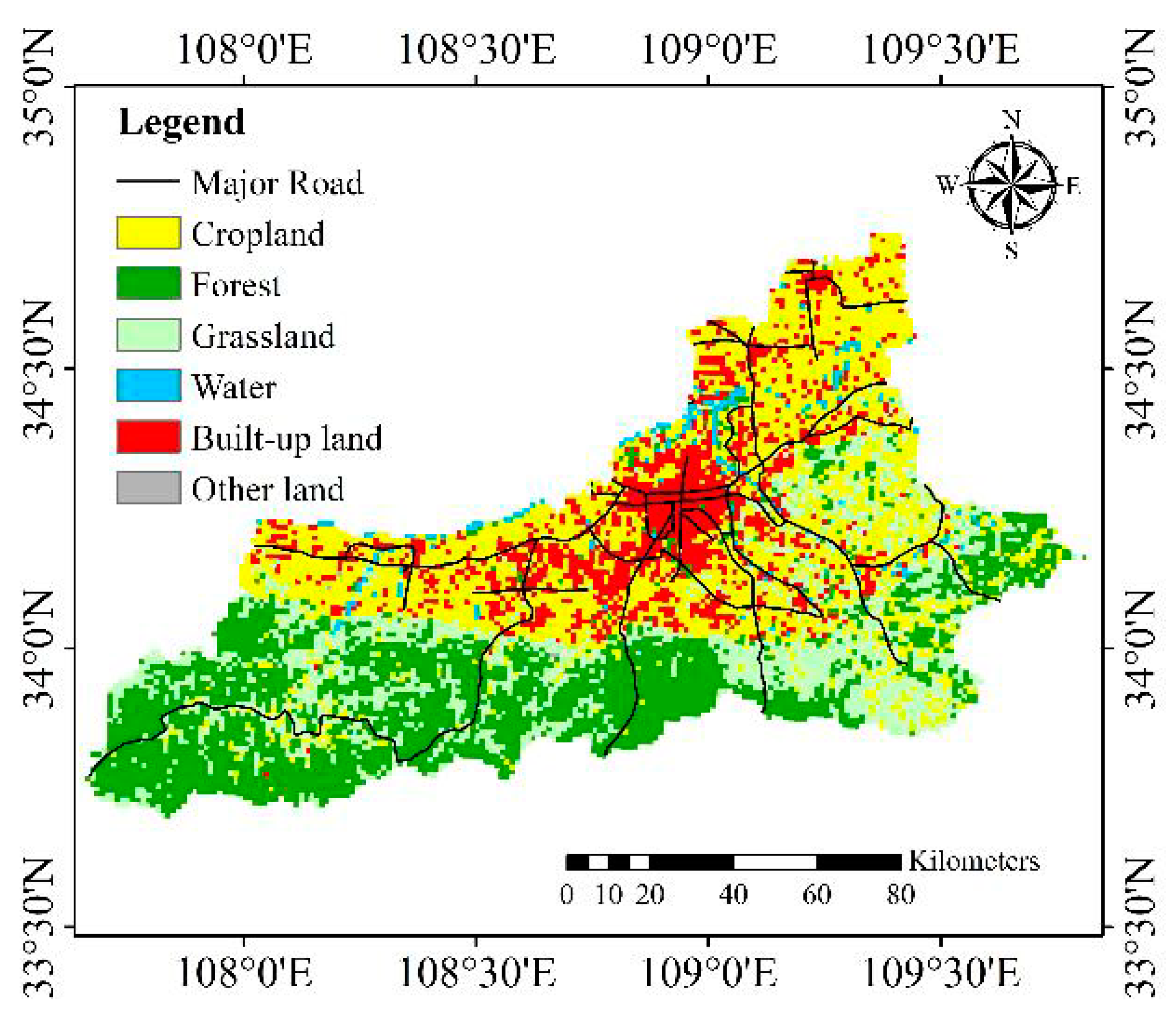
Xi’an city is located in the Loess Plateau region, which is one of the most well-known plateaus [46], and the Xi’an government has planned to construct a national central city aiming to not only develop the economy but also to drive the development of this Urban Agglomeration (http://www.shaanxi.gov.cn/zfgb/136373.htm (accessed on 3 January 2021). Xi’an is a prefecture-level city in China, which is the provincial capital, and the city is 204 km long from east to west and 116 km wide from north to south with a total area of 10108 square kilometers (Figure 1). It contains various terrains, such as mountains, hills, plains, and valleys, with an average altitude of 550 m. The average annual temperature and annual precipitation are 13.1 °C and 528.3–718.5 mm, respectively (http://www.xa.gov.cn/sq/csgk/zrdl/1.html (accessed on 3 January 2021)). The annual government revenue of Xi’an is 136.471 billion yuan, and the regional gross domestic product GDP was 746.985 billion yuan in 2018. The permanent resident population is 10.037 million and the newly built road area is 102.9172 million square meters. The selected influencing factors including biophysical and anthropogenic factors, are shown in Figure 2.
2.2. Data Source and Processing
Land use datasets (1990, 2000, and 2015) were provided by the Resource and Environment Data Cloud Platform, Institute of Geographic and Natural Resources Research, Chinese Academy of Sciences (CAS) (http://www.resdc.cn/ (accessed on 5 September 2020)). Furthermore, a description of the dataset is provided in Table 1.
Some datasets are updated to 2020, but it is necessary and important to ensure that all data pertain to the same year and are accessible. Moreover, some of the optional datasets are not allowed to download in certain years. Land use dataset is the primary datasets in our study, thus, we should firstly consider its temporal, spatial resolution, and accessibility. Resource and Environment Data Cloud Platform provides accessible and free land use data in 1990, 1995, 2000, 2005, 2010, 2015, 2018, and 2020. Nevertheless, the platform only provides relevant factor data up to 2015, such as precipitation and temperature. Therefore, considering the availability of the land use, anthropogenic factor, and biophysical factor datasets, we choose 2000 and 2015 as the model years. Relevant details of the biophysical and anthropogenic factors are listed in Table 2.
2.3. Methodology
In the study, the Markov model was adopted to predict the land use demand under future scenarios. Based on the land use quantity, the FLUS model was applied to simulate spatial land use change. Then, the complex network method was employed to analyze the land use systems and identify the key land use types during the different periods and future scenarios. Based on present and future land use scenarios, we analyzed the characteristics of land use change via different methods. The investigative framework is shown in Figure 3.
2.4. Methods
2.4.1. Markov-FLUS Model
The process of land use change simulation comprises two modules: a land use demand module to predict the future land use demand (Markov chain) and a spatial variation module to allocate the FLUS model. The Markov chain model is a stochastic method to describe the land demand with a transition probability matrix in land use change analysis [47]. The Markov chain model conveniently simulates changes that are difficult to describe [33]. Therefore, we selected the Markov chain model to assess the future land use demand. The transition probability between two different stages of land use was calculated to predict the future land use demand. The FLUS model is a combined model consisting of the system dynamic and CA models to model future land use patterns. The FLUS model attains a higher simulation accuracy than that of other land use change simulation models such as CLUE-S and CA [34]. Test result comparison has indicated that the overall accuracy and kappa coefficient of the FLUS model are indeed higher than those of the CLUE-S model. The simulation accuracy, e.g., the kappa coefficient, is an important criterion when choosing a model [34]. Obviously, it is more appropriate to apply the FLUS model to model land use patterns. In the FLUS model, the artificial neural network (ANs) technique is applied to calculate the probability of occurrence in each pixel. Furthermore, the conversion processes of the different land use types are commonly influenced by the conversion cost of land use pairs and the neighborhood weights of the individual land use types in land use units (pixels) during simulation.
2.4.2. Land Use Simulation Setting and Simulation Accuracy
The restricted area was defined as the region where land use change could not occur during land use simulation. In the restricted area, the FLUS model did not allow pixel change. Water was the main protective region to guarantee ecological security. Therefore, the water area was defined as the restricted area in our study, which indicates that the restricted area did not change during the simulation process. The neighborhood weights characterized the expansion of the different land use types. If the neighborhood weight approached 1, the land use type exhibited a notable expansion ability. If the neighborhood weight approached 0, the land use type exhibited a poor expansion ability. The different land use types attained varying neighborhood weights across different regions. In our study area, Xi’an city, the provincial capital of Shaanxi Province was selected, and city positioning accelerated the process of urbanization. Urban sprawl was the main driver of land use change. The “Grain for Green” program was implemented in 1999 and aimed to partially convert cropland into forest. Therefore, the neighborhood weights were set as follows: cropland: 0.1; forest: 0.2; grassland: 0.1; water: 0; built-up land: 1; and other land: 0.1.
The kappa coefficient reflects the model consistency between the simulated land use result and the true land use distribution [48]. A high kappa coefficient indicates a high simulation accuracy. When the kappa coefficient was lower than 0.8, we adjusted the original factors (Figure 2), reforecast the land use demand, and assessed the modelling parameters. The above procedure was repeated until the accuracy requirements were met (as shown in Figure 3). The equation is expressed as follows [49]:
where p0 and pe are the observed and expected fractions, respectively, of the land use.
2.4.3. Complex Network Model
The land use types were regarded as the nodes of the network, and the edges of the network represented the land use conversion process. The quantity of land use conversion was considered as the weight of the complex network model. The weighted indegree and weighted outdegree indicated the amount of land use transferred in and out of the area, respectively. Previous studies have only analyzed the characteristics of land use change, but few studies have focused on the characteristics of the total system in regard to land use change. The complex network model has previously been applied to analyze the characteristics of land use change in open-pit mining areas [50]. In our study, we selected the abovementioned model to investigate future land use changes including urban sprawl, via Gephi 0.9.2.
(1) Betweenness centrality
After the establishment of the land use system based on the complex network model, we calculated the various indicators of the land use system with Gephi 0.9.2. The betweenness centrality is defined as the number of nodes representing the shortest distance between two nodes [51]. The betweenness centrality was considered to characterize the influence of the nodes in the complex network model, which reflects the importance of the land use types in our study. High values of the betweenness centrality indicate more important land use types in the complex network model. Our study aimed to identify the key land use types during the different periods of land use change. The equation is expressed as follows:
where, Cb(i) is the value of the betweenness centrality, and gjk(i) and gjk denote the number of shortest paths between nodes j and k and the number of shortest paths connecting nodes i and k, respectively [51].
(2) Average shortest path length
In the same way, the average shortest path length, an indicator of the land use characteristics, was also calculated in Gephi 0.9.2. The average shortest path length was determined to character the efficiency of transmission in the complex network model. The average shortest path length assesses the stability of land use systems in the complex network model. The equation is expressed as follows [52]:
where dij is the edge between nodes i and j, and n is the number of land use types.
2.4.4. Characteristics of the land use
(1) Urban expansion index
The urban expansion index (UEI) was considered to evaluate the urbanization speed and is an improved technique based on the urbanization intensity index [53]. The UEI was determined to characterize the urbanization speed during the different land use simulation periods. This approach directly visualizes the urbanization process. The equation is expressed as follows:
where SUi+n and SUi are the urban areas at times i+n and i, respectively. S is the total study area, and n is the interval between the different times [53].
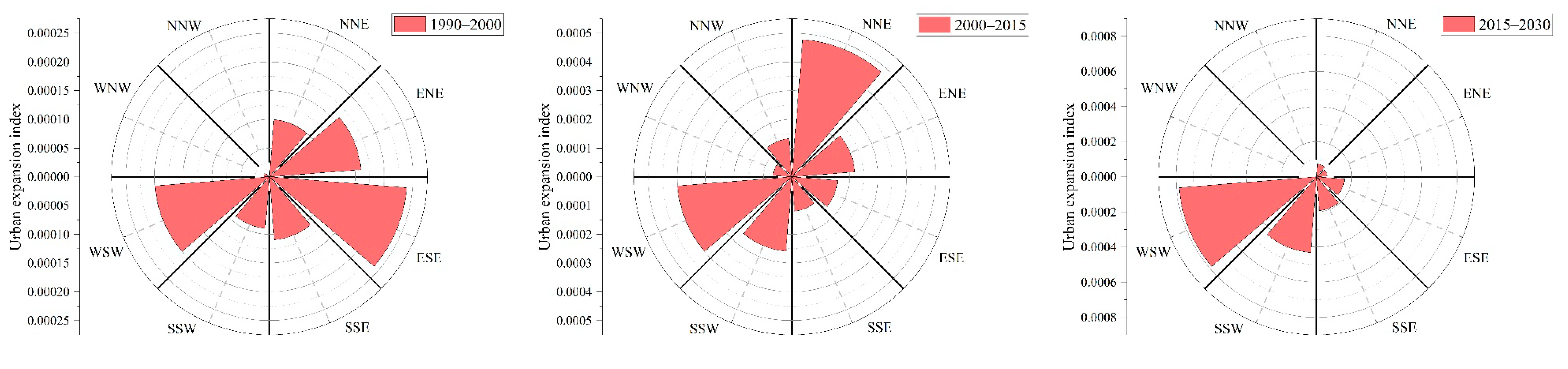
Xi’an was divided into eight directions to investigate the characteristics of urban expansion including north-northeast (NNE), east-northeast (ENE), east-southeast (ESE), south-southeast (SSE), south-southwest (SSW), west-southwest (WSW), west-northwest (WNW), and north-northwest (NNW).
(2) Gravity center model
The gravity center model aims to reveal the center of built-up land. It captures the characteristics of urban development over time. Our study aimed to analyze the features of land use changes. It was therefore necessary to investigate the gravity center of built-up land, which clearly reflected the gravity center of urban development and human activities. The gravity center clearly and quantitatively indicated the direction of urban sprawl. In this study, the gravity center was calculated during the different periods to characterize the spatial variation in urbanization. The formula equation was applied:
where, xi and yi are the coordinates of the ith pixel on the x and y axes, respectively, and xg and yg are the coordinates of the gravity center of built-up land.
where, D is the movement distance of the gravity center. xi and yi are the distance of movement in x axis and y axis, respectively.
(3) Land use pattern analysis
Fragstats 4.2 was used to analyze the land use pattern in the different years. The landscape pattern directly reflects the spatial characteristics of a given land use pattern. We investigated the land use pattern in two aspects including the class and landscape. Based on our study, we selected five class indicators and eight landscape indicators of the land use patterns (Table 3).
The selected land use patterns indicators highlighted the characteristics of land use change, which revealed different information on the various land use and land cover change (LUCC) patterns. Moreover, the landscape and class indicators reflected the characteristics of the total study area and the different land use types, respectively, in our research. Furthermore, we selected a few indicators to comprehensively reveal the land use patterns, including urban sprawl. Hence, certain indicators have similar meanings. Therefore, we selected the abovementioned indicators (landscape and class) based on the relevant definitions contained in official instructions. The definitions of the indicators are listed in Table 4 (McGarigal, K., SA Cushman, and E Ene. 2012. FRAGSTATS v4: Spatial Pattern Analysis Program for Categorical and Continuous Maps. Computer software program produced by the authors at the University of Massachusetts, Amherst.).
3. Results
3.1. Accuracy Evaluation of the Simulations
The accuracy of the land use change simulations is summarized in Table 5. The kappa coefficient of the FLUS model was 0.922535. The producer accuracy was higher than 0.7 for the different land use types. Moreover, the user accuracy was higher than 0.9 for all land use types. It was concluded that the accuracy (2000–2015) met the land use change simulation requirements. Therefore, the set parameters, such as the selected factors and neighborhood weights, satisfied the accuracy requirements.
3.2. General Land Use Change and Simulation
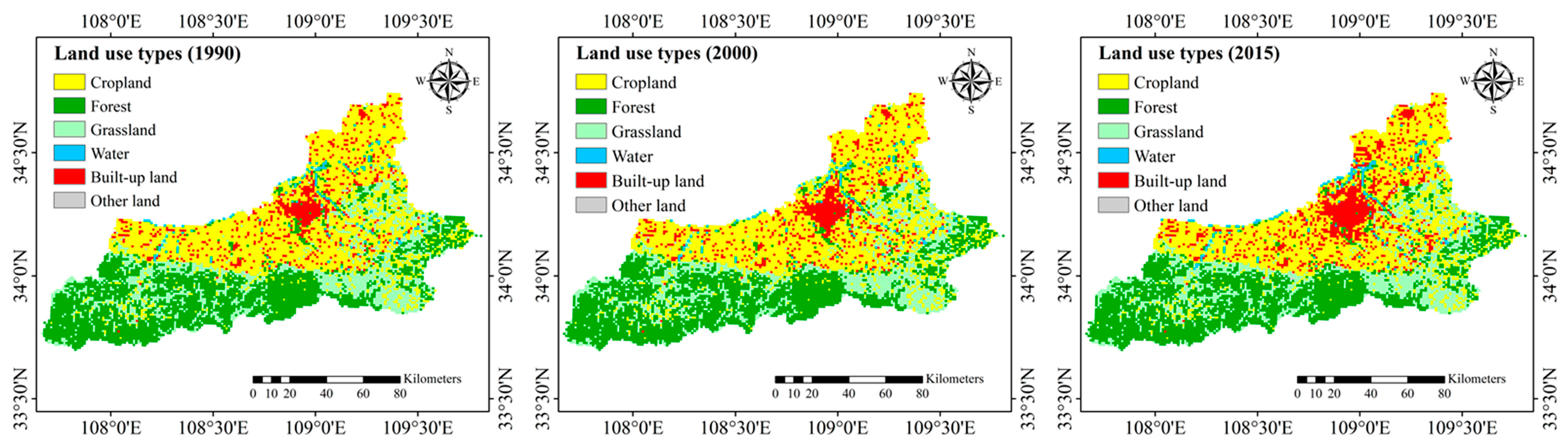
Figure 4 shows the obvious land use change in recent years. As shown in Figure 5, the simulation results of the land use change demonstrated dramatic changes from 2015 to 2030. Built-up land experienced obviously continuous expansion from 2015–2030, and it was concluded that urbanization remained the primary land use change direction in the future. Detailed land use change dynamics are shown in Figure 6. Dramatic land use change occurred from 1990–2000. The various processes of land use change were mainly distributed along the built-up land boundary from 2000–2015 and 2015–2030. Nevertheless, the processes exhibited no obvious change in the natural land use type such as forest, grassland, and water over the 1990–2000 period.
3.3. Analysis of the Characteristics of Land Use Change
3.3.1. Land Use Characteristics
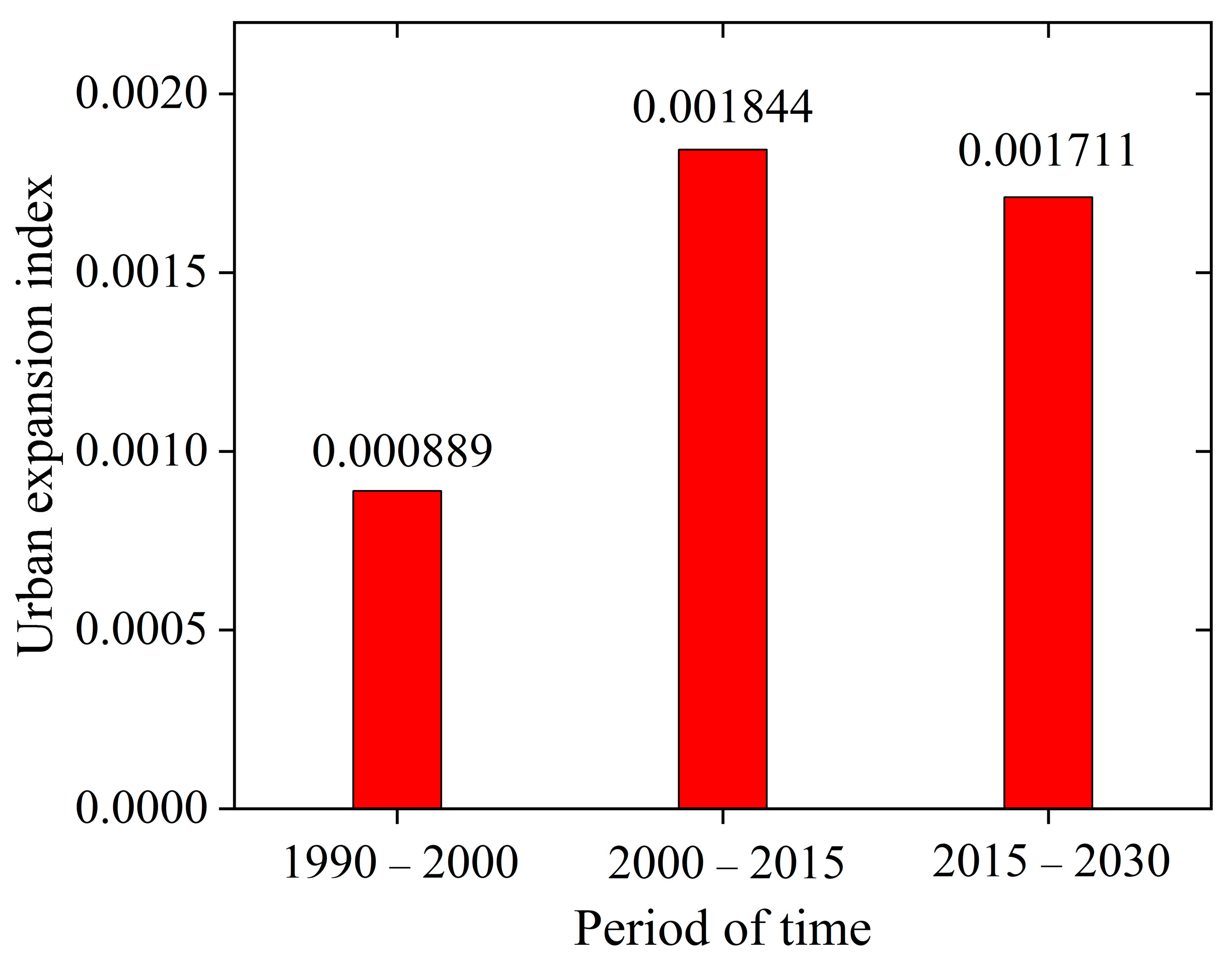
The trajectory of the gravity center is shown in Figure 7. The gravity center moved to the east and then to the southwest in the next stage. During the period from 1990 to 2015, no movement was observed in the gravity center. Nevertheless, the gravity center moved 1 and 2.828 km from 2000–2015 and 2015–2030, respectively. The UEI is shown in Figure 8. The UEI reflected the urbanization speed over time. From 1990 to 2015, urban expansion first increased and then decreased. The UEI reached values of 0.000889, 0.001844 and 0.001711 during the period from 1990–2000, 2000–2015 and 2015–2030, respectively. As shown in Figure 9, the primary urban development directions were ESE, NNE, and WSW during the periods from 1990–2000, 2000–2015 and 2015–2030, respectively. In particular, the urban expansion magnitude along the major directions during the different periods also gradually increased over time.
3.3.2. Land Pattern Characteristics
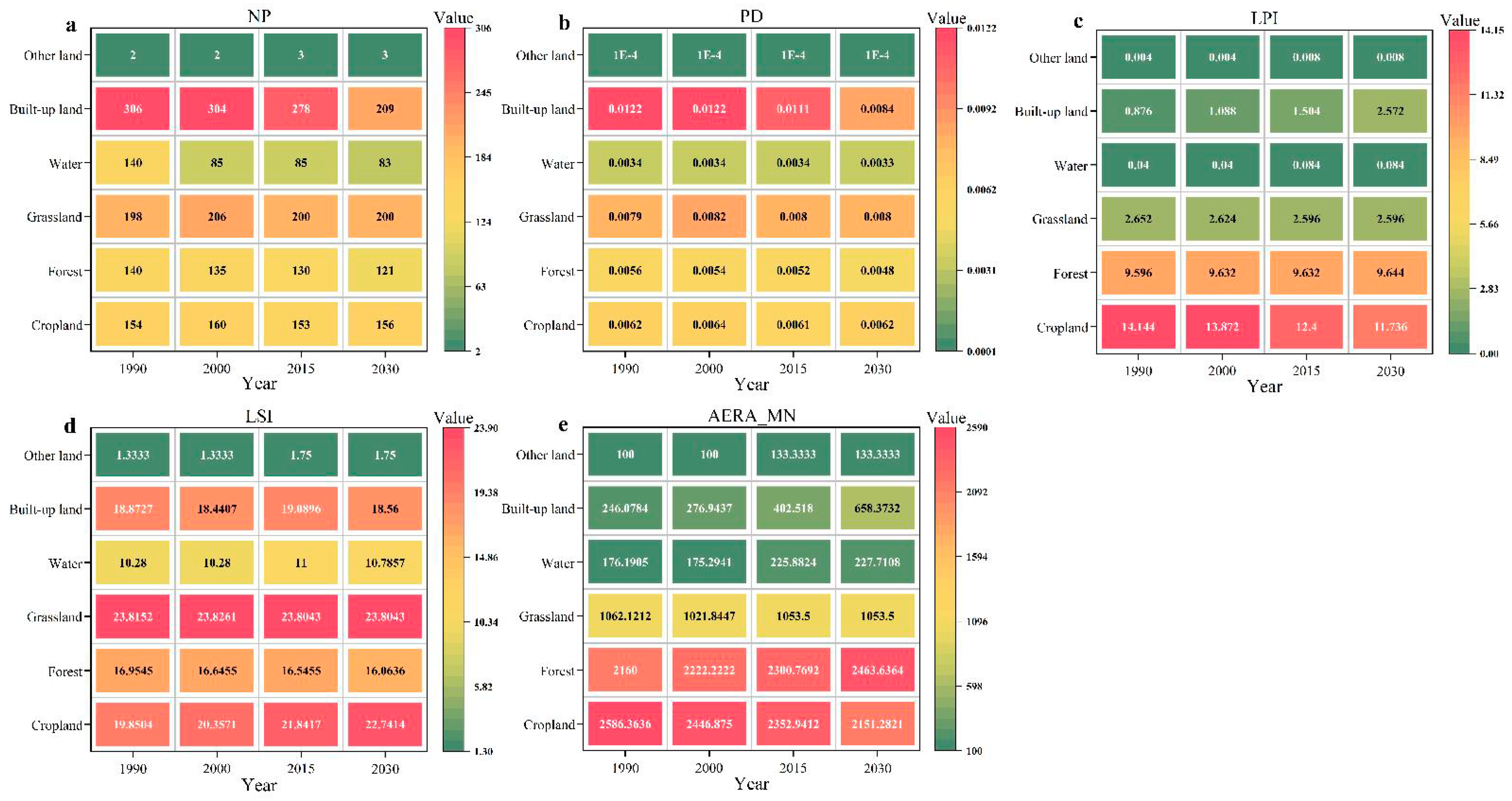
The land use patterns of the different land use types are shown in Figure 10. Compared to the other land use types, the number of patches (NP) of the built-up land and water exhibited a dramatic decrease. The patch density (PD) of built-up land also demonstrated an obviously negative change. The largest patch index (LPI) of cropland and built-up land revealed that the largest patch areas of these land use types obviously decreased. Nevertheless, the landscape shape index (LSI) indicated a relatively stable change during the study period. The mean patch size (AREA_MN) of all land use types demonstrated obvious changes from 1990 to 2030, especially in regard to the built-up land and cropland areas. The average built-up land and cropland areas increased and decreased, respectively.
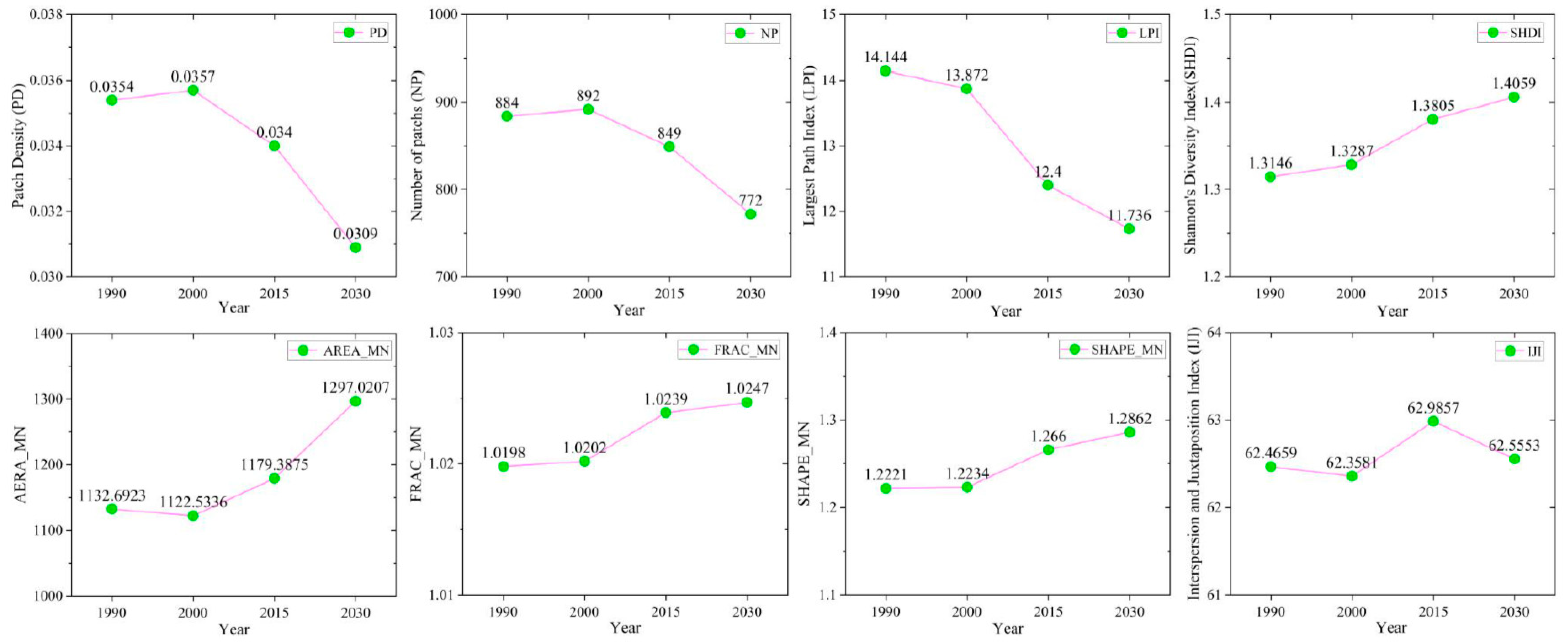
The LPI revealed a continuous decrease during the study period (Figure 11). However, Shannon’s diversity index (SHDI), mean patch area (AREA_MN), perimeter-area fractal dimension (FRAC_MN), and mean patch shape index (SHAPE_MN) demonstrated a continuous increase. In contrast, the PD, NP, and interspersion and juxtaposition index (IJI) fluctuated.
3.4. Characteristics of the Land Use Change Network
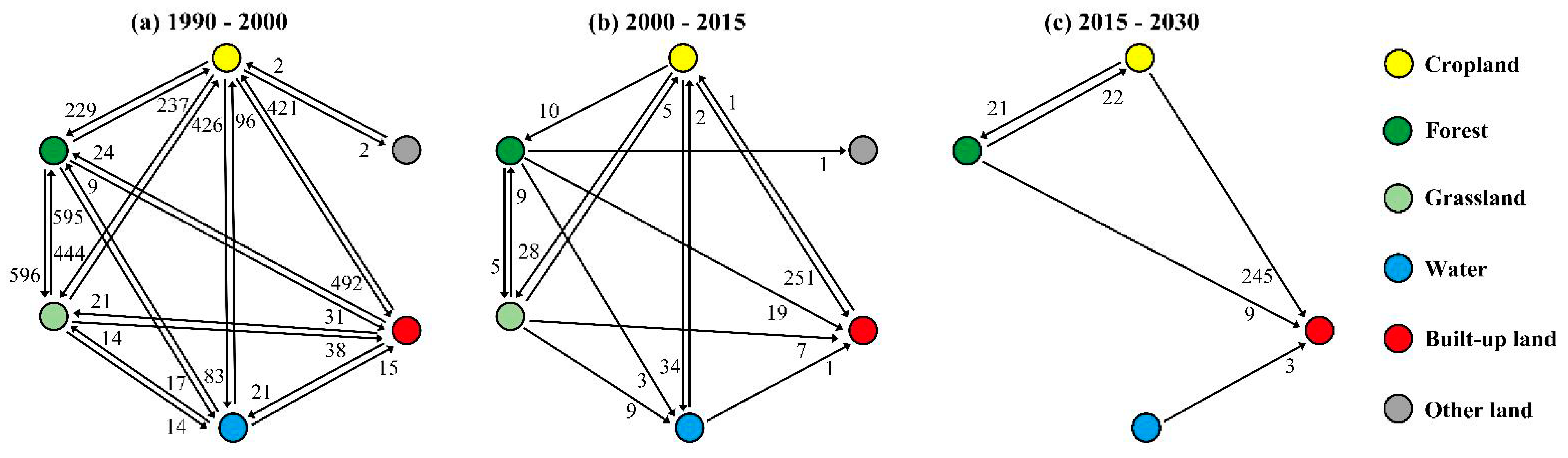
Complex networks of the land use cover change from 1990–2000, 2000–2015, and 2015–2030) are shown in Figure 12a–c, respectively. The nodes played different roles among the edges and nodes based on the weights. All land use types experienced land conversion in the network from 1990–2000. High-weight conversion mainly occurred from cropland into forest, cropland into grassland, cropland into water, cropland into built-up land, and forest into built-up land during the period from 2000–2015. High-weight conversion was mostly observed in the relationships of cropland with forest, cropland with built-up land, and forest with cropland during the period from 2015–2030.
If the weighted indegree was higher than the weighted outdegree, the observed land use type was input land. Otherwise, output land was indicated. The weighted indegree and weighted outdegree from 1990–2000, 2000–2015 and 2015–2030 are listed in Table 6, Table 7 and Table 8, respectively. During the period from 2000 to 2015, the input land included grassland, water, built-up land, and other land, and the output land included cropland and forest. During the period of 2015–2030, built-up land contributed to the input land, while cropland, forest, and water contributed to the output land.
The betweenness centrality of the land use change was 8.0 for cropland from 1990 to 2000 (Table 9). During the period from 2000 to 2015, the betweenness centrality greatly differed among the various land use types (Table 10). The betweenness centrality values for cropland, forest, grassland, water, built-up land, and other land were 7.0, 1.5, 1.83, 0.33, 0.33, and 0.0, respectively. Nevertheless, all land use types attained a betweenness centrality value of 0 between 2015 and 2030 (Table 11). Cropland was the key land use type in the observed land use change from 1990–2000 and 2000–2015.
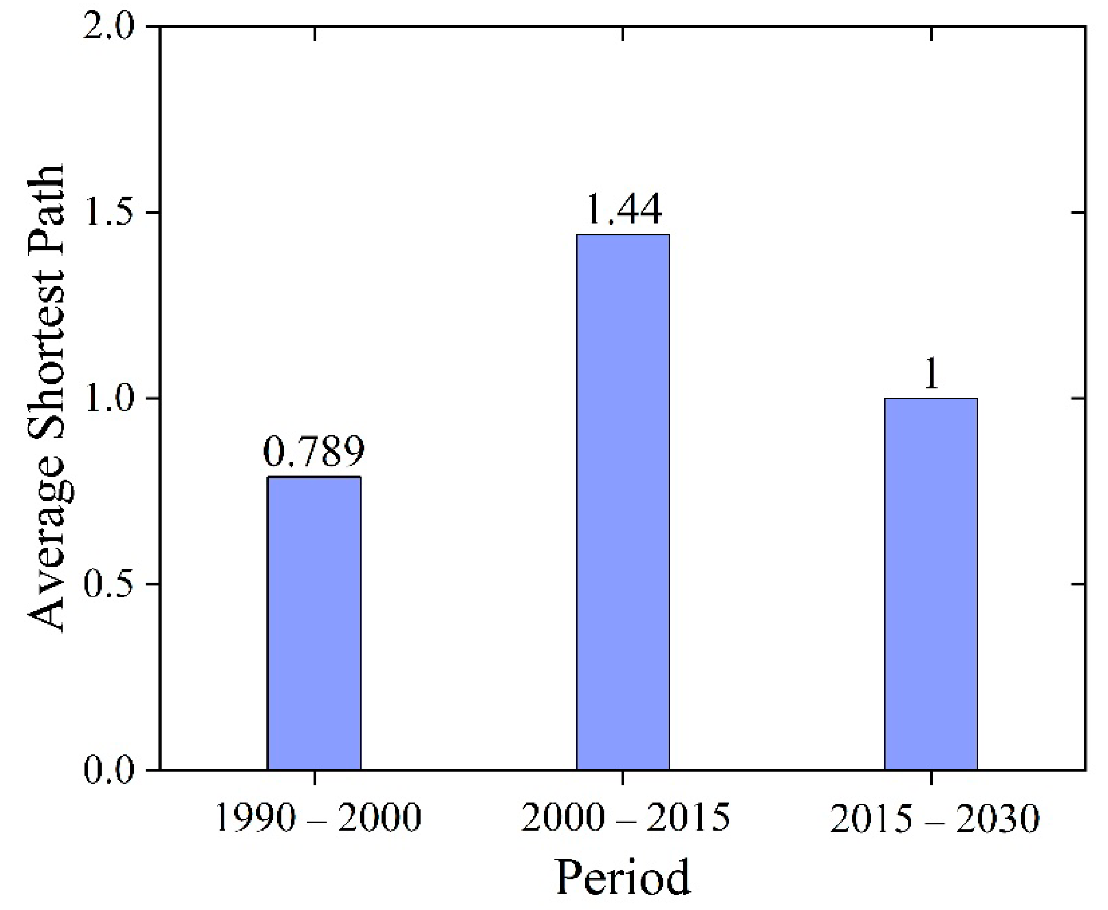
The values of the average shortest paths were 0.789, 1.44, and 1 (Figure 13). The average shortest path during the period from 2000–2015 was larger than that during the period from 2015–2030. This demonstrated that the stability of the land use system decreased during the next period.
4. Discussion
4.1. Urban Development and Ecological Environment
The simulations revealed that urban sprawl dramatically altered the land use pattern. Anthropogenic activities indeed influenced land use change and altered the ecological environment [3]. In Xi’an, as the provincial capital, an increasing number of people strove to attain personal or family development. Hence, the demand of built-up land increased with the population density. This accelerated urban sprawl and necessitated the government to implement land expropriation [54]. In our simulation results, urban sprawl continuously increased, and cropland was converted into built-up land. This indicated large-scale expansion at the current development speed. Our urban expansion characteristics were similar to those reported by Yang et al. [55] in the Beijing-Tianjin-Hebei region. Land use patterns changed, which was driven by urban expansion and cropland loss. Furthermore, the results indicated that the UEI presented a decreasing trend during the period from 2015–2030 over the period from 2000–2015. Nevertheless, the index values during the 2000–2015 and 2015–2030 periods were still obviously higher than those during the 1990–2000 period, which indicated that urban expansion remained high in the future. Moreover, the future gravity center of urban development moved approximately along the opposite direction in the current simulations. The resistance to development seemed to be lower in the southwest than that in the northeast. ESE, NNE, and WSW were the major urban expansion directions during the different periods. In fact, urban expansion typically faces a trade-off between rapid urban expansion and the ecological environment. Continuous and rapid urban sprawl experiences three main challenges, i.e., the loss of high-quality cropland, overdevelopment of cities to form hollow cities, and ecological environmental effects [56]. However, compared to the 1990–2000 period, the stability of the land system obviously increased during the 2000–2015 period. Compared to the period from 2000–2015, the stability of the land system revealed a decreasing trend from 2015–2030. Therefore, the government should continue to pursue not only urban development but also urban ecological environment maintenance. Although the area of the urban region is limited, urban planners should improve the land use efficiency such as the reuse of urban abandoned land and reconstruction of old towns, instead of simply requisitioning cropland to develop urban borders areas. A decrease in cropland may impose a major influence on food security, and urbanization may also affect the local air quality [57]. Therefore, the government should carefully consider urbanization.
4.2. “Grain for Green” Program
The “Grain for Green” program was implemented in 1999 [58]. Network conversion gradually simplified during the above three periods, i.e., 1990–2000, 2000–2015 and 2015–2030. The land use changed from 2000–2015. The “Grain for Green” program required very high government financial investment to compensate for the economic loss of farmers. Moreover, the program aimed to protect the ecological environment and prevent soil erosion in high-slope cropland regions. Indeed, previous studies have reported that the “Grain for Green” program contributed more than 20% to the large-scale increase in vegetation cover on the Loess Plateau [59], which is similar to our greening results (conversion into forest, cropland, and grassland). The results from 2000–2015 showed that several cropland areas were converted into forest and grassland. It was further revealed that a decrease in land system stability occurred. A related study has reported that “the planting of inappropriate species and an overemphasis on trees and shrubs compromise the ability to achieve environmental policy goals”[60]. The “Grain for Green” program must also consider the comprehensive effects between afforestation and the local environment. Otherwise, an unstable land use system may be established. Natural land use types should be a focus of increasing attention in land reclamation and consolidation. The “Grain for Green” program aimed to protect the natural environment and has yielded no seriously negative effects on grain security [61]; nevertheless, grain security has remained a vital goal in China. Therefore, the partial conflicts between the ecological environment and agricultural production should be continuously addressed in the future.
4.3. Cropland Protection and Efficient Utilization
Cropland areas exhibited a continuous decrease during the three periods, which was mainly driven by urbanization [62,63]. Cropland attained the highest betweenness centrality value during the periods from 1990–2000 and 2000–2015. It was concluded that cropland played an important role in the total land use change. Related research on open-pit mining areas has reported that “cropland is the key land use type during the periods from 1986–2009, 2009–2013, and 2013–2015” [50]. Similarly, cropland played a key role in the land use system. Therefore, cropland should be given more attention such as protection and efficient utilization. In fact, the government has implemented the related policies to protect cropland and improve the efficiency of land use, which is part of the reason for the highest value of betweenness centrality of cropland in land use systems [64]. Although the areas of cropland decreased, cropland production still continuously increased due to agricultural intensification. Nevertheless, this does not indicate that we should occupy cropland without limits. Moreover, we should further strengthen cropland protection. Cropland reclamation is a large project requiring high government investment and much time to repair the cultivation layer and restore the ability to grow crops. In particular, unutilized and inefficient land areas should be assessed and integrated into existing farmland areas as much as possible, thus giving full play to the benefits of agricultural scale. Cropland must remain protected in general land use planning, and the cropland area should be gradually increased in over time.
5. Policies Implication
5.1. Continuously Implemented Afforestation
Under future scenarios, the forest area will increase continuously and extensively. Nevertheless, forest loss still occurs, which results in fragmentation driven by anthropogenic factors [65]. Regarding local governments, new ecological policies should be implemented continuously and existing forest regions should be protected. The conflict between ecological protection and economic development has always been an important trade-off process at the local scale. At all levels, the government must also protect the original forest as much as possible in addition to the promotion of afforestation in the Loess Plateau region. Afforestation should continuously focus on fragile areas, such as high-gradients areas and land degradation regions. Moreover, continuously implemented afforestation measures should focus more on trees adapted to local climate and environmental conditions [60]. This enables afforestation policies to more positively influence fragile areas, such as the Loess Plateau region. Finally, forest protection must continue after planting.
5.2. Scientific Control of Rapid Urban Expansion and Cropland Protection
Urban expansion exhibits a continuous increase, and cropland decreases under future scenarios. Urbanization encroaches cropland to destroy the original ecosystem. Nevertheless, cropland is a fundamental guarantee for food security. It is necessary to protect cropland and control rapid urban expansion. The process of pursuing economic development must choose effectiveness over quantity. In the future, local governments (prefecture-level cities) should increase the land use intensity and stop unscientific urban expansion. In particular, policy-makers at all levels should focus on the inefficient use of built-up and abandoned urban land areas. The public often ignores the developmental capacity of abandoned urban land. The trade-off between urban expansion and cropland protection will remain a key concern.
5.3. Effective Redevelopment of Un-Utilized Land
Abandoned land has gradually increased, and the effectiveness of land use is extremely low. The government should pay attention to the redevelopment of unused land in the future. It is important to encourage public legal redevelopment of unused land via the establishment of motivating mechanisms. The local government, including prefecture- and county-level cities, should lead to the redevelopment process of unutilized land.
6. Conclusions
Our study simulated future land use situation with the Markov and FLUS models, and analyzed the spatiotemporal land use change via the UEI, gravity model, and land use pattern analyses in Xi’an city. Based on the complex network model, we identified the key land use type and calculated the stability of the land use system during different periods. According to our modelling results, built-up land exhibited a continuous increase. Nevertheless, cropland obviously revealed the opposite trend in the future, namely, a decreasing trend. The gravity center moved eastward and southwestward during the period from 2000–2015 and 2015–2030, respectively. The urban expansion speed first increased and then decreased, and a high expansion level was sustained. The primary urban development directions were ESE, NNE, and WSW during the 1990–2000, 2000–2015 and 2015–2030 periods, respectively. Cropland played a key role in land use dynamics from 1990–2000 and 2000–2015. The land use system stability will decrease in the future, which indicates potential instability issues in future land use change. The ecological environment should be further considered and researched in the future.
Author Contributions
Conceptualization, D.F. and W.B.; methodology, D.F., W.B., M.F. and Y.S.; software, D.F. and W.B.; formal analysis, D.F. and M.Z.; investigation, D.F. and W.B.; data curation, D.F. and W.B.; Writing—Original draft preparation, D.F., M.Z. and Y.S.; Writing—Review and editing, D.F. and M.F.; visualization, D.F. and M.Z.; project administration, M.F.; funding acquisition, M.F. All authors have read and agreed to the published version of the manuscript.
Funding
This research was funded by the National Natural Science Foundation of China, grant number 41771204 and The APC was funded by Meichen Fu.
Data Availability Statement
Not applicable.
Conflicts of Interest
The authors declare no conflict of interest.
References
- Sterling, S.M.; Ducharne, A.; Polcher, J. The impact of global land-cover change on the terrestrial water cycle. Nat. Clim. Chang. 2012, 3, 385–390. [Google Scholar] [CrossRef]
- Tian, H.; Lu, C.; Ciais, P.; Michalak, A.M.; Canadell, J.G.; Saikawa, E.; Huntzinger, D.N.; Gurney, K.R.; Sitch, S.; Zhang, B.; et al. The terrestrial biosphere as a net source of greenhouse gases to the atmosphere. Nat. Cell Biol. 2016, 531, 225–228. [Google Scholar] [CrossRef] [PubMed] [Green Version]
- Song, X.-P.; Hansen, M.C.; Stehman, S.V.; Potapov, P.V.; Tyukavina, A.; Vermote, E.F.; Townshend, J.R. Global land change from 1982 to 2016. Nat. Cell Biol. 2018, 560, 639–643. [Google Scholar] [CrossRef] [PubMed]
- Poeplau, C.; Don, A.; Vesterdal, L.; Leifeld, J.; Van Wesemael, B.; Schumacher, J.; Gensior, A. Temporal dynamics of soil organic carbon after land-use change in the temperate zone—Carbon response functions as a model approach. Glob. Chang. Biol. 2011, 17, 2415–2427. [Google Scholar] [CrossRef]
- Seto, K.C.; Güneralp, B.; Hutyra, L.R. Global forecasts of urban expansion to 2030 and direct impacts on biodiversity and carbon pools. Proc. Natl. Acad. Sci. USA 2012, 109, 16083–16088. [Google Scholar] [CrossRef] [PubMed] [Green Version]
- Verburg, P.H.; Neumann, K.; Nol, L. Challenges in using land use and land cover data for global change studies. Glob. Chang. Biol. 2011, 17, 974–989. [Google Scholar] [CrossRef] [Green Version]
- Arias-Ortiz, A.; Serrano, O.; Masqué, P.; Lavery, P.S.; Mueller, U.; Kendrick, G.A.; Rozaimi, M.; Esteban, A.; Fourqurean, J.W.; Marbà, N.; et al. A marine heatwave drives massive losses from the world’s largest seagrass carbon stocks. Nat. Clim. Chang. 2018, 8, 338–344. [Google Scholar] [CrossRef] [Green Version]
- Wu, D.H.; Zhao, X.; Liang, S.L.; Zhou, T.; Huang, K.C.; Tang, B.J.; Zhao, W.Q. Time-lag effects of global vegetation responses to climate change. Glob. Chang. Biol. 2015, 21, 3520–3531. [Google Scholar] [CrossRef] [PubMed]
- Friend, A.D.; Lucht, W.; Rademacher, T.T.; Keribin, R.; Betts, R.; Cadule, P.; Ciais, P.; Clark, D.B.; Dankers, R.; Falloon, P.D.; et al. Carbon residence time dominates uncertainty in terrestrial vegetation responses to future climate and atmospheric CO2. Proc. Natl. Acad. Sci. USA 2014, 111, 3280–3285. [Google Scholar] [CrossRef] [Green Version]
- Yin, H.; Pflugmacher, D.; Li, A.; Li, Z.; Hostert, P. Land use and land cover change in Inner Mongolia—Understanding the effects of China’s re-vegetation programs. Remote Sens. Environ. 2018, 204, 918–930. [Google Scholar] [CrossRef]
- Christensen, P.; Mccord, G.C. Geographic determinants of China’s urbanization. Reg. Sci. Urban Econ. 2016, 59, 90–102. [Google Scholar] [CrossRef] [Green Version]
- Tong, X.; Wang, K.; Brandt, M.; Yue, Y.; Liao, C.; Fensholt, R. Assessing Future Vegetation Trends and Restoration Prospects in the Karst Regions of Southwest China. Remote Sens. 2016, 8, 357. [Google Scholar] [CrossRef] [Green Version]
- Ziadat, F.M.; Taimeh, A.Y. Effect of rainfall intensity, slope, land use and antecedent soil moisture on soil erosion in an arid environment. Land Degrad. Dev. 2013, 24, 582–590. [Google Scholar] [CrossRef]
- El Kateb, H.; Zhang, H.; Zhang, P.; Mosandl, R. Soil erosion and surface runoff on different vegetation covers and slope gradients: A field experiment in Southern Shaanxi Province, China. Catena 2013, 105, 1–10. [Google Scholar] [CrossRef]
- Shen, H.; Zheng, F.; Wen, L.; Han, Y.; Hu, W. Impacts of rainfall intensity and slope gradient on rill erosion processes at loessial hillslope. Soil Tillage Res. 2016, 155, 429–436. [Google Scholar] [CrossRef]
- Wei, Y.D.; Li, H.; Yue, W. Urban land expansion and regional inequality in transitional China. Landsc. Urban Plan. 2017, 163, 17–31. [Google Scholar] [CrossRef]
- Zheng, K.; Wei, J.-Z.; Pei, J.-Y.; Cheng, H.; Zhang, X.-L.; Huang, F.-Q.; Li, F.-M.; Ye, J.-S. Impacts of climate change and human activities on grassland vegetation variation in the Chinese Loess Plateau. Sci. Total. Environ. 2019, 660, 236–244. [Google Scholar] [CrossRef]
- Alexander, P.; Rounsevell, M.D.; Dislich, C.; Dodson, J.R.; Engström, K.; Moran, D. Drivers for global agricultural land use change: The nexus of diet, population, yield and bioenergy. Glob. Environ. Chang. 2015, 35, 138–147. [Google Scholar] [CrossRef] [Green Version]
- Dadashpoor, H.; Azizi, P.; Moghadasi, M. Land use change, urbanization, and change in landscape pattern in a metropolitan area. Sci. Total. Environ. 2019, 655, 707–719. [Google Scholar] [CrossRef] [PubMed]
- Tong, D.; Wang, X.; Wu, L.; Zhao, N. Land ownership and the likelihood of land development at the urban fringe: The case of Shenzhen, China. Habitat Int. 2018, 73, 43–52. [Google Scholar] [CrossRef]
- Wu, Y.; Luo, J.; Zhang, X.; Skitmore, M. Urban growth dilemmas and solutions in China: Looking forward to 2030. Habitat Int. 2016, 56, 42–51. [Google Scholar] [CrossRef] [Green Version]
- Freitas, S.R.; Hawbaker, T.J.; Metzger, J.P. Effects of roads, topography, and land use on forest cover dynamics in the Brazilian Atlantic Forest. For. Ecol. Manag. 2010, 259, 410–417. [Google Scholar] [CrossRef]
- Song, W. Decoupling cultivated land loss by construction occupation from economic growth in Beijing. Habitat Int. 2014, 43, 198–205. [Google Scholar] [CrossRef]
- Toth, C.; Jóźków, G. Remote sensing platforms and sensors: A survey. ISPRS J. Photogramm. Remote. Sens. 2016, 115, 22–36. [Google Scholar] [CrossRef]
- Atzberger, C. Advances in Remote Sensing of Agriculture: Context Description, Existing Operational Monitoring Systems and Major Information Needs. Remote Sens. 2013, 5, 949–981. [Google Scholar] [CrossRef] [Green Version]
- Hussain, M.; Chen, D.; Cheng, A.; Wei, H.; Stanley, D. Change detection from remotely sensed images: From pixel-based to object-based approaches. ISPRS J. Photogramm. Remote Sens. 2013, 80, 91–106. [Google Scholar] [CrossRef]
- Dewan, A.M.; Yamaguchi, Y. Land use and land cover change in Greater Dhaka, Bangladesh: Using remote sensing to promote sustainable urbanization. Appl. Geogr. 2009, 29, 390–401. [Google Scholar] [CrossRef]
- Ning, J.; Liu, J.; Kuang, W.; Xu, X.; Zhang, S.; Yan, C.; Li, R.; Wu, S.; Hu, Y.; Du, G.; et al. Spatiotemporal patterns and characteristics of land-use change in China during 2010–2015. J. Geogr. Sci. 2018, 28, 547–562. [Google Scholar] [CrossRef] [Green Version]
- Mustafa, A.; Heppenstall, A.; Omrani, H.; Saadi, I.; Cools, M.; Teller, J. Modelling built-up expansion and densification with multinomial logistic regression, cellular automata and genetic algorithm. Comput. Environ. Urban Syst. 2018, 67, 147–156. [Google Scholar] [CrossRef] [Green Version]
- Shen, Q.; Chen, Q.; Tang, B.-S.; Yeung, S.; Hu, Y.; Cheung, G. A system dynamics model for the sustainable land use planning and development. Habitat Int. 2009, 33, 15–25. [Google Scholar] [CrossRef]
- Lin, J.; Gau, C. A TOD planning model to review the regulation of allowable development densities around subway stations. Land Use Policy 2006, 23, 353–360. [Google Scholar] [CrossRef]
- Halmy, M.W.A.; Gessler, P.E.; Hicke, J.A.; Salem, B.B. Land use/land cover change detection and prediction in the north-western coastal desert of Egypt using Markov-CA. Appl. Geogr. 2015, 63, 101–112. [Google Scholar] [CrossRef]
- Yang, X.; Zheng, X.-Q.; Lv, L.-N. A spatiotemporal model of land use change based on ant colony optimization, Markov chain and cellular automata. Ecol. Model. 2012, 233, 11–19. [Google Scholar] [CrossRef]
- Liu, X.; Liang, X.; Li, X.; Xu, X.; Ou, J.; Chen, Y.; Li, S.; Wang, S.; Pei, F. A future land use simulation model (FLUS) for simulating multiple land use scenarios by coupling human and natural effects. Landsc. Urban Plan. 2017, 168, 94–116. [Google Scholar] [CrossRef]
- Zheng, F.; Hu, Y. Assessing temporal-spatial land use simulation effects with CLUE-S and Markov-CA models in Beijing. Environ. Sci. Pollut. Res. 2018, 25, 32231–32245. [Google Scholar] [CrossRef] [PubMed]
- Zhou, R.; Zhang, H.; Ye, X.-Y.; Wang, X.-J.; Su, H.-L. The Delimitation of Urban Growth Boundaries Using the CLUE-S Land-Use Change Model: Study on Xinzhuang Town, Changshu City, China. Sustainability 2016, 8, 1182. [Google Scholar] [CrossRef] [Green Version]
- Zhang, D.; Liu, X.; Lin, Z.; Zhang, X.; Zhang, H. The delineation of urban growth boundaries in complex ecological environment areas by using cellular automata and a dual-environmental evaluation. J. Clean. Prod. 2020, 256, 120361. [Google Scholar] [CrossRef]
- Fox, J.; Vogler, J.B.; Sen, O.L.; Giambelluca, T.W.; Ziegler, A.D. Simulating Land-Cover Change in Montane Mainland Southeast Asia. Environ. Manag. 2012, 49, 968–979. [Google Scholar] [CrossRef] [PubMed]
- Xia, T.; Wu, W.; Zhou, Q.; Verburg, P.H.; Yu, Q.; Yang, P.; Ye, L. Model-based analysis of spatio-temporal changes in land use in Northeast China. J. Geogr. Sci. 2015, 26, 171–187. [Google Scholar] [CrossRef]
- Zheng, X.-Q.; Zhao, L.; Xiang, W.-N.; Li, N.; Lv, L.-N.; Yang, X. A coupled model for simulating spatio-temporal dynamics of land-use change: A case study in Changqing, Jinan, China. Landsc. Urban Plan. 2012, 106, 51–61. [Google Scholar] [CrossRef]
- Du, X.; Zhao, X.; Liang, S.; Zhao, J.; Xu, P.; Wu, D. Quantitatively Assessing and Attributing Land Use and Land Cover Changes on China’s Loess Plateau. Remote. Sens. 2020, 12, 353. [Google Scholar] [CrossRef] [Green Version]
- Sun, R.; Ye, J.; Tang, K.; Zhang, K.; Zhang, X.; Ren, Y. Big Data Aided Vehicular Network Feature Analysis and Mobility Models Design. Mob. Netw. Appl. 2018, 23, 1487–1495. [Google Scholar] [CrossRef]
- Morone, F.; Makse, H.A. Influence maximization in complex networks through optimal percolation. Nat. Cell Biol. 2015, 524, 65–68. [Google Scholar] [CrossRef] [Green Version]
- Wang, S.; Cheng, W.; Mei, G. Efficient Method for Improving the Spreading Efficiency in Small-World Networks and Assortative Scale-Free Networks. IEEE Access 2019, 7, 46122–46134. [Google Scholar] [CrossRef]
- Wang, L.; Song, R.; Qu, Z.; Zhao, H.; Zhai, C. Study of China’s Publicity Translations Based on Complex Network Theory. IEEE Access 2018, 6, 35753–35763. [Google Scholar] [CrossRef]
- Jia, X.; Shao, M.; Zhu, Y.; Luo, Y. Soil moisture decline due to afforestation across the Loess Plateau, China. J. Hydrol. 2017, 546, 113–122. [Google Scholar] [CrossRef]
- Moghadam, H.S.; Helbich, M. Spatiotemporal urbanization processes in the megacity of Mumbai, India: A Markov chains-cellular automata urban growth model. Appl. Geogr. 2013, 40, 140–149. [Google Scholar] [CrossRef]
- Van Vliet, J.; Hagen-Zanker, A.; Hurkens, J.; Van Delden, H. A fuzzy set approach to assess the predictive accuracy of land use simulations. Ecol. Model. 2013, 261–262, 32–42. [Google Scholar] [CrossRef]
- Van Vliet, J.; Bregt, A.K.; Hagen-Zanker, A. Revisiting Kappa to account for change in the accuracy assessment of land-use change models. Ecol. Model. 2011, 222, 1367–1375. [Google Scholar] [CrossRef]
- Zhang, M.; Wang, J.; Feng, Y. Temporal and spatial change of land use in a large-scale opencast coal mine area: A complex network approach. Land Use Policy 2019, 86, 375–386. [Google Scholar] [CrossRef]
- Zhang, Z.; Wang, J.; Li, B. Determining the influence factors of soil organic carbon stock in opencast coal-mine dumps based on complex network theory. Catena 2019, 173, 433–444. [Google Scholar] [CrossRef]
- Wang, Y.; Li, X.; Li, J.; Huang, Z.; Xiao, R. Impact of Rapid Urbanization on Vulnerability of Land System from Complex Networks View: A Methodological Approach. Complexity 2018, 2018, 1–18. [Google Scholar] [CrossRef] [Green Version]
- Yang, Y.; Liu, Y.; Li, Y.; Du, G. Quantifying spatio-temporal patterns of urban expansion in Beijing during 1985–2013 with rural-urban development transformation. Land Use Policy 2018, 74, 220–230. [Google Scholar] [CrossRef]
- Wang, H.; Zhu, P.; Chen, X.; Swider, S. Land expropriation in urbanizing China: An examination of negotiations and compensation. Urban Geogr. 2017, 38, 401–419. [Google Scholar] [CrossRef] [Green Version]
- Yang, Y.; Bao, W.; Liu, Y. Scenario simulation of land system change in the Beijing-Tianjin-Hebei region. Land Use Policy 2020, 96, 104677. [Google Scholar] [CrossRef]
- Chen, M.; Liu, W.; Lu, D. Challenges and the way forward in China’s new-type urbanization. Land Use Policy 2016, 55, 334–339. [Google Scholar] [CrossRef]
- Du, Y.; Wan, Q.; Liu, H.; Liu, H.; Kapsar, K.; Peng, J. How does urbanization influence PM2.5 concentrations? Perspective of spillover effect of multi-dimensional urbanization impact. J. Clean. Prod. 2019, 220, 974–983. [Google Scholar] [CrossRef]
- Li, J.; Peng, S.; Li, Z. Detecting and attributing vegetation changes on China’s Loess Plateau. Agric. For. Meteorol. 2017, 247, 260–270. [Google Scholar] [CrossRef]
- Liu, Z.; Wang, J.; Wang, X.; Wang, Y. Understanding the impacts of ‘Grain for Green’ land management practice on land greening dynamics over the Loess Plateau of China. Land Use Policy 2020, 99, 105084. [Google Scholar] [CrossRef]
- Cao, S.; Chen, L.; Shankman, D.; Wang, C.; Wang, X.; Zhang, H. Excessive reliance on afforestation in China’s arid and semi-arid regions: Lessons in ecological restoration. Earth-Sci. Rev. 2011, 104, 240–245. [Google Scholar] [CrossRef]
- Lu, Q.; Xu, B.; Liang, F.; Gao, Z.; Ning, J. Influences of the Grain-for-Green project on grain security in southern China. Ecol. Indic. 2013, 34, 616–622. [Google Scholar] [CrossRef] [Green Version]
- Liu, F.; Zhang, Z.; Zhao, X.; Wang, X.; Zuo, L.; Wen, Q.; Yi, L.; Xu, J.; Hu, S.; Liu, B. Chinese cropland losses due to urban expansion in the past four decades. Sci. Total. Environ. 2019, 650, 847–857. [Google Scholar] [CrossRef] [PubMed]
- Ke, X.; van Vliet, J.; Zhou, T.; Verburg, P.H.; Zheng, W.; Liu, X. Direct and indirect loss of natural habitat due to built-up area expansion: A model-based analysis for the city of Wuhan, China. Land Use Policy 2018, 74, 231–239. [Google Scholar] [CrossRef]
- Zheng, W.; Ke, X.; Zhou, T.; Yang, B. Trade-offs between cropland quality and ecosystem services of marginal compensated cropland—A case study in Wuhan, China. Ecol. Indic. 2019, 105, 613–620. [Google Scholar] [CrossRef]
- Liu, Y.; Feng, Y.; Zhao, Z.; Zhang, Q.; Su, S. Socioeconomic drivers of forest loss and fragmentation: A comparison between different land use planning schemes and policy implications. Land Use Policy 2016, 54, 58–68. [Google Scholar] [CrossRef]
Figure 1.
Location map of the study area.

Figure 2.
Various influencing factors in Shaanxi Province. (a) Digital elevation model (DEM), (b) slope, (c) precipitation, (d) temperature, (e) population density, (f) GDP, (g) percentage of silt, (h) distance to the city center, (i) distance to railways, (j) distance to roads and (k) distance to rural settlements.

Figure 3.
Methodology flow chart.
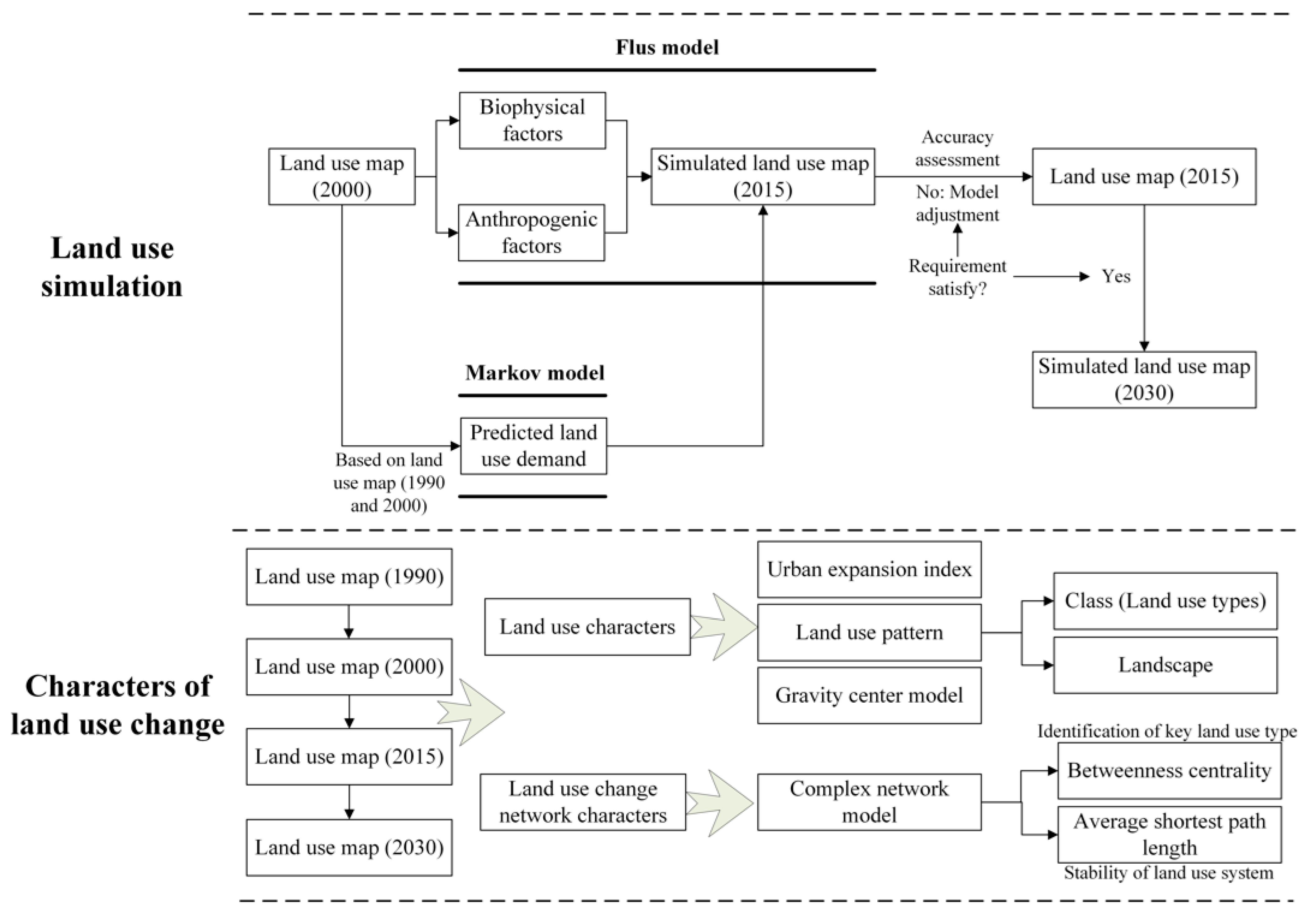
Figure 4.
Distribution of the land use in (a) 1990, (b) 2000, and (c) 2015.

Figure 5.
Simulation result of the land use cover change in 2030

Figure 6.
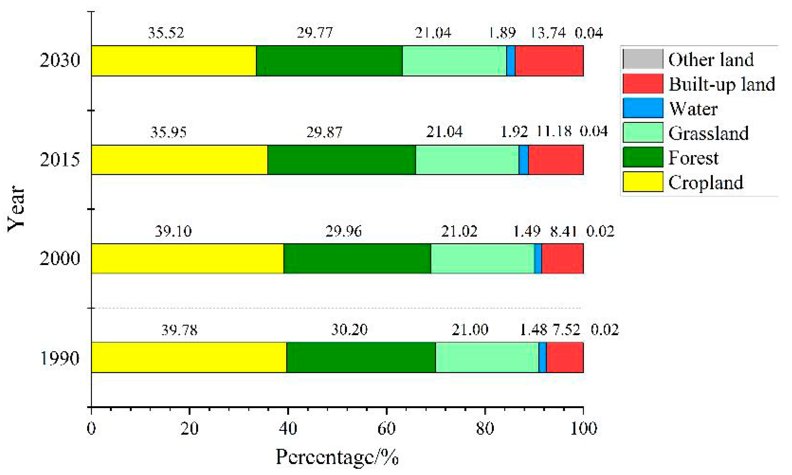
Percentage of the various land use types in 1990, 2000, 2015, and 2030.

Figure 7.
Movement of the built-up land gravity center during two periods.
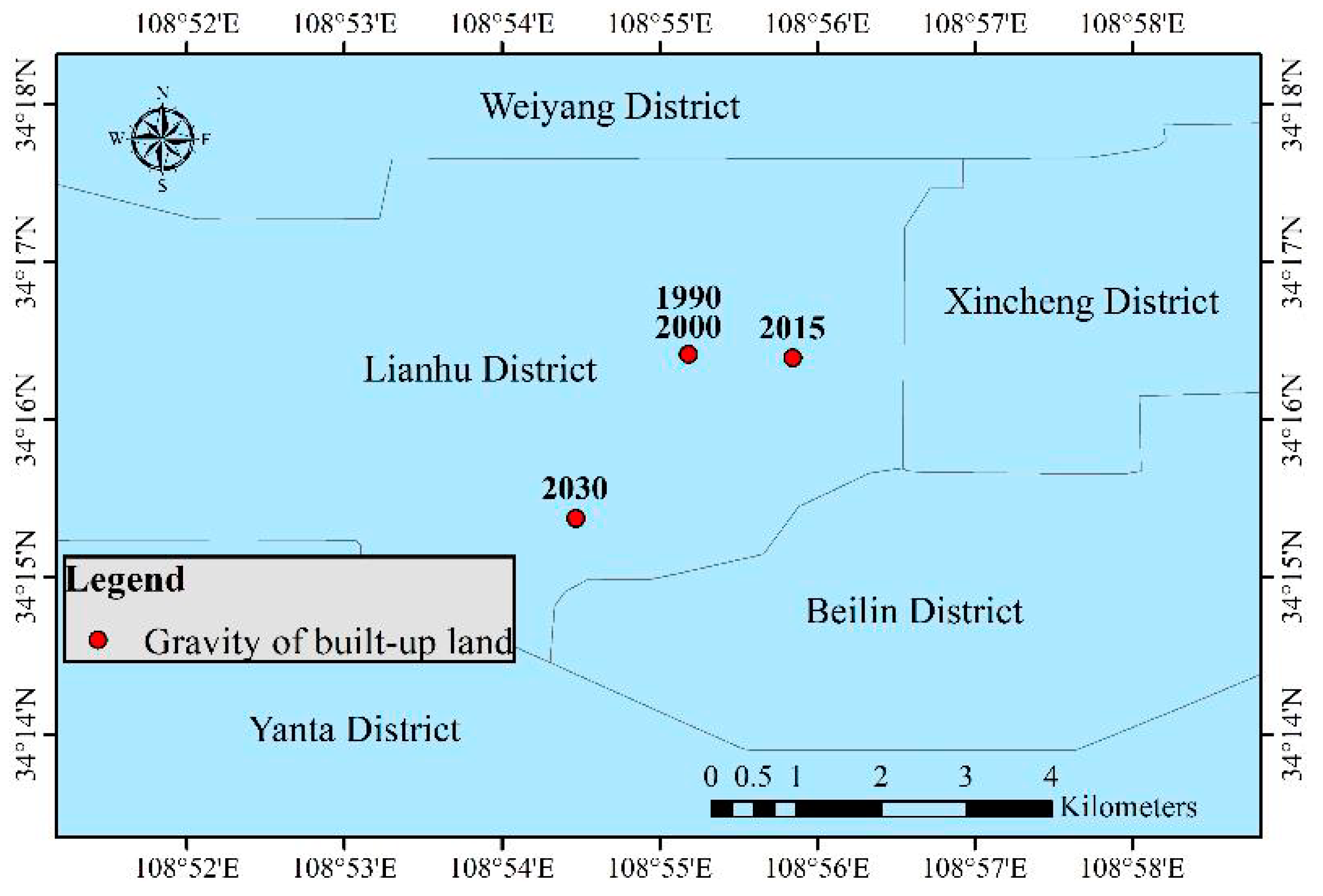
Figure 8.
Urban expansion index from 1990–2000, 2000–2015, and 2015–2030.

Figure 9.
Urban expansion index during the different periods.

Figure 10.
Changes in the land use pattern for the different land use types.

Figure 11.
Changes in the land use pattern characteristics at the landscape level in Xi’an.

Figure 12.
Complex network of the land use change in Xi’an city.

Figure 13.
Average shortest path during the different periods.

Table 1.
Source of the datasets.
| Datasets | Institution | Website |
|---|---|---|
| DEM | Geospatial Data Cloud site, Computer Network Information Center, Chinese Academy of Sciences | http://www.gscloud.cn |
| Slope | Calculated with the DEM | - |
| Soil texture | Resource and Environment Data Cloud Platform, Institute of Geographic and Natural Resources Research | http://www.resdc.cn/ |
| Temperature | ||
| Precipitation | ||
| Population density | Resource and Environment Data Cloud Platform, Institute of Geographic and Natural Resources Research | http://www.resdc.cn/ |
| Gross domestic product | ||
| Railway | National Catalogue Service for Geographic Information | http://www.webmap.cn/ |
| Road | Global Roads Open Access Data Set (gROADS), Socioeconomic Data and Applications Center | https://sedac.ciesin.columbia.edu/data/set/groads-global-roads-open-access-v1 |
| Rural settlement | National Catalogue Service for Geographic Information | http://www.webmap.cn/ |
| Urban center | Resource and Environment Data Cloud Platform, Institute of Geographic and Natural Resources Research | http://www.resdc.cn/ |
Table 2.
The selected factors of land use simulation.
| Category | Indicators | Resolution |
|---|---|---|
| Biophysical factors | Altitude | 90 m |
| Slope | 90 m | |
| Soil | ||
| Temperature | 1000 m | |
| Precipitation | 1000 m | |
| Anthropogenic factors | Population Density | 1000 m |
| Gross domestic product | 1000 m | |
| Distance to railway | Vector | |
| Distance to road | Vector | |
| Distance to rural settlement | Vector | |
| Distance to the urban center | Vector |
Table 3.
Selected land use pattern indicators.
| Types | Indicators |
|---|---|
| Class | Number of patches (NP), patch density (PD), largest patch index (LPI), landscape shape index (LSI), mean patch size (AREA_MN) |
| Landscape | Patch density (PD), number of patches (NP), largest patch index (LPI), Shannon’s diversity index (SHDI), mean patch area (AREA_MN), perimeter-area fractal dimension (FRAC_MN), mean patch shape index (SHAPE_MN), interspersion & juxtaposition index (IJI) |
Table 4.
Definitions of the indicators (landscape and class metrics) (Note: Referred from the User’s manual of Fragstats Version 4. http://www.umass.edu/landeco/research/fragstats/fragstats.html (2 February 2021)).
Table 4.
Definitions of the indicators (landscape and class metrics) (Note: Referred from the User’s manual of Fragstats Version 4. http://www.umass.edu/landeco/research/fragstats/fragstats.html (2 February 2021)).
| Types | Indicators | Definitions |
|---|---|---|
| Class | NP | Total number of a certain types. |
| PD | Number of patches in a given class, divided by the class area, multiplied by 10,000 and 100. | |
| LPI | Area of the largest patch of the corresponding patch type divided by the total landscape area, multiplied by 100. | |
| LSI | A quarter of the sum of the entire landscape boundary and all edge segments within the landscape boundary involving the corresponding patch type. | |
| AREA_MN | Mean value, across all patches of the corresponding patch types, of the corresponding patch metrics, divided by the number of patches of the same type. | |
| Landscape | PD | Number of patches in the landscape, divided by the total landscape area, multiplied by 10,000 and 100. |
| NP | Number of patches in the total landscape. | |
| LPI | Area of the largest patch of the corresponding patch type divided by the total landscape area. | |
| SHDI | Negative value of the sum, across all patch types, of the proportional abundance of each patch type multiplied by the proportion. | |
| AREA_MN | Mean value, across all patches of the corresponding patch types, of the corresponding patch metrics in the landscape. | |
| FRAC_MN | Two divided by the slope of the regression line obtained by regressing the logarithm of the patch area against the logarithm of the patch perimeter. | |
| SHAPE_MN | Mean value of the patch perimeter divided by the square root of the patch area, adjusted by a constant to adjust for a square standard. | |
| IJI | Negative value of the sum of the length of each unique edge type divided by the total landscape edge, multiplied by the logarithm of the same quantity, summed over each unique edge type. |
Table 5.
Accuracy of land use change simulation.
| Land Use Type | Producer Accuracy | User Accuracy | Kappa Coefficient |
|---|---|---|---|
| Cropland | 0.932584 | 0.932584 | 0.922535 |
| Forest | 0.980456 | 0.98366 | |
| Grassland | 0.981221 | 0.972093 | |
| Water | 0.764706 | 0.928571 | |
| Built-up land | 0.831776 | 0.816514 | |
| Other land | 1 | 1 |
Table 6.
Weighted indegree and weighted outdegree from 1990–2000.
| Land Use Type | Weighted Indegree | Weighted Outdegree | Weighted Indegree/Weighted Outdegree |
|---|---|---|---|
| Cropland | 3915 | 3983 | 0.983 |
| Forest | 3000 | 3024 | 0.992 |
| Grassland | 2105 | 2103 | 0.999 |
| Water | 149 | 148 | 1.001 |
| Built-up land | 842 | 753 | 1.118 |
| Other land | 2 | 2 | 1.000 |
Table 7.
Weighted indegree and weighted outdegree from 2000–2015.
| Land Use Type | Weighted Indegree | Weighted Outdegree | Weighted Indegree/Weighted Outdegree |
|---|---|---|---|
| Cropland | 3600 | 3915 | 0.920 |
| Forest | 2991 | 3000 | 0.997 |
| Grassland | 2107 | 2105 | 1.001 |
| Water | 192 | 149 | 1.289 |
| Built-up land | 1119 | 842 | 1.329 |
| Other land | 4 | 2 | 2.000 |
Table 8.
Weighted indegree and weighted outdegree from 2015–2030.
| Land Use Type | Weighted Indegree | Weighted Outdegree | Weighted Indegree/Weighted Outdegree |
|---|---|---|---|
| Cropland | 3356 | 3600 | 0.932 |
| Forest | 2981 | 2991 | 0.997 |
| Grassland | 2107 | 2107 | 1.000 |
| Water | 189 | 192 | 0.984 |
| Built-up land | 1376 | 1119 | 1.230 |
| Other land | 4 | 4 | 1.000 |
Table 9.
Betweenness Centrality of the land use change from 1990–2000.
| Land Use Type | Betweenness Centrality |
|---|---|
| Cropland | 8.0 |
| Forest | 0.0 |
| Grassland | 0.0 |
| Water | 0.0 |
| Built-up land | 0.0 |
| Other land | 0.0 |
Table 10.
Betweenness Centrality of the land use change from 2000–2015.
| Land Use Type | Betweenness Centrality |
|---|---|
| Cropland | 7.0 |
| Forest | 1.5 |
| Grassland | 1.83 |
| Water | 0.33 |
| Built-up land | 0.33 |
| Other land | 0.0 |
Table 11.
The Betweenness Centrality of land use change from 2015–2030.
| Land Use Type | Betweenness Centrality |
|---|---|
| Cropland | 0.0 |
| Forest | 0.0 |
| Grassland | 0.0 |
| Water | 0.0 |
| Built-up land | 0.0 |
| Other land | 0.0 |
Publisher’s Note: MDPI stays neutral with regard to jurisdictional claims in published maps and institutional affiliations. |
© 2021 by the authors. Licensee MDPI, Basel, Switzerland. This article is an open access article distributed under the terms and conditions of the Creative Commons Attribution (CC BY) license (http://creativecommons.org/licenses/by/4.0/).
Share and Cite
MDPI and ACS Style
Feng, D.; Bao, W.; Fu, M.; Zhang, M.; Sun, Y. Current and Future Land Use Characters of a National Central City in Eco-Fragile Region—A Case Study in Xi’an City Based on FLUS Model. Land 2021, 10, 286. https://doi.org/10.3390/land10030286
AMA Style
Feng D, Bao W, Fu M, Zhang M, Sun Y. Current and Future Land Use Characters of a National Central City in Eco-Fragile Region—A Case Study in Xi’an City Based on FLUS Model. Land. 2021; 10(3):286. https://doi.org/10.3390/land10030286
Chicago/Turabian StyleFeng, Dingrao, Wenkai Bao, Meichen Fu, Min Zhang, and Yiyu Sun. 2021. "Current and Future Land Use Characters of a National Central City in Eco-Fragile Region—A Case Study in Xi’an City Based on FLUS Model" Land 10, no. 3: 286. https://doi.org/10.3390/land10030286
Note that from the first issue of 2016, this journal uses article numbers instead of page numbers. See further details here.