A Preliminary Study on the Impact of Landscape Pattern Changes Due to Urbanization: Case Study of Jakarta, Indonesia

Abstract

Urbanization is changing land use–land cover (LULC) transforming green spaces (GS) and bodies of water into built-up areas. LULC change is affecting ecosystem services (ES) in urban areas, such as by decreasing of the water retention capacity, the urban temperature regulation capacity and the carbon sequestration. The relation between LULC change and ES is still poorly examined and quantified using actual field data. In most ES studies, GS is perceived as lumped areas instead of distributed areas, implicitly ignoring landscape patterns (LP), such as connectivity and aggregation. This preliminary study is one of the first to provide quantitative evidence of the influence of landscape pattern changes on a selection of urban ecosystem services in a megacity as Jakarta, Indonesia. The impact of urbanization on the spatiotemporal changes of ES has been identified by considering connectivity and aggregation of GS. It reveals that LP changes have significantly decreased carbon sequestration, temperature regulation, and runoff regulation by 10.4, 12.4, and 11.5%, respectively. This indicates that the impact of GS on ES is not only determined by its area, but also by its LP. Further detailed studies will be needed to validate these results.

1. Introduction

The urban population had increased to 3.9 billion (54% of the total population) by 2014 and will increase to around 6.3 billion (67% of the total population) by 2050 [1]. Population increase drives land use–land cover (LULC) change transforming green spaces as well as bodies of water into built-up areas resulting in decrease and loss of ecosystem services (ES) in urban areas [2,3,4,5]. Ecosystem services are the varied benefits to humans from the natural environment and healthy ecosystems. They can be categorized as provisioning services, regulating services, cultural services, and supporting services [6]. A city or an urban area can be seen as a single ecosystem where the urban population directly benefits from ecosystem services generated by urban ecosystems, such as green and blue infrastructure [7]. Ecosystem services in urban areas include air quality improvement, noise reduction, controlling air temperature, carbon storage and sequestration, water regulation, and recreation [7,8,9,10,11,12,13] and therefore enhance citizens well-being [14,15].

Many studies show that urbanization and LULC change are key anthropogenic drivers affecting urban ecosystem’s functions and services [11,16,17,18,19]. Some examples of the impact of LULC change on ES due to urbanization are a decrease in the capacity to retain stormwater leading to urban flooding [20], and an increase in the land surface temperature (LST) [21] in cities. Yuan et al. [22] showed that in Nanjing, China, there was a decrease in the provision and delivery of supply services, the supporting services, and the regulating services by 17, 0.9, and 4.3%, respectively, due to urbanization between 2000 and 2015. In Beijing, urban growth between 1985 and 2015 decreased carbon storage and water yield by 3.3 and 4%, respectively, while sediment export increased by 15.5% (Sun et al., 2018b). Another study from Atlanta Metropolitan area, US, showed that urban expansion between 1985 and 2012 reduced carbon storage by 23% and water purification capacity by 28 and 49%, for nitrogen and phosphorus, respectively, but increased sediment transport by 17% (Sun et al., 2018). Jaligot et al. [23] showed that the cultural services in Yaoundé, Cameroon, decreased by more than 90% due to urbanization between 2000 and 2018. LULC change from 1990 to 2017 in the West Bengal, India, resulted in some of the regulating services increasing while others decreased. Water regulation, water supply, and waste treatment increased by 57, 22, and 8%, respectively, while climate regulation and nutrient cycling decreased by 31.82 and 31.25%, respectively [24].

The relationship between urbanization, LULC change, and ES has been studied from various perspectives. Panagopoulos et al. [14] discussed the importance of urban ES and landscape planning to sustainable urban development. Das and Das [24] investigated the impact of LULC change on ES by quantifying the total ecosystem service value (ESV) based on the area of the ecosystem, and a value coefficient (VC) [25]. The extension of built-up areas in West Bengal decreased agricultural and vegetation covers. As a result, the total ESV of landscape decreased by 24.30% from 1990 to 2017. Wang et al. [26] investigated the impact of urbanization from 2000 to 2010 on multiple ES at hotspots and urban megaregion scale of Beijing–Tianjin–Hebei (BTH), the capital economic zone of China, by considering three components of urbanization: the built-up area proportion, the population density, and the gross domestic product (GDP) density. The ES in their study was calculated using the area of the ecosystem, for instance, the total food production was based on the area of cropland. It was revealed that providing services of food supply had an “inverse U” shape relation with the population and the GDP density, while urban expansion decreased regulating services. The impact of urbanization on ES was not only influenced by an increase in urban areas or a decrease in green spaces but also by landscape pattern changes, such as a number of patches (NP), aggregation index (AI), and “clumpiness” index, as discussed by Asadolahi et al. [27]. The ecosystem services in their study were based on the area of ecosystems, including water body, agriculture, rangeland, forest, and urban. Moreover, the influence of landscape patterns to ES provision was analyzed by comparing the landscape metric changes and ES. They saw that increasing food supply had a positive correlation with the good connectivity and connectedness of agricultural land. Haas et al. [28] discussed the relationship between a decrease in ES with an increase in built-up areas and landscape pattern changes due to urbanization in the period from 1989 to 2001 in Stockholm and Shanghai. They observed that an increase in built-up areas along with landscape pattern changes, such as a decrease in connectivity, an increase in fragmentation, and more complex shapes of the natural landscape, had a negative impact on ES. The ES in their study was based on the area of ecosystems, such as wetland, water, forest, agriculture, urban green space, high-density building, and low-density building. Moreover, the relationship between ES and landscape pattern changes was discussed by comparing the changes of the landscape metrics and ES. For urban flood mitigation, Bai et al. [29] conducted a field survey study in Luohe, China, which observed that inundated areas had a low proportion of green spaces and bare land. Moreover, landscape metrics analysis showed that the mean patch size of green spaces of flooded areas was smaller compared with that of roofs. Meanwhile, the connectivity of green spaces had no significant contribution to mitigating urban flooding. The importance of landscape patterns on surface runoff control was also observed by [30]. They directly integrated large patch index (LPI) and aggregation index (AI) of green spaces with runoff coefficients to estimate runoff volume controlled in Beijing, China. It was found that increasing runoff was related to a decrease in green spaces, as well as increasing the fragmentation and disaggregation of green spaces. The landscape patterns can also exhibit a relation with an increase in LST in the Olympic forest park of Beijing, China, as investigated by using the Pearson correlation analysis [31]. It was revealed that an increase in LST was related to increasing urbanization in the period 2000 to 2015. Moreover, there was a negative correlation between LST and the landscape metrics of large patch index (LPI) and aggregation index (AI) of green spaces.

A growing number of studies have investigated the impact of urbanization and LULC change on ES. These studies reveal that a decrease in green spaces affects ES, feeding the perception that there is a positive relationship between the surface area of green spaces and urban ecosystem functioning [4,32]. However, these studies generally ignore the impact of spatial heterogeneity of the land surfaces as they lump together the area of each land-use type. Only a few of them acknowledged the differences in landscape patterns but still did not consider landscape patterns in calculating the impact of green spaces. As a result, an area of green spaces, as shown in Figure 1, could still be perceived as a lumped area instead of a distributed area, where the green space units have different landscape patterns, such as connectivity, aggregation, mean patch size, and large patch index, which could affect ecosystem services [33,34].

In many existing studies, the impact of urbanization and LULC change on ES is generally discussed using the lumped area of green spaces. Some studies have discussed the impact by comparing the ES changes and the changes of landscape patterns, which show that landscape patterns can affect ES. However, there is a lack of studies that directly examine the impact of landscape pattern changes on the area of green spaces to ES calculation.

This preliminary study aims to identify the impact of landscape pattern changes on urban ecosystem services using two spatial configurations of green spaces, as shown in Figure 1. Firstly, the area of green spaces is assumed as a lumped area, as depicted in Figure 1b. Secondly, the area of green spaces is assumed as a distributed area, as shown in Figure 1a, which is represented by directly combining the area and landscape patterns defined by the aggregation and the connectivity of the green spaces and bodies of water. As a preliminary study, this study is designed to focus on the investigation of the landscape pattern changes and their influence on urban ES. It is expected that the results of this study can provide insight into the influence of landscape patterns on ES calculation. Moreover, the validation of the results is not a part of this study since there is a lack of field survey data for all municipalities in Jakarta. Hence, the validation would be considered as a part of further studies.

This study is divided into three main parts: (1) assessing the impact of urbanization on LULC change; (2) analyzing the impact of LULC change on the landscape patterns; and (3) analyzing the impact of the landscape pattern changes on ecosystem services.

2. Materials and Methods

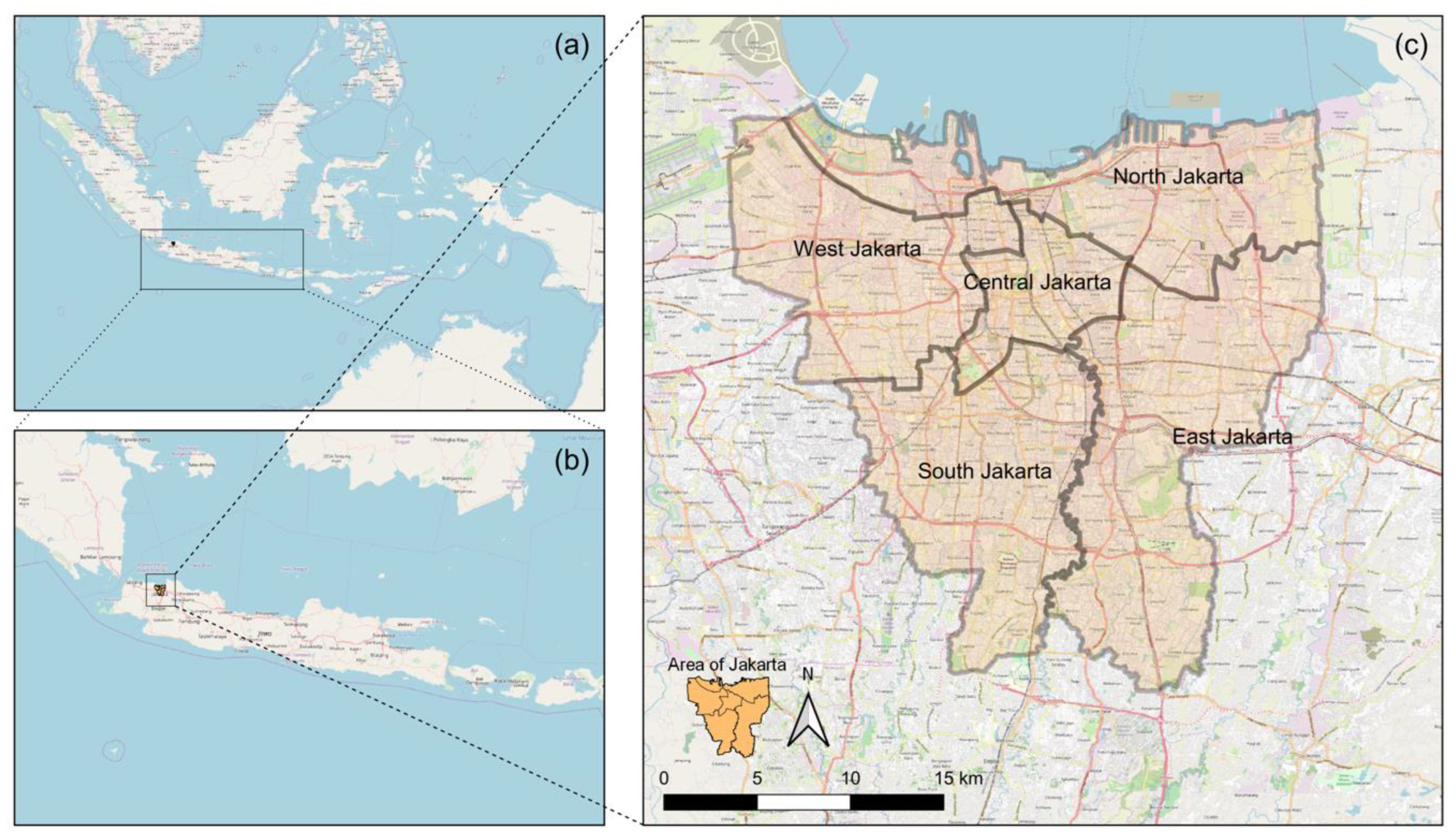
This study was carried out in Jakarta, Indonesia, and it was conducted in six steps. First, LULC maps for 1995 and 2014 were generated using Landsat images. The LULC classification used six LULC classes, which were urban, suburban, grassland, cropland, trees, and water (sea and surface water). Second, the results of LULC classification were imported into the FRAGSTATS, the spatial pattern analysis program, for landscape metric analysis. The analysis considered four landscape metrics and the relationship between them: Class Area (CA), Land Proportion (PLAND), Aggregation Index (AI), and connectivity (COHESION). The landscape metrics analysis was carried out for five municipalities of Jakarta. Third, the impact of urbanization on LULC change was analyzed, which was based on the CA of LULC classes. Fourth, the impact of LULC change on the landscape patterns was analyzed, which was based on PLAND, AI, and COHESION. Fifth, ecosystem services were calculated using two methods: area-based estimation and landscape metric area (LMA). The area-based estimation followed commonly ecosystem services area calculation that uses only the area of green spaces, while the landscape metric area directly incorporated the landscape metric representing the spatial characteristic/configuration of green spaces to ecosystem services area calculation. Sixth, ecosystem services changes between 1995 and 2014 from two different methods were then analyzed using ecosystem services index (ESI).

2.1. Study Area

Jakarta is the capital of Indonesia, which has experienced rapid urbanization and the extensive transformation of vegetative green spaces into impermeable urban surfaces [35,36,37,38]. Urbanization in Jakarta is driven by several factors, including its strategic political and economic position as the capital city where important activities like the functions of the national government, education, manufacturing, and commerce are taking place [39]. Jakarta has six municipalities, which are Central Jakarta, North Jakarta, West Jakarta, South Jakarta, and East Jakarta, as shown in Figure 2, and one regency, which is the Thousand Islands (not shown in the figure). This study focuses on the municipalities that consist of 42 subdistricts, which are home of approximately 10 million people, with the population growth rate of 1.02% per year in 2015 [40]. East Jakarta is the most populated area, whereas West Jakarta is the most densely populated area with a population density of 19,018 per km². Located on the northwest coast of Java, Jakarta’s climate is a tropical monsoon climate according to the Köppen climate classification system and it has two seasons, which are the rainy season from October through May and the dry season from June to September. During the rainy season, the average monthly rainfall is 300 mm, while it is 43 mm in August during the dry season [40].

2.2. Data Sources

The impact of urbanization on LULC change was analyzed using land use–land cover maps of Jakarta for the year 1995 and 2014. The maps were prepared using Landsat images selected for the area of Jakarta and its surrounding. For the year 1995, the Landsat 5 TM L1TP from 24 August 1995, was used, while the Landsat 8 OLI TIRS L1TP obtained on 13 September 2014, was selected for the land use–land cover map of the year 2014. Both datasets had 30 m resolution. The land cover classification was based on the land cover classes used to investigate the relationship between green spaces and increasing urban temperature [41]. We used the semiautomatic classification in QGIS [42], a free and open-source geographic information system, to generate six land cover classes: urban, suburban, grassland, cropland, trees, and water. An urban area is an area where there is a dense mix of compact high-rise, compact midrise, or low-rise buildings, while a suburban area is an open arrangement of low-rise buildings with pervious land covers, such as grass, low plants, and scattered trees. A grassland area is defined as an area where the vegetation is dominated by grasses, and there are few or no other plants. A cropland area is an area mainly used for agricultural and farming purposes, where rice, corn, vegetables, and fruits are grown. An area of trees is an area where trees are dominant. Water represents both sea and surface water, such as rivers and lakes. Moreover, the LULC change analysis was based on the CA from five land cover classes: urban, trees, grassland, cropland, and bodies of water.

The boundary area of Jakarta and its municipalities was obtained online from the Geospatial Information Agency of Indonesia (BIG) database, www.tanahair.indonesia.go.id (accessed on 20 September 2019).

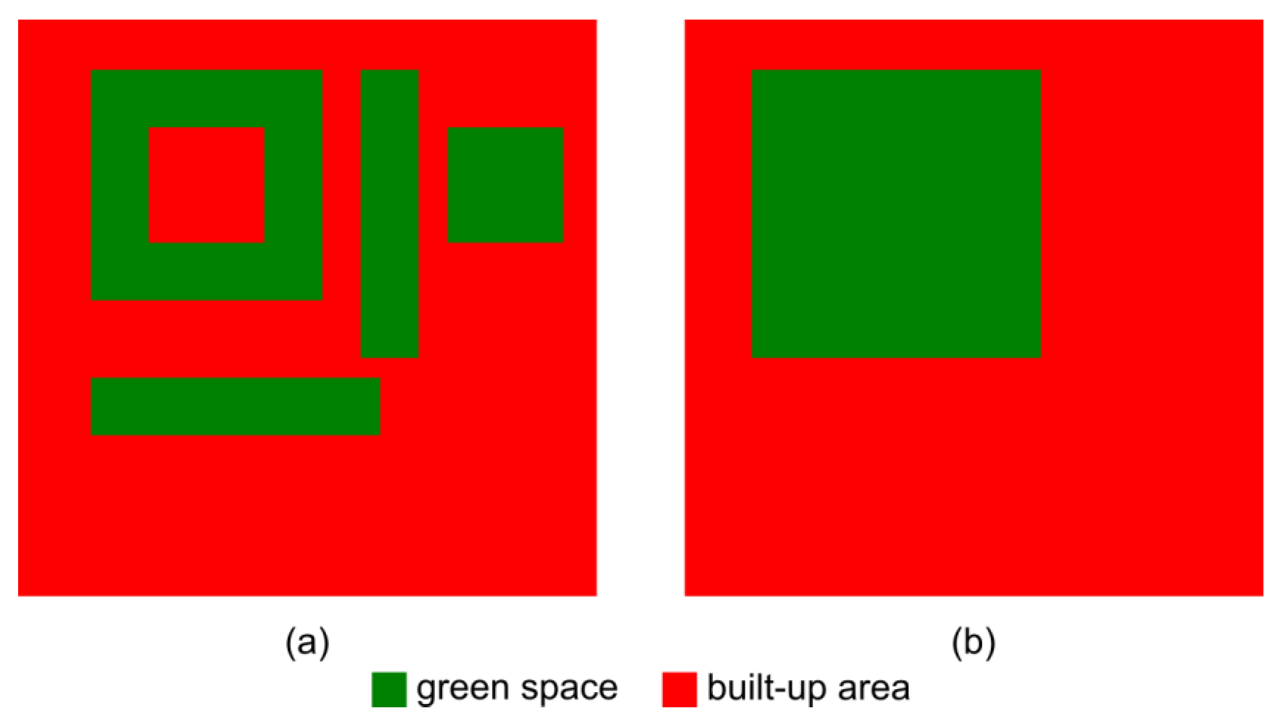
2.3. Landscape Metrics

Landscape metrics are quantified characteristics of the spatial pattern at different levels (i.e., patch level, class level, and landscape-level) used to describe landscape structures and LULC change [43,44,45]. Information about landscape structures is essential to analyze ecosystem structures, functions, and services [46] and to evaluate their spatial effects at the patch–class–landscape level [47,48]. Patch level metrics are important for defining individual patches and for characterizing the spatial context of the patches, which are used as the computational basis for other landscape metrics. At the class level, the metrics are calculated by integrating all patches from a given class. The class level calculation can be done by a simple aggregation of the area of patches to reflect the total area of a given class. Moreover, landscape-level metrics are the integration of all classes over the landscape [49]. This study uses four landscape metrics to capture the spatial features which affect urban ecosystem processes: class area (CA), connectivity (COHESION), land proportion (PLAND), and aggregation index (AI). CA is a measure of landscape composition; specifically, to indicate how much of the landscape is comprised of a patch type. The class area is the primary component used in the ecosystem service quantification [45]. The connectivity of a class is measured by the patch cohesion index (COHESION) that measures the physical connectedness of the corresponding patch type. Patch cohesion increases as the patch type become more clumped or aggregated in its distribution; hence, more physically connected [50]. The decrease in patch connectivity in a landscape could be a negative sign for ecosystem services [28]. The land proportion (PLAND) is the percentage of a landscape, which quantifies the proportional abundance of each patch type in the landscape, while the AI is used to understand the spatial aggregation of a patch in a landscape [31,45,51]. The landscape metrics in this study were calculated using FRAGSTATS 4.2, the spatial pattern analysis program, which is developed by McGarigal and Cushman of University of Massachusetts in the United States of America [48].

The landscape metrics used in this study were selected based on the premise that there is a correlation between ES and the area, the aggregation, and the connectivity of ecosystem [31,45,52]. In general, many ES studies focus on the relationship between ecosystem services and the area of green spaces revealing a positive correlation between the size of the green spaces and the weight of the ecosystem services provided [53,54,55]. However, some studies showed that ecosystem services were also influenced by landscape patterns [29,30,55,56]. In this study, ES was analyzed by considering the “effective area” of green spaces and bodies of water by taking into account the influence of aggregation and connectivity on the area of green spaces and bodies of water. The landscape metric combinations for this study are selected based on the FRAGSTATS 4.2 guidelines and the existing research on landscape metric and ES. There are some indices that can be used to analyze the relationship between landscape metrics and ES, such as Number of Patch (NP), Patch Density (PD), Large Patch Index (LPI), patch cohesion index (COHESION), land proportion (PLAND), CONTAGION, and Aggregation Index (AI). Among them, the AI was selected because it can give more accurate results compared to that of other aggregation indices, such as CONTAGION [51], while the COHESION was selected for connectivity analysis because it can represent the connectivity of a corresponding patch type of a particular class [28,50]. This resulted in the “Landscape Metric Area” (LMA) calculated by multiplying the metrics class area (CA), aggregation index (AI), and cohesion index (COHESION) for each land cover class, as follows:

$$LMA=CA\times AI\times COHESION$$

(1)

LMA was calculated at the municipality level following the Indonesian regulation for spatial planning. The standard focuses on the city level and defines the spatial configuration of different land use–land cover types, including the minimum proportion of open green spaces [57].

2.4. Urban Ecosystem Services

Many studies discussed ES in urban areas [7,9,28,45,58,59]. Back in the 1990s, one of the pioneering urban ecosystem services studies considered six ecosystem services: air filtering, microclimate regulation, noise reduction, rainwater drainage, sewage treatment, and recreation [7]. Derkzen et al. [9] studied ecosystem services bundles in Rotterdam, the Netherlands, considering six ecosystem services: air purification, carbon storage, noise reduction, runoff regulation, cooling, and recreation. The importance of urban ecosystem services inspires local and national governments to incorporate ES in their urban planning process and documents [58,60,61,62]. For example, the government of Indonesia requires a minimum of 30% open green spaces in each city and urban area [57,63].

In this study, ES changes analysis was limited to carbon sequestration, temperature regulation, and runoff regulation, due to the limitation of the medium resolution satellite images to capture several urban details, such as street corridors and small city parks. Furthermore, in the ES selection increasing carbon emissions [64,65], and recent climate-related hazard events in Jakarta, such as urban flooding in 2013, 2014, 2015, and 2020, have also been considered [66,67], as well as the potential increase in the urban temperature [37,68]. The ES estimation adopted a weighting factor used in [9], where the green space with high-temperature regulation capacity was given a weight of 1.0, whereas 0.5 was given for low capacity. In this study, the weighting factor was implemented for all ES estimations for which the factor was given on the basis of the importance of a particular green space to a particular ES. For example, grassland was given the weight of 0.5 for temperature regulation, but it was given 1.0 of the weight factors for runoff regulation.

2.4.1. Carbon Sequestration

Green spaces have an important role in the carbon cycle, capturing CO₂ from the atmosphere during photosynthesis, and releasing it during respiration. In an urban area, carbon sequestration mainly takes place in green spaces [69,70,71]. Each green space has a different carbon sequestration rate, and urban trees generally have a higher rate compared to that of other green spaces because of their higher leaf area index (LAI), which is the ratio of the area of trees’ leaves per area of the land surface [72]. For example, the urban forest of Punggol forest in Singapore had the annual carbon sequestration rate of 1.6 ton/year/ha, where trees with high LAI such as Delonix regia and Artocarpus heterophyllus gave a significant contribution [53]. Studies from Indonesian cities showed that trees had a carbon sequestration rate higher than that of other vegetation, including grass and herbaceous. For instance, the carbon sequestration of tree-covered areas in a part of Jakarta was 129.92 kg/ha/hour, much higher than 2.74 kg/ha/hour for grass areas [73]. Moreover, trees in the city of Singaraja on Bali island had 112.751 tons/ha of carbon sequestration higher than 4.845 tons/ha of carbon sequestration of herbaceous [74].

In this study, carbon sequestration was based on the LMA of trees. The LMA of trees was given a weight of 1.0 considering its carbon sequestration, which is higher than that of other vegetation. Other types of green spaces were given a weight of 0, assuming no significant contribution to capturing carbon in the atmosphere.

2.4.2. Temperature Regulation

Increasing LST and air temperature in urban areas can be influenced by several factors, including a decrease in green spaces and bodies of water. The contribution of green spaces to the control of urban temperatures can be achieved through ecosystem functions such as evapotranspiration, trees shading, and modifying air movement, while the greatest contributing factor to the cooling effect is shading and evapotranspiration [75]. The effectivity of green spaces in providing the ecosystem functions is influenced by various factors, including the area and the spatial distribution of green spaces [76], the configuration and the shape of green spaces [52,77], and the connectivity of green spaces [31]. Among green spaces, trees have high cooling potential through shading and evapotranspiration, while other short vegetative covers such as grass and crops might have a lower capacity [9,78]. The temperature in urban areas can also be regulated through evaporation and heat absorption from bodies of water [79]. The cooling effect of bodies of water is influenced by the area of the bodies of water [80], and the effect decreases with the increase in distance from the water body, which is similar to the cooling effect from green spaces [81,82].

Temperature regulation in this study was estimated using the combination of the LMA from trees, grassland, cropland, and bodies of water. The LMA of trees was given a weight of 1.0, while a weight of 0.5 was given for the LMA of grassland, cropland, and bodies of water.

2.4.3. Runoff Regulation

Due to urbanization, cities and urban areas are more vulnerable to urban flooding. The increasing vulnerability is influenced by some factors such as a decrease in green spaces and bodies of water. As a result, many urban areas have an insufficient capacity for infiltration and interception, as well as an increase in the runoff coefficient. Urban flooding-related studies showed that the area of green spaces could be considered as one of the important factors that determine runoff regulation [30,83,84]. For instance, increasing tree-cover by nearly 11% in Beijing could increase the total runoff reduction volume by more than 30% [85]. Moreover, the capacity of green spaces in controlling surface runoff is also influenced by several factors, including the interception of rainfall. Among many types of green spaces, trees could provide the high interception capacity, particularly in the short–moderate rainfall or in the earlier periods of precipitation, and it decreases in the longer duration or during high rainfall intensity [86]. A field experiment from the city of Uruaçu, Goiás, Brazil, showed that interception rate during short, low-intensity precipitation was about 40%, while the rate was about 3.6% in the high intensity and long duration rainfall [87]. Besides interception, green spaces also provide runoff regulation through infiltration, which is influenced by numerous factors including rainfall intensity, green space types, soil characteristics, and green space coverage [19,88,89,90]. In addition, green spaces contribute to runoff coefficients by increasing flow resistance, which can be associated with its density [91]. Furthermore, bodies of water like rivers, lakes, and wetlands also have the potential to control surface runoff through storage functions [83].

The estimation of runoff regulation service in this study considered the combination of the LMA from trees, cropland, grass, and bodies of water. All green spaces were given a weight of 1.0 based on the assumption that green spaces and bodies of water had a similar contribution to runoff regulation from one or the combination of infiltration, interception, flow resistance, and storage functions.

2.5. Ecosystem Services Index (ESI)

This study used ecosystem services index (ESI) to assess the ES changes. The ESI was based on the ES calculated using the combination of the LMA from green spaces and bodies of water. The ES calculation was divided into two steps. First, the ES was only based on the area of green spaces and bodies of water called area-based estimation. Second, the ES was based on the LMA calculated using the following equation.

$$ES=aLM{A}_{tree}+bLM{A}_{grassland}+cLM{A}_{cropland}+dLM{A}_{water}$$

(2)

where a, b, c, and d were the weighting factors for each green space and bodies of water. The weighting factor was different for each green space in each ES estimation, as given in

Table 1. The weighting factors (modified from Derkzen et al. [9]).

Weighting Factors	Carbon Sequestration	Temperature Regulation	Runoff Regulation
a (Trees)	1	1	1
b (Grassland)	0	0.5	1
c (Cropland)	0	0.5	1
d (Water)	0	1	1

.

The ESI was then calculated by normalizing the ES values using the following formula:

$$ES{I}_{ij}=\frac{E{S}_{ij}-E{S}_{min}}{E{S}_{max}-E{S}_{min}}$$

(3)

where $ES{I}_{ij}$ is the index of ES, $i$ for the municipality $j$, $E{S}_{ij}$ is the value of ES, $i$ for the municipality $j$, and $E{S}_{min}$ and $E{S}_{max}$ are the minimum and the maximum value of ES $i$, respectively.

3. Results

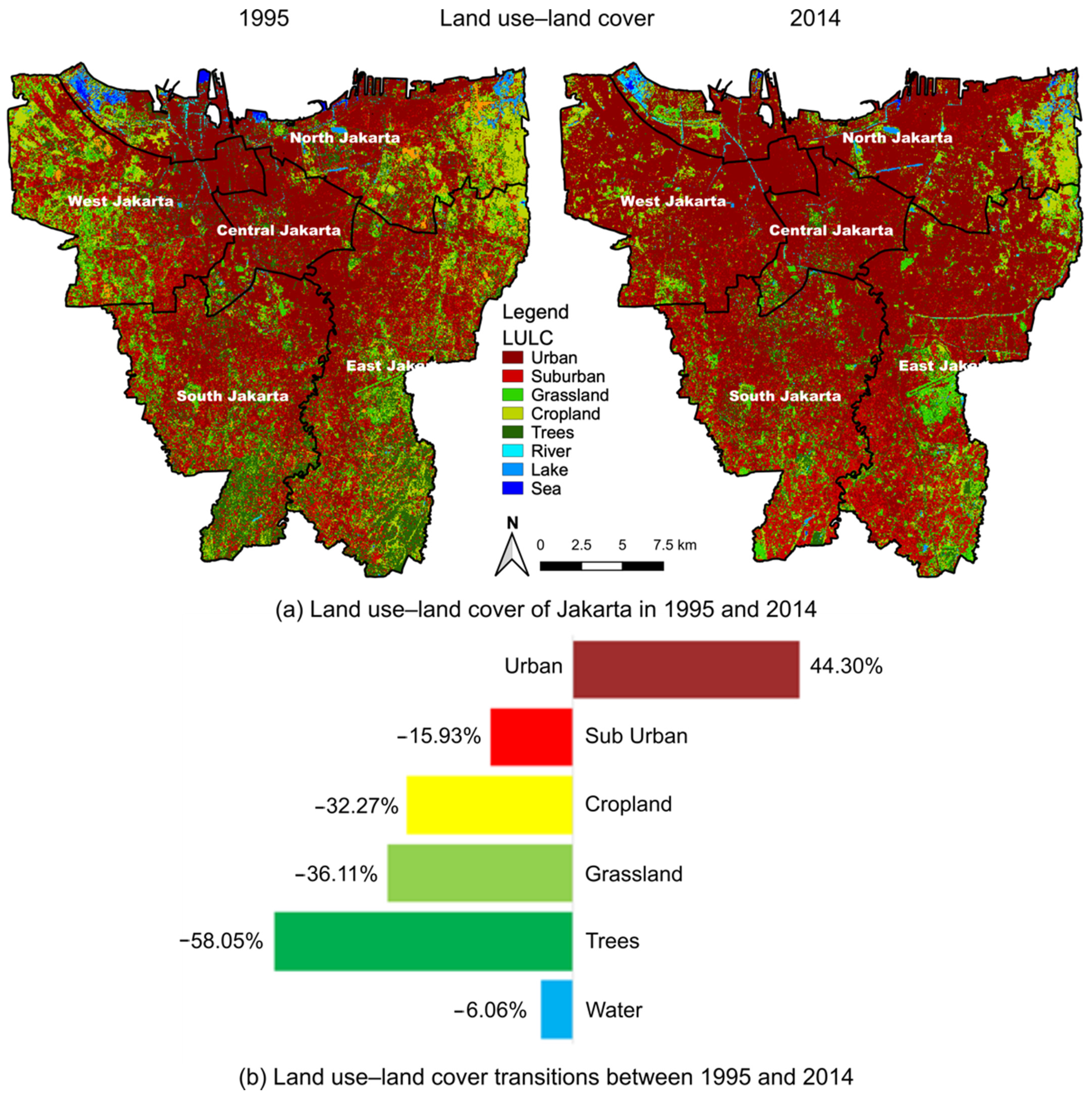
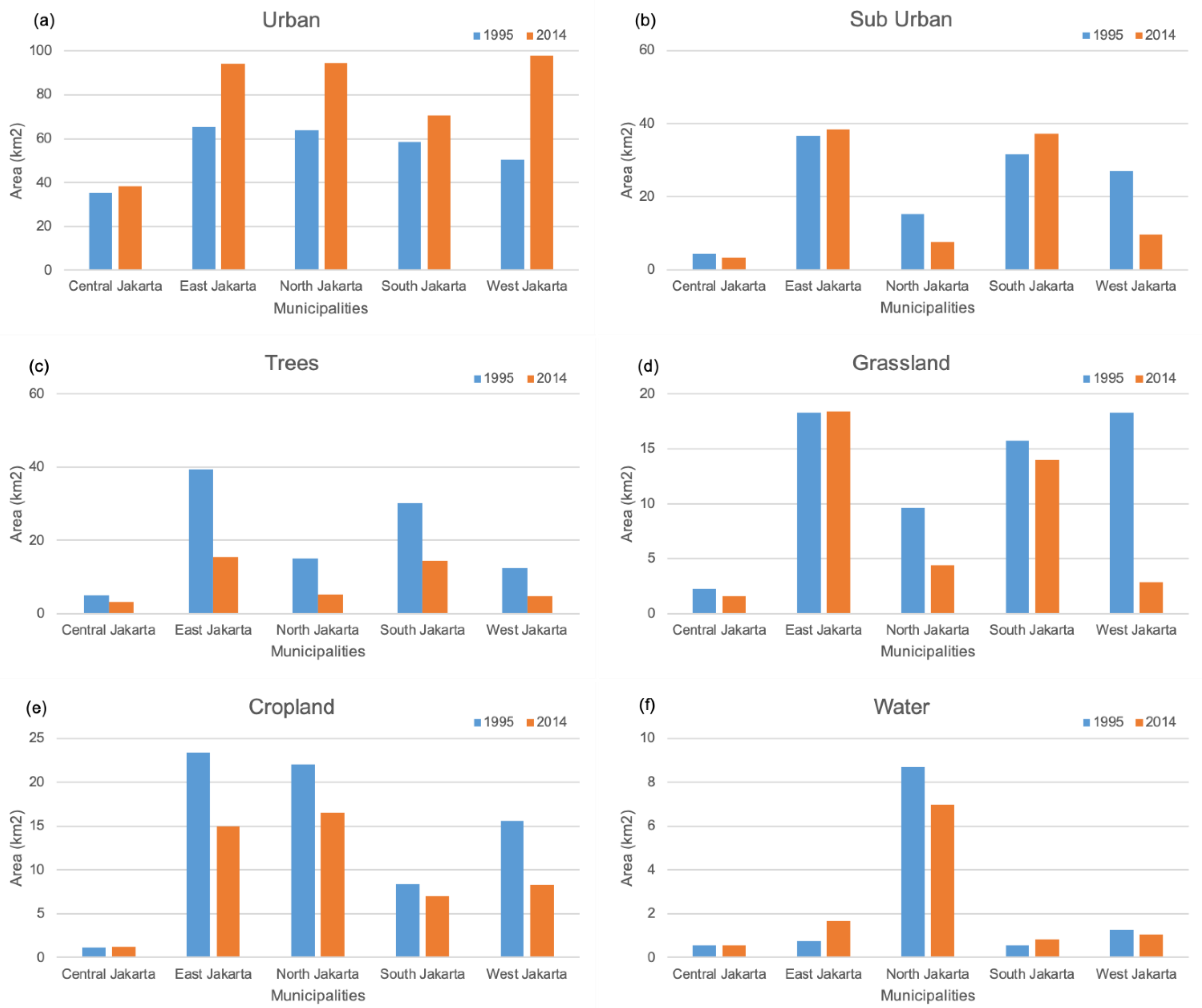
3.1. Land Use–Land Cover (LULC) Change Analysis

The high rate of land transformation marked urbanization in Jakarta from 1995 to 2014, as shown in Figure 3. It shows that there has been a substantial change in the spatial distribution of green spaces due to increasing urban areas. The growing urban areas, about 44.3%, lost about 58.1% of the areas with trees, 36.1% of grassland, 32.3% of cropland, 15.9% of suburban areas, and 6.1% of bodies of water (lakes and rivers).

The LULC change in the study was analyzed by focusing on the spatial extension of the urban areas and the decrease in vegetative cover and bodies of water from 1995 to 2014, as shown in Figure 4. In 1995, the spatial distribution of urban areas was concentrated in three municipalities, which were East Jakarta (65.3 km²), followed by North Jakarta (63.9 km²) and South Jakarta (58.5 km²). On the other hand, the smallest urban area was about 35.4 km², which was observed in Central Jakarta. After 20 years, urban areas increased in all municipalities. The largest urban area in 2014 was about 97.8 km² in West Jakarta, which increased by about 93.7% from that in 1995. Meanwhile, urban areas in East Jakarta and North Jakarta increased by almost a half from that in 1995. On the other hand, the smallest urban area, by approximately 38.4 km², was identified in Central Jakarta, which increased by 8.2%.

The increase in built-up areas was also observed in suburban areas from 1995 to 2014, as shown in Figure 4. In 1995, the largest suburban area was detected in East Jakarta (36.4 km²), followed by South Jakarta (31.6 km²) and West Jakarta (26.9 km²). Central Jakarta had the smallest suburban area by about 4.30 km². The spatial distribution of suburban areas in 2014 was a bit different from urban areas, which increased in all municipalities. The changes of suburban areas were marked by a decrease in West Jakarta (−64.0%), followed by North Jakarta (−51.0%) and Central Jakarta (−19.6%), but they increased in East Jakarta and South Jakarta. The largest suburban area of 38.37 km² was identified in East Jakarta, which increased by 5.3% from that in 1995. This increase, however, was lower than 17.7% in South Jakarta. On the other hand, the smallest suburban area of 3.4 km² was detected in Central Jakarta.

The dynamic changes of the built-up areas affected the area of green spaces, where trees were by far the most affected, followed by grassland and cropland, as shown in Figure 4 and Figure 5. In 1995, trees were mainly distributed in East Jakarta and South Jakarta, where the area of trees was more than two times of that in the other municipalities, such as in North Jakarta and West Jakarta. The largest area of trees (39.4 km²) was observed in East Jakarta, while the smallest area of 5.0 km² was in Central Jakarta. In 2014, the area of trees decreased above the average in all municipalities except in South Jakarta and Central Jakarta. A significant decrease of 65.8% was observed in North Jakarta, followed by West Jakarta (−62.2%) and East Jakarta (−61.1%). However, the area of trees in that area was still higher than that in other municipalities. For instance, East Jakarta had the largest area of trees (15.4 km²), which was higher than 14.5 km² in South Jakarta. On the other hand, the smallest area of trees (3.2 km²) was detected in Central Jakarta.

Besides trees, areas of grassland were also impacted by an increase in the built-up areas, as depicted in Figure 4 and Figure 5. In 1995, the widespread occurrence of areas of grassland was mainly detected in East Jakarta, West Jakarta, and South Jakarta. The largest grassland area (18.3 km²) was observed in East Jakarta, which was similar to that of West Jakarta. On the other hand, Central Jakarta had the smallest area of about 2.3 km². In 2014, the grassland area remained almost the same in East Jakarta, while a significant decrease of 84.5% was observed in West Jakarta, followed by North Jakarta (−54.5%). The smallest area of grassland was observed in Central Jakarta (1.6 km²), followed by West Jakarta (2.8 km²) and North Jakarta (4.4 km²).

A decrease in the area of green spaces was also found in the area of cropland during urbanization from the year 1995 to 2014, as shown in Figure 4 and Figure 5. The spatial distribution of cropland in 1995 was dominant in East Jakarta and North Jakarta, where the areas of cropland were 23.4 km² and 22.1 km², respectively. In 2014, there was a decrease in the area of cropland. The highest decrease was identified in West Jakarta, where the area of cropland decreased by 47.1%, followed by East Jakarta (−35.9%) and North Jakarta (−25.2%). Moreover, the spatial distribution of cropland in 2014 was similar to that in 1995, where the dominant distribution of cropland was observed in North Jakarta (16.5 km²), followed by East Jakarta (14.9 km²).

The existence of bodies of water between 1995 and 2014 was identified by a small decrease by −6.1%, as shown in Figure 4 and Figure 5. The spatial distribution of the bodies of water was mainly observed in North Jakarta, representing lakes, fishponds, and wetlands. As a result, North Jakarta had the largest area of bodies of water between 1995 and 2014, where small patches of bodies of water, including rivers, creeks and small wetlands, were evenly distributed in all municipalities.

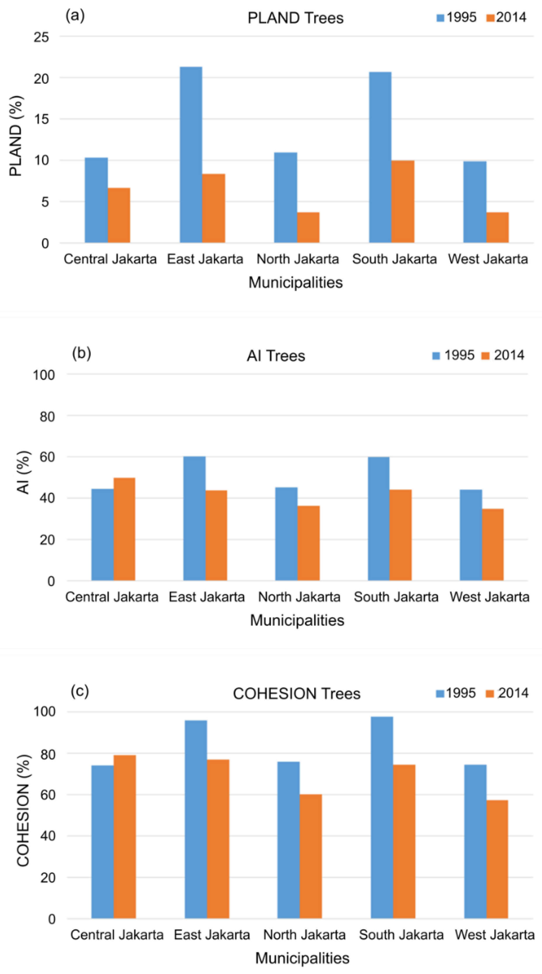
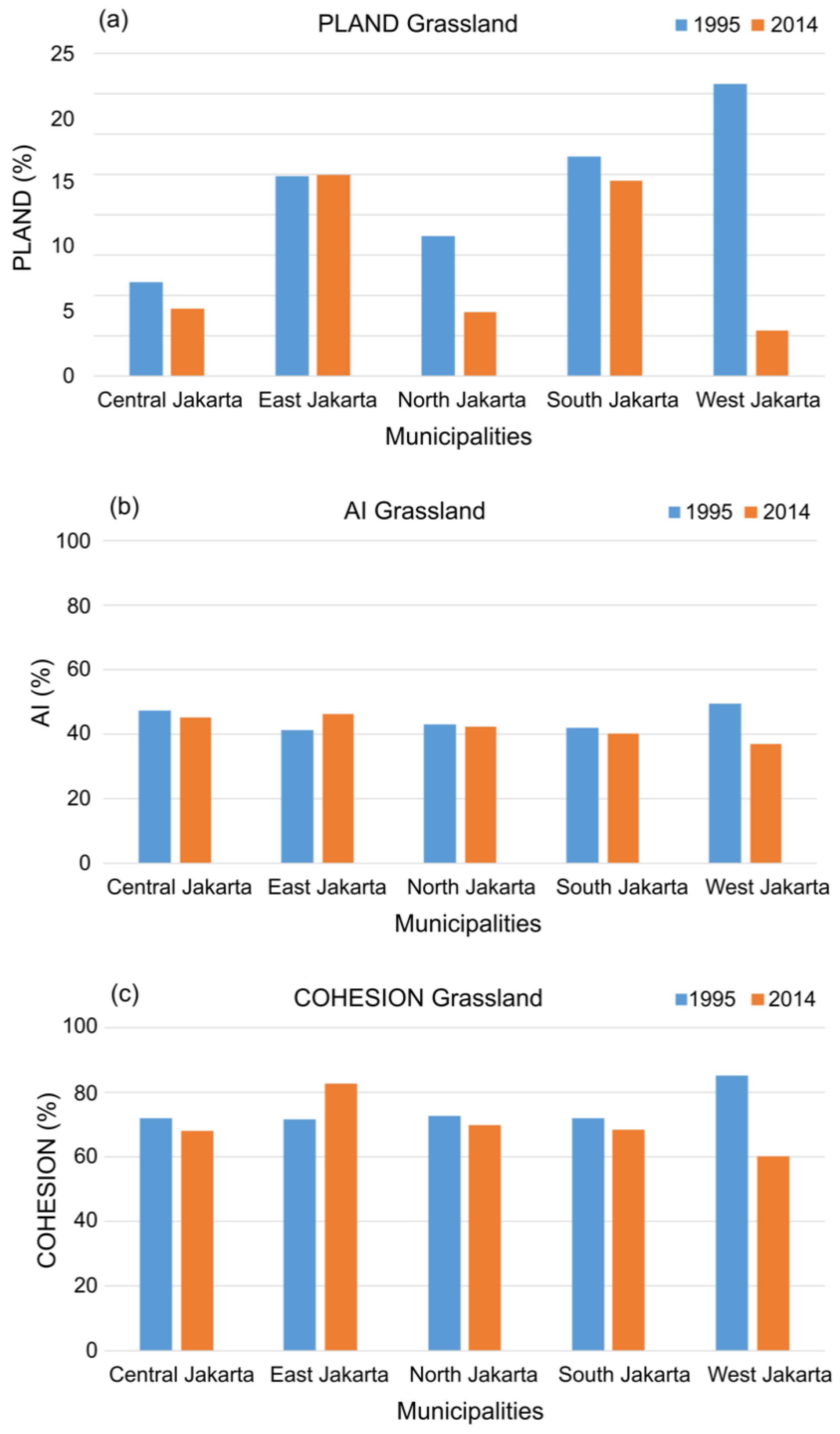
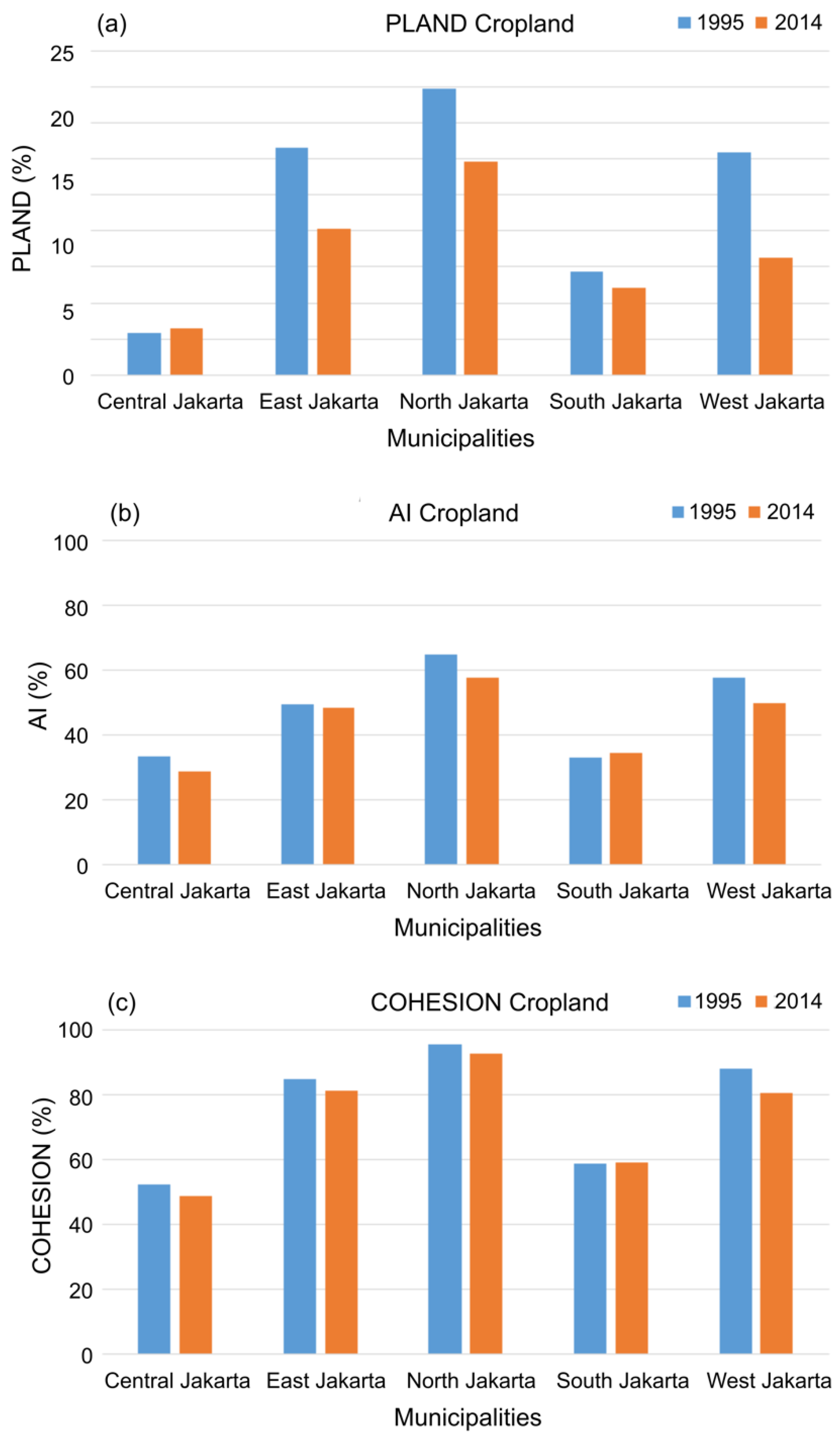
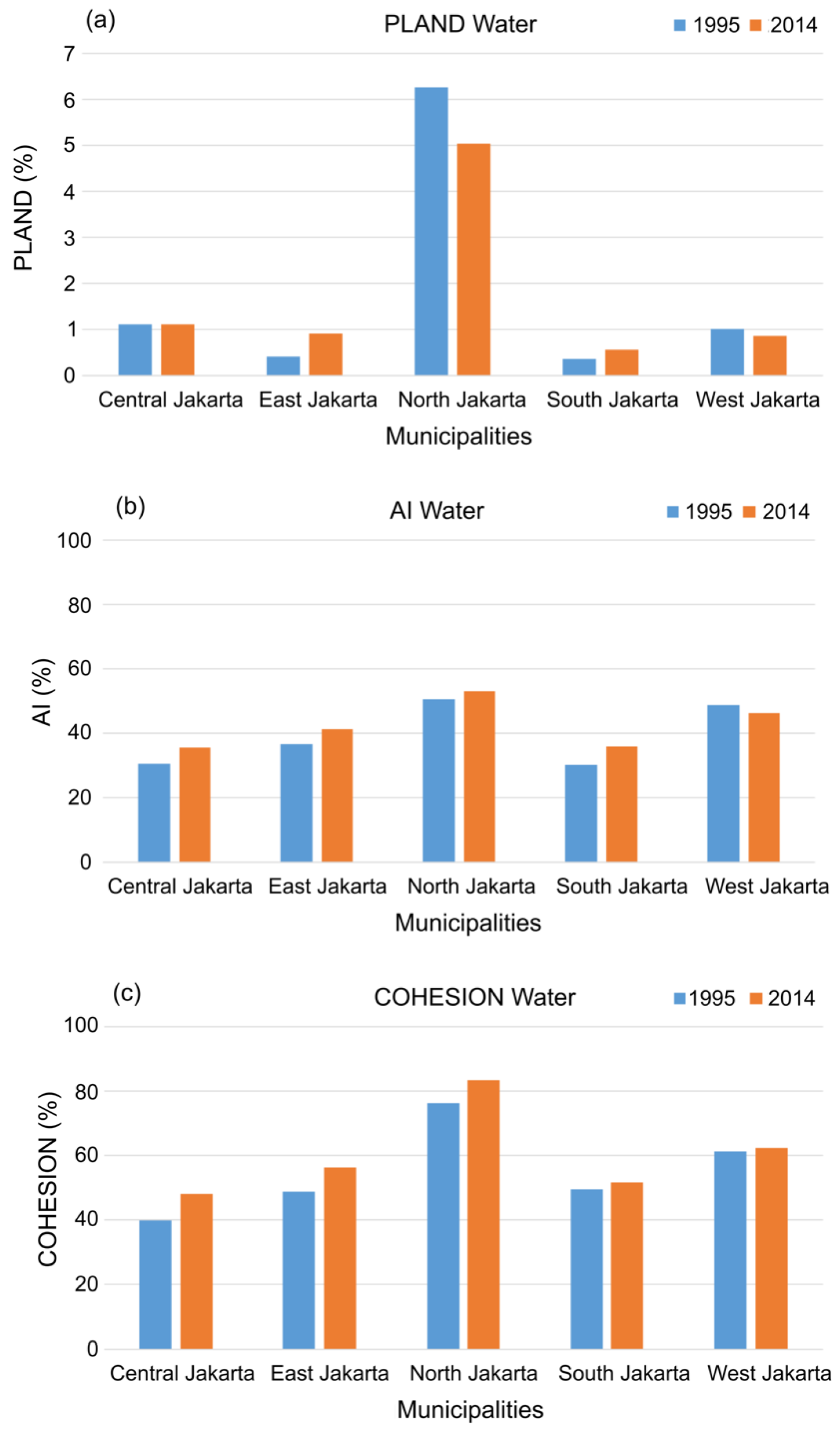
3.2. Landscape Metrics Analysis

The rapid urbanization in Jakarta not only changed the spatial distribution of green spaces but also altered the landscape patterns indicated by changes in the proportion, the aggregation, and the connectivity of green spaces, as well as of bodies of water. In 1995, landscape metrics analysis showed the highest proportion of trees at the municipality level of about 20% in East Jakarta and South Jakarta, while other municipalities had about 10% of trees in their area. Meanwhile, trees showed a dispersed distribution in Central Jakarta, North Jakarta, and West Jakarta, where the AI was lower than 50%. However, trees had good connectivity, as shown in Figure 6. It shows that trees had the COHESION higher than 60% in all municipalities, with the highest values being observed in South Jakarta.

In 2014, the proportion of trees decreased in all municipalities, where the highest decrease of 65.8% was observed in North Jakarta, followed by West Jakarta and East Jakarta, where the proportion decreased by 62.2 and 61.1%, respectively. Meanwhile, the highest trees proportion of 9.9% was identified in South Jakarta, followed by East Jakarta (8.3%) and Central Jakarta (6.6%), while a similar proportion was observed in West Jakarta and North Jakarta. The decrease in the proportion of trees was followed by a decrease in the aggregation and the connectivity of trees except in Central Jakarta. It was found that trees in Central Jakarta were more aggregated and connected in a small proportion. The aggregation and the connectivity of trees in Central Jakarta increased by 12.1 and 6.7%, respectively. In other municipalities, trees were more disaggregated, as indicated by a decrease in the AI values. For instance, the AI in East Jakarta and South Jakarta decreased by 27.4 and 26.3%, respectively. Furthermore, the connectivity of trees also decreased in East Jakarta and South Jakarta, where the connectivity decreased by 19.7 and 23.8%, respectively. However, the connectivity of trees was still high in all municipalities since the COHESION was higher than 50%.

Meanwhile, the dominant proportion of the urban areas also influenced the landscape patterns of the grassland, as shown in Figure 7. In 1995, the highest proportion of grassland was about 14.5% in West Jakarta, followed by South Jakarta (10.9%) and East Jakarta (9.9%). The proportion of grassland in West Jakarta was found higher than the proportion of trees in the same year, which showed a different green space pattern in a municipality. Meanwhile, the low AI percentage indicated that grassland had dispersed distribution in all municipalities. The connectivity of grassland in 1995 was almost similar in four municipalities where the connectivity varied from 71.4% to 72.4%. The highest connectivity of grassland was observed in West Jakarta, where COHESION was 84.9%.

In 2014, all municipalities saw a decrease in the proportion of grassland. The highest decrease was observed in West Jakarta, where the proportion decreased from 14.5% in 1995 to 2.2% in 2014. In addition, the location of the highest proportion shifted from West Jakarta to East Jakarta. The highest grassland proportion of 9.9% was identified in East Jakarta, which was slightly higher than 9.6% in South Jakarta. On the other hand, a similarly low proportion was observed in Central Jakarta, North Jakarta, and West Jakarta, where the proportion of grassland was 3.3, 3.2, and 2.2%, respectively. Furthermore, the area of grassland underwent a small amount of disaggregation in all municipalities except in East Jakarta, where the area of grassland was aggregated by 12.7%. The connectivity of grassland in 2014 was also affected by urbanization as it decreased in four municipalities, but it increased in East Jakarta. The highest decrease was 29.3%: this was observed in West Jakarta, where the connectivity reduced from 84.9% in 1995 to 60.0% in 2014. Moreover, a small decrease was found in Central Jakarta, South Jakarta, and North Jakarta, where the connectivity decreased by 5.9, 5.3, and 3.5%, respectively.

Moreover, the landscape patterns of cropland were also subject to dynamic changes due to urbanization, as shown in Figure 8. In 1995, the highest proportion of cropland was mainly observed in North Jakarta, East Jakarta, and West Jakarta. The highest cropland proportion of 15.9% was observed in North Jakarta, while the lowest cropland proportion of 2.3% was observed in Central Jakarta. Meanwhile, the cropland distribution in the four municipalities exhibited a scattered pattern, as indicated by the AI percentage. For instance, cropland in Central Jakarta, East Jakarta, and South Jakarta was below 50%. Moreover, the connectivity of crops was high in North Jakarta, West Jakarta, and East Jakarta, where the COHESION was 95.3, 87.9, and 84.6%, respectively.

In 2014, the proportion of cropland decreased sharply. The highest decrease of 47.1% was identified in West Jakarta, followed by East Jakarta and North Jakarta, where cropland decreased by 35.9 and 25.2%, respectively. However, North Jakarta still had the highest cropland proportion of 11.9%, while the smallest cropland proportion of 2.6% was observed in Central Jakarta. The decrease in the proportion of cropland affected its aggregation in some municipalities in 2014. For instance, cropland in West Jakarta was disaggregated by 13.9%, followed by North Jakarta and Central Jakarta, where cropland was disaggregated by 11.3 and 13.8%, respectively. Furthermore, cropland had a small decrease in the connectivity, but the percentage was still high. For instance, the highest decrease of 8.4% was observed in West Jakarta, where the connectivity of crops was 87.9%.

In contrast with the landscape patterns of green spaces, urbanization did not have a significant impact on the landscape patterns of bodies of water, as depicted in Figure 9. The proportion of bodies of water in 2014 was similar to that in 1995. The dynamic changes of the landscape patterns of bodies of water were marked by a small increase in the proportion of bodies of water in East Jakarta and South Jakarta, while this proportion decreased in North Jakarta and West Jakarta. However, the aggregation and the connectivity of bodies of water increased in all municipalities in 2014, as shown in Figure 9.

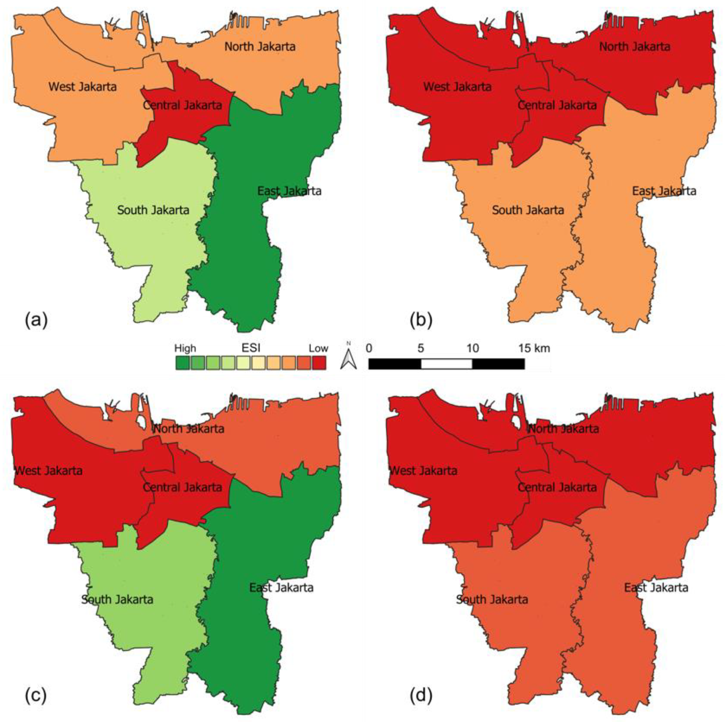
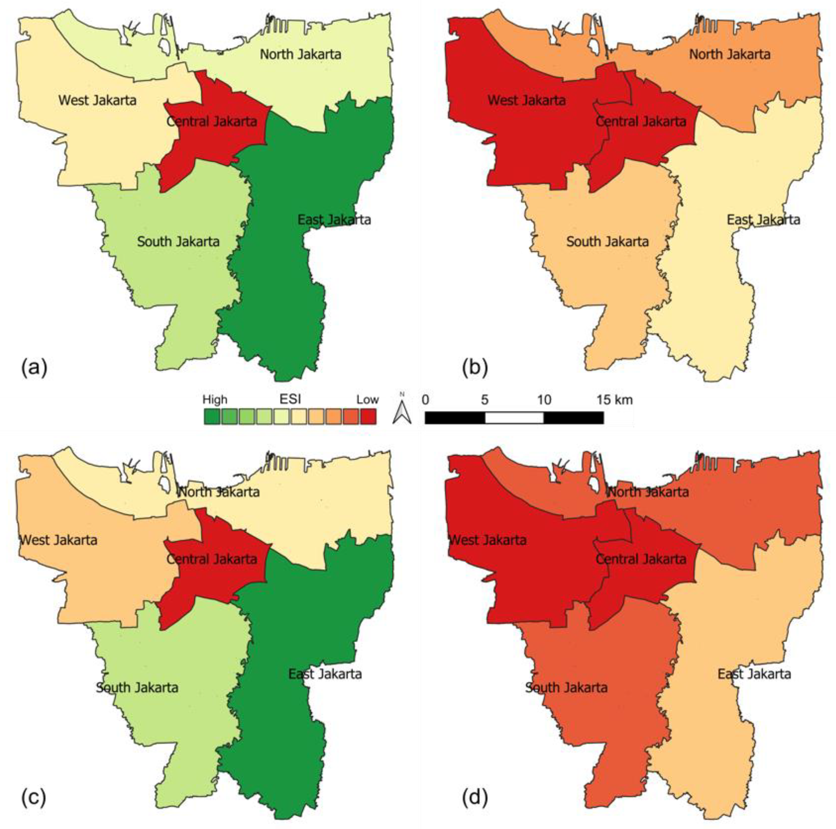
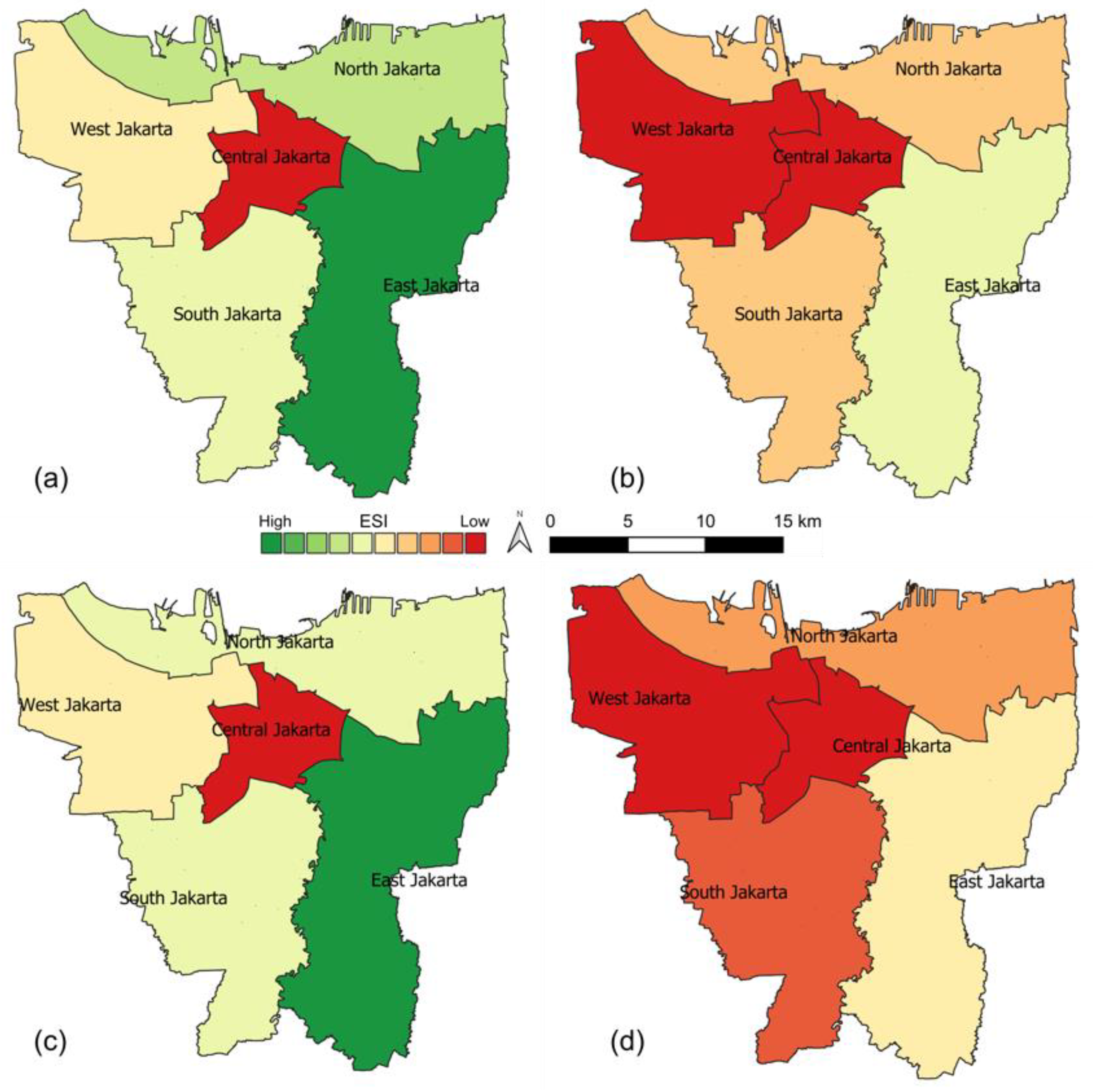
3.3. Spatial and Temporal Distribution of ES Changes

The spatial and temporal distribution of ES changes were analyzed using Equations (2) and (3). The results showed that the landscape pattern changes had a significant impact on the decrease in the carbon sequestration, temperature regulation, and runoff regulation.

The spatiotemporal changes of the carbon sequestration are given in Figure 10. The picture shows that the area-based estimation and the LMA-based estimation give an almost similar pattern of the carbon sequestration, but the decrease rates are different. The area-based estimation that used a lumped area of trees gave a higher carbon sequestration capacity compared to that from the LMA-based estimation, which used an effective area. The area-based estimation showed that East Jakarta had the highest carbon sequestration in 2014, followed by South Jakarta, North Jakarta, West Jakarta, and Central Jakarta. The highest decrease in the carbon sequestration was identified in North Jakarta (−65.8%), followed by West Jakarta (−62.2%), East Jakarta (−61.1%), South Jakarta (−51.8%), and Central Jakarta (−35.5%). On the other hand, the landscape pattern changes in the LMA-based estimation gave a significant change in the carbon sequestration capacity. For instance, the LMA-based estimation suggested that North Jakarta had the highest decrease in the carbon sequestration (−78.4%), followed by East Jakarta (−77.3%), West Jakarta (−77.1%), South Jakarta (72.9%), and Central Jakarta (−22.8%). Furthermore, East Jakarta had the highest carbon sequestration in 2014, followed by South Jakarta, Central Jakarta, North Jakarta, and West Jakarta.

The different spatial patterns of the temperature regulation indicate the influence of the landscape patterns of green spaces and bodies of water, as shown in Figure 11. It shows that the temperature regulation from the LMA-based estimation had a higher decrease rate compared to that from the area-based estimation. The impact of the landscape pattern changes on the temperature regulation was reflected in the LMA-based estimation that suggested the highest decrease rate in West Jakarta (−74.6%), followed by South Jakarta (−64.1%), East Jakarta (−61.1%), North Jakarta (−50.1%), and Central Jakarta (−23.7%). Moreover, the highest temperature regulation in 2014 was in East Jakarta, followed by North Jakarta, South Jakarta, West Jakarta, and Central Jakarta. On the other hand, the area-based estimation showed a similar spatial distribution of the temperature regulation, but the decrease rate was lower than that in the LMA-based estimation. For instance, the decrease rate of the temperature regulation with the area-based estimation in East Jakarta was −44.7% lower than that from the LMA-based estimation. This decreased pattern was also observed in all municipalities.

Furthermore, the dynamic changes of the landscape patterns affect the spatial distribution of the runoff regulation, as shown in Figure 12. It shows that the area-based estimation indicated a decrease of the runoff regulation between 1995 and 2014 in all municipalities where the highest decrease was found in West Jakarta (−64.6%), followed by North Jakarta (−40.5%), East Jakarta (−38.4%), South Jakarta (−33.6%), and Central Jakarta (−25.8%). Meanwhile, East Jakarta had the highest runoff regulation in 2014, followed by South Jakarta and North Jakarta, while the lowest runoff regulation was in Central Jakarta. The LMA-based estimation, on the other hand, showed a higher decrease rate of the runoff regulation. By considering landscape metrics in the effective area of green spaces, the LMA-based estimation suggested that the highest decrease rate was in West Jakarta (−74.6%), followed by South Jakarta (−57.9%), East Jakarta (−51.8%), North Jakarta (−46.3%), and Central Jakarta (−25.0%). Furthermore, the highest runoff regulation was in East Jakarta, followed by North, South Jakarta, West Jakarta, and Central Jakarta.

4. Discussion

4.1. Landscape Pattern Changes and Ecosystem Services

The LULC change analysis shows a considerable change in the spatial distribution and the landscape patterns of green spaces between 1995 and 2014, which in turn affect ecosystem services, as given by the LMA-based estimation. An increase in built-up areas results in a decrease in the size and the proportion of green spaces, as well as in the disaggregation and disconnection of green spaces. A change in the landscape patterns affects the capacity of green spaces to provide ecosystem services [8,45].

This study indicates that the decrease in the carbon sequestration between 1995 and 2014 was influenced by a decrease in the area of green spaces, as well as a decrease in the aggregation and the connectivity of trees. For instance, Central Jakarta was covered with about 3.2 km² of trees in 2014, which is smaller than the area of trees in North Jakarta (namely 5.2 km²). However, the carbon sequestration capacity in Central Jakarta is higher than that in North Jakarta, which can be explained by differences in the landscape patterns. In Central Jakarta, the trees are more aggregated, as indicated by 49.6% of the AI index, while the AI of the trees in North Jakarta is 36.1%. Moreover, the trees in Central Jakarta are more connected, as seen from 78.9% of the COHESION, which is higher than 59.9% in North Jakarta. However, the influence of the connectivity and the aggregation of the trees is not always significant compared to its area. For instance, Central Jakarta has a smaller area and higher connectivity of trees, but carbon sequestration in that area is lower than that in East Jakarta, which has a higher area of trees. Furthermore, the aggregation of trees in East Jakarta is slightly lower than that in Central Jakarta and South Jakarta. The relationship between the carbon sequestration with the area and the landscape patterns of the green spaces is consistent with a previous study in Jakarta, which showed that a higher carbon sequestration rate was observed in the location of a large area of trees [73]. The essential influence of the area of trees in the carbon sequestration was also observed in tropical cities such as Singapore [53] and in cities at high latitudes such as in Espoo, Southern Finland [70]. Moreover, it is important to underline that the carbon sequestration discussed in this study and the examples from other cities are limited to a city or an urban scale. The urban carbon sequestration may not give a significant contribution to the global carbon sequestration process because the total carbon uptake from urban vegetation is smaller than carbon emissions in urban areas, as reported in some cities, including Mexico City and Singapore [92], Beijing [93], and Cebu City, Philippines [94].

The significant influence of the landscape patterns on ecosystem services is also observed when comparing the temperature regulation estimates based on the area and the landscape patterns of green spaces, and bodies of water. Between 1995 and 2014, temperature regulation was found to decrease in all municipalities where the contribution of green spaces is more significant than that of bodies of water, which have small areas and proportions as a result of the land cover classification. As a result, the bodies of water in this study only provide a small contribution to temperature regulation as well as to other ES. Moreover, temperature regulation is more influenced by the area of green spaces than by their connectivity. For instance, the lowest temperature regulation is identified in Central Jakarta and West Jakarta, where the area of green spaces was small in 2014, while the connectivity is high. On the other hand, the highest temperature regulation in 2014 was observed in East Jakarta, where the large area and the high connectivity of green spaces are observed. In addition, the proportion of green spaces in this municipality was relatively higher than that in other municipalities except for West Jakarta. A positive relationship between the increasing urban temperature and the dynamic changes of the landscape patterns has been found in this study which is consistent with the spatial distribution of LST and air temperature in Jakarta discussed in Ramdhoni and Rushayati [37]. In their study, the high LST (higher than 30 °C) was distributed in all municipalities. At the same time, the high air temperature was identified in Central Jakarta, East Jakarta, and North Jakarta, mainly where the small and the fragmented green spaces are observed in our study. The relationship between LST and the landscape patterns of green spaces was also observed in three megacities in Southeast Asia: Jakarta, Bangkok, and Manila [54]. It revealed that Jakarta had the highest mean LST of the three cities considered. It was concluded that this high LST was caused by the relatively large, complex, and more aggregated impervious built-up areas of Jakarta. Furthermore, the impact of the decreasing aggregation and connectivity of green spaces was also identified in the urban center of the Olympic Forest Park in Beijing, China. The observed increase in LST correlated with an increase in the green space fragmentation and a decrease in the green space connectivity [31].

Urbanization in Jakarta between 1995 and 2014 decreased runoff regulation in all municipalities, which could be related to a decrease in green spaces and bodies of water, and the landscape pattern changes. The changes in the runoff regulation are mainly influenced by the dynamic changes of the area and the landscape patterns of green spaces, while the influence of bodies of water is relatively small. The most significant decrease in runoff regulation is observed in West Jakarta, where there has been a high decrease in the area and the proportion of green spaces, which mean West Jakarta has the lowest runoff regulation. Furthermore, in all municipalities the connectivity of green spaces is relatively high while the proportion of green spaces is relatively low and more disaggregated, as shown by a decrease in the aggregation index. The low surface runoff regulation in North Jakarta and West Jakarta is consistent with the area inundated by the 2013 flood [95]. Moreover, the capacity of green spaces to control surface runoff can also be influenced by local physical characteristics such as the slope of the land. However, these characteristics have not been addressed in this study. Increasing the area of green spaces for surface runoff control can be considered in the gentlest sloping area with the high topographic wetness index (TWI), while this is not an appropriate solution in an area with the steep slope and the low TWI [96]. The capacity of green spaces to minimize surface runoff is also associated with LPI and AI. In Beijing, for instance, a decrease of LPI and AI reduced the runoff reduction capacity from 23% in 2000 to 17% in 2010 [30]. The low connectivity and aggregation could be associated with a decrease in the capacity of green spaces to minimize surface runoff. A study from Texas, US, showed that large area, less fragmentation, and high connectivity of green spaces could play an important role in anticipating the mean annual peak runoff. On the other hand, urban development could increase the built-up land cover class, which has more edges, more complex shapes, and is more connected, which facilitates high runoff [97].

4.2. Limitations of This Study and Future Perspectives

The spatial analysis in this study used a medium satellite image resolution of 30 m from Landsat 5 and 8 to analyze three ecosystem services: carbon sequestration, temperature regulation, and runoff regulation. The Landsat products provide a cost-effective option for spatial analysis purposes, such as the LULC change analysis and the landscape metrics analysis. However, some specific urban details such as city parks, small wetland areas, and lakes, as well as street corridors, could not be captured properly. Meanwhile, this study’s results have not yet been validated, which could limit the applicability of the proposed method. Even though it indicates a more realistic ES calculation, the proposed method could potentially bias the results due to different spatial scales used in this study and field survey data.

In future studies, the use of high spatial resolution satellite images for land use–land cover classification is recommended. This increases the spatial analysis quality, and it allows researchers to include more aspects of ecosystem services analysis, such as air purification from trees on street corridors or tourism and educational ecosystem services from the city and the neighborhood parks. The proposed ES estimation could be further improved in the future by incorporating empirical values based on runoff coefficients derived from land cover classes. For validation purposes, future studies should consider methods which apply remote sensing techniques using a range of spatial resolutions combined with actual land management information to identify carbon sequestration rates, land surface temperatures, and flood-prone areas.

5. Conclusions

The present study shows that the landscape pattern changes in the period 1995–2014 have a significant impact on urban ES in Jakarta. The observed landscape pattern changes reduce the carbon sequestration, the temperature regulation, and the runoff regulation with an average value of 66, 55, and 51%, respectively, during that period. The impact of the landscape pattern changes on a decrease of ES is higher compared to the area-based calculation in which the average decrease of the carbon sequestration is 55%, followed by the temperature regulation (44%) and the runoff regulation (41%). This indicates that the ability of green spaces to provide ES is strongly influenced by the spatial characteristics or the landscape patterns of green spaces.

From 1995 to 2014, it is observed that urbanization has not only reduced the number and total surface area of green spaces but also has changed its spatial characteristics. After 20 years, an increase in built-up areas has affected the spatial characteristics of green spaces marked by a scattered distribution, and a decrease in the aggregation and the connectivity of green spaces, making green spaces more fragmented. The average decrease in aggregation is about 8.7 and 9.6% for its connectivity, which can be associated with a decrease in urban ES. The reduced number and area of green spaces along with the landscape pattern changes and a decrease in urban ES indicate that there is a relationship between those factors, which need to be considered as part of the ES calculation.

This study proposes a new method for ES calculation that explicitly acknowledges the landscape patterns of green spaces resulting in the landscape metric area (LMA) of an urban area. The LMA reflects the area which is defined as green space that provides an effective contribution to ES. The spatial characteristics of green spaces are not static, but change over time. This study has shown that urbanization is a factor that impacts the separation and disaggregation as well as the disconnection of green spaces—and thus to a large extent the spatial distribution of green spaces. Ignoring the influence of the landscape patterns may result in an overestimation of the ES of an urban area, as shown in this study.

The importance of the area of green spaces to ES provision has been discussed in many previous studies, which feed the general perception that there is a positive relationship between the area of green spaces and ES. The findings of our study contribute to the existing body of knowledge in this field and suggest that ES calculations should consider not only the area of green spaces but also the landscape patterns, which represent the spatial configuration of green spaces. By considering the landscape patterns in this study, the proposed method indicates a more realistic ES calculation compared to commonly area-based approaches in which green spaces can be perceived as a lumped area. Our study is one of the first to provide quantified and convincing evidence of the influence of the landscape pattern changes on urban ecosystem services in a megacity such as Jakarta. We acknowledge that further detailed studies will be needed and that the present study will provide incentives and directions to initiate further research. It is recommended to further improve this new method by using land cover classification from a high satellite image resolution, considering more landscape metric combinations, incorporating empirical values such as runoff coefficients or albedo values based on LULC, using field survey data or using model simulations to verify the ES calculation.

References

1. United Nations Trends in Urbanization. In World Urbanization Prospects; United Nations: New York, NY, USA, 2014; Volume 12, pp. 7–12. ISBN 9789211515176.
2. Dou, Y.; Kuang, W. A comparative analysis of urban impervious surface and green space and their dynamics among 318 different size cities in China in the past 25 years. Sci. Total Environ. 2020, 706, 135828. [Google Scholar] [CrossRef]
3. Wu, Y.; Tao, Y.; Yang, G.; Ou, W.; Pueppke, S.; Sun, X.; Chen, G.; Tao, Q. Impact of land use change on multiple ecosystem services in the rapidly urbanizing Kunshan City of China: Past trajectories and future projections. Land Use Policy 2019, 85, 419–427. [Google Scholar] [CrossRef]
4. Xu, Q.; Dong, Y.-X.; Yang, R. Influence of land urbanization on carbon sequestration of urban vegetation: A temporal cooperativity analysis in Guangzhou as an example. Sci. Total Environ. 2018, 635, 26–34. [Google Scholar] [CrossRef] [PubMed]
5. Ye, Y.; Bryan, B.A.; Zhang, J.; Connor, J.D.; Chen, L.; Qin, Z.; He, M. Changes in land-use and ecosystem services in the Guangzhou-Foshan Metropolitan Area, China from 1990 to 2010: Implications for sustainability under rapid urbanization. Ecol. Indic. 2018, 93, 930–941. [Google Scholar] [CrossRef]
6. Alcamo, J.; Ash, N.J.; Butler, C.D.; Callicot, J.B.; Capistrano, D.; Carpenter, S.R.; Castilla, J.C.; Chambers, R.; Chopta, K.; Cropper, A.; et al. Ecosystem and Their Services. In Ecosystems and Human Well-Being: A Framework for Assessment; Reid, W.V., Ed.; Island Press: Washington, DC, USA, 2003; pp. 49–70. ISBN 1559634022. [Google Scholar]
7. Bolund, P.; Hunhammar, S. Ecosystem services in urban areas. Ecol. Econ. 1999, 29, 293–301. [Google Scholar] [CrossRef]
8. Burkhard, B.; Kroll, F.; Nedkov, S.; Müller, F. Mapping ecosystem service supply, demand and budgets. Ecol. Indic. 2012, 21 (Suppl. C), 17–29. [Google Scholar] [CrossRef]
9. Derkzen, M.L.; Van Teeffelen, A.J.A.; Verburg, P.H. REVIEW: Quantifying urban ecosystem services based on high-resolution data of urban green space: An assessment for Rotterdam, the Netherlands. J. Appl. Ecol. 2015, 52, 1020–1032. [Google Scholar] [CrossRef]
10. Gkatsopoulos, P. A Methodology for Calculating Cooling from Vegetation Evapotranspiration for Use in Urban Space Microclimate Simulations. Procedia Environ. Sci. 2017, 38, 477–484. [Google Scholar] [CrossRef]
11. Gómez-Baggethun, E.; Barton, D.N. Classifying and valuing ecosystem services for urban planning. Ecol. Econ. 2013, 86, 235–245. [Google Scholar] [CrossRef]
12. Tratalos, J.; Fuller, R.A.; Warren, P.H.; Davies, R.G.; Gaston, K.J. Urban form, biodiversity potential and ecosystem services. Landsc. Urban Plan. 2007, 83, 308–317. [Google Scholar] [CrossRef]
13. Van Oudenhoven, A.P.E.; Petz, K.; Alkemade, R.; Hein, L.; De Groot, R.S. Framework for systematic indicator selection to assess effects of land management on ecosystem services. Ecol. Indic. 2012, 21, 110–122. [Google Scholar] [CrossRef]
14. Panagopoulos, T.; Duque, J.A.G.; Dan, M.B. Urban planning with respect to environmental quality and human well-being. Environ. Pollut. 2016, 208, 137–144. [Google Scholar] [CrossRef] [PubMed] [Green Version]
15. Loures, L.; Santos, R.; Panagopoulos, T. Urban parks and sustainable city planning—The case of Portimão, Portugal. Population 2007, 15, 171–180. [Google Scholar]
16. Clerici, N.; Cote-Navarro, F.; Escobedo, F.J.; Rubiano, K.; Villegas, J.C. Spatio-temporal and cumulative effects of land use-land cover and climate change on two ecosystem services in the Colombian Andes. Sci. Total Environ. 2019, 685, 1181–1192. [Google Scholar] [CrossRef] [PubMed]
17. Depietri, Y.; Renaud, F.G.; Kallis, G. Heat waves and floods in urban areas: A policy-oriented review of ecosystem services. Sustain. Sci. 2011, 7, 95–107. [Google Scholar] [CrossRef]
18. Dupras, J.; Marull, J.; Parcerisas, L.; Coll, F.; Gonzalez, A.; Girard, M.; Tello, E. The impacts of urban sprawl on ecological connectivity in the Montreal Metropolitan Region. Environ. Sci. Policy 2016, 58, 61–73. [Google Scholar] [CrossRef] [Green Version]
19. Fox, D.M.; Witz, E.; Blanc, V.; Soulié, C.; Penalver-Navarro, M.; Dervieux, A. A case study of land cover change (1950–2003) and runoff in a Mediterranean catchment. Appl. Geogr. 2012, 32, 810–821. [Google Scholar] [CrossRef]
20. Farrugia, S.; Hudson, M.D.; McCulloch, L. An evaluation of flood control and urban cooling ecosystem services delivered by urban green infrastructure. Int. J. Biodivers. Sci. Ecosyst. Serv. Manag. 2012, 9, 136–145. [Google Scholar] [CrossRef]
21. Marando, F.; Salvatori, E.; Sebastiani, A.; Fusaro, L.; Manes, F. Regulating Ecosystem Services and Green Infrastructure: Assessment of Urban Heat Island effect mitigation in the municipality of Rome, Italy. Ecol. Model. 2019, 392, 92–102. [Google Scholar] [CrossRef]
22. Yuan, Y.; Wu, S.; Yu, Y.; Tong, G.; Mo, L.; Yan, D.; Li, F. Spatiotemporal interaction between ecosystem services and urbanization: Case study of Nanjing City, China. Ecol. Indic. 2018, 95, 917–929. [Google Scholar] [CrossRef]
23. Jaligot, R.; Kemajou, A.; Chenal, J. Cultural ecosystem services provision in response to urbanization in Cameroon. Land Use Policy 2018, 79, 641–649. [Google Scholar] [CrossRef]
24. Das, M.; Das, A. Dynamics of Urbanization and its impact on Urban Ecosystem Services (UESs): A study of a medium size town of West Bengal, Eastern India. J. Urban Manag. 2019, 8, 420–434. [Google Scholar] [CrossRef]
25. Costanza, R.; d’Arge, R.; de Groot, R.; Farber, S.; Grasso, M.; Hannon, B.; Limburg, K.; Naeem, S.; O’Neill, R.V.; Paruelo, J.; et al. The value of the world’s ecosystem services and natural capital. Nature 1997, 387, 253–260. [Google Scholar] [CrossRef]
26. Wang, J.; Zhou, W.; Pickett, S.T.; Yu, W.; Li, W. A multiscale analysis of urbanization effects on ecosystem services supply in an urban megaregion. Sci. Total Environ. 2019, 662, 824–833. [Google Scholar] [CrossRef] [PubMed]
27. Asadolahi, Z.; Salmanmahiny, A.; Sakieh, Y.; Mirkarimi, S.H.; Baral, H.; Azimi, M. Dynamic trade-off analysis of multiple ecosystem services under land use change scenarios: Towards putting ecosystem services into planning in Iran. Ecol. Complex. 2018, 36, 250–260. [Google Scholar] [CrossRef]
28. Haas, J.; Furberg, D.; Ban, Y. Satellite monitoring of urbanization and environmental impacts—A comparison of Stockholm and Shanghai. Int. J. Appl. Earth Obs. Geoinf. 2015, 38, 138–149. [Google Scholar] [CrossRef]
29. Bai, T.; Mayer, A.L.; Shuster, W.D.; Tian, G. The Hydrologic Role of Urban Green Space in Mitigating Flooding (Luohe, China). Sustainability 2018, 10, 3584. [Google Scholar] [CrossRef] [Green Version]
30. Zhang, B.; Xie, G.-D.; Li, N.; Wang, S. Effect of urban green space changes on the role of rainwater runoff reduction in Beijing, China. Landsc. Urban Plan. 2015, 140, 8–16. [Google Scholar] [CrossRef]
31. Amani-Beni, M.; Zhang, B.; Xie, G.-D.; Shi, Y. Impacts of Urban Green Landscape Patterns on Land Surface Temperature: Evidence from the Adjacent Area of Olympic Forest Park of Beijing, China. Sustainability 2019, 11, 513. [Google Scholar] [CrossRef] [Green Version]
32. Jaganmohan, M.; Knapp, S.; Buchmann, C.M.; Schwarz, N. The Bigger, the Better? The Influence of Urban Green Space Design on Cooling Effects for Residential Areas. J. Environ. Qual. 2016, 45, 134–145. [Google Scholar] [CrossRef] [PubMed]
33. Mitchell, M.G.; Suarez-Castro, A.F.; Martinez-Harms, M.; Maron, M.; McAlpine, C.; Gaston, K.J.; Johansen, K.; Rhodes, J.R. Reframing landscape fragmentation’s effects on ecosystem services. Trends Ecol. Evol. 2015, 30, 190–198. [Google Scholar] [CrossRef] [PubMed] [Green Version]
34. Mitchell, M.G.E.; Bennett, E.M.; Gonzalez, A. Linking Landscape Connectivity and Ecosystem Service Provision: Current Knowledge and Research Gaps. Ecosystems 2013, 16, 894–908. [Google Scholar] [CrossRef]
35. Nagasawa, R.; Fukushima, A.; Yayusman, L.F.; Novresiandi, D.A. Urban Expansion and Its Influences on The Suburban Land Use Change in Jakarta Metropolitan Region (JABODETABEK). Urban Plan. Des. Res. 2015, 3, 7. [Google Scholar] [CrossRef]
36. Pravitasari, A.E. Study on Impact of Urbanization and Rapid Urban Expansion in Java and Jabodetabek, Megacity in Indonesia; Kyoto University: Kyoto, Japan, 2015. [Google Scholar]
37. Ramdhoni, S.; Rushayati, S.B.; Prasetyo, L.B. Open Green Space Development Priority Based on Distribution of air Temperature Change in Capital City of Indonesia, Jakarta. Procedia Environ. Sci. 2016, 33, 204–213. [Google Scholar] [CrossRef] [Green Version]
38. Rustiadi, E.; Zain, A.M.; Trisasongko, B.H.; Carolita, I. Land Cover Change in Jabotabek Region; Himiyama, Y., Mather, A., Bicik, I., Milanova, E.V., Eds.; International Geographical Union Commission on Land Use/Cover Change: Hokkaido, Japan, 2002. [Google Scholar]
39. Firman, T. The continuity and change in mega-urbanization in Indonesia: A survey of Jakarta–Bandung Region (JBR) development. Habitat Int. 2009, 33, 327–339. [Google Scholar] [CrossRef]
40. BPS DKI Jakarta Jakarta in Figures 2016; BPS Provinsi DKI Jakarta/Jakarta Statistics Bureau: Jakarta, Indonesia, 2016.
41. De Ridder, K.; Adamec, V.; Bañuelos, A.; Bruse, M.; Bürger, M.; Damsgaard, O.; Dufek, J.; Hirsch, J.; Lefebre, F.; Pérez-Lacorzana, J.; et al. An integrated methodology to assess the benefits of urban green space. Sci. Total Environ. 2004, 334–335, 489–497. [Google Scholar] [CrossRef]
42. Leroux, L.; Congedo, L.; Bellón, B.; Gaetano, R.; Bégué, A. Land Cover Mapping Using Sentinel-2 Images and the Semi-Automatic Classification Plugin: A Northern Burkina Faso Case Study. In QGIS and Applications in Agriculture and Forest; Wiley: Hoboken, NJ, USA, 2018; pp. 119–151. [Google Scholar]
43. Arowolo, A.O.; Deng, X.; Olatunji, O.A.; Obayelu, A.E. Assessing changes in the value of ecosystem services in response to land-use/land-cover dynamics in Nigeria. Sci. Total Environ. 2018, 636, 597–609. [Google Scholar] [CrossRef] [PubMed]
44. Gökyer, E. Understanding landscape structure using landscape metrics. In Advances in Landscape Architecture; Özyavuz, M., Ed.; IntechOpen: London, UK, 2013. [Google Scholar]
45. Mugiraneza, T.; Ban, Y.; Haas, J. Urban land cover dynamics and their impact on ecosystem services in Kigali, Rwanda using multi-temporal Landsat data. Remote. Sens. Appl. Soc. Environ. 2019, 13, 234–246. [Google Scholar] [CrossRef]
46. Daniels, B.; Zaunbrecher, B.S.; Paas, B.; Ottermanns, R.; Ziefle, M.; Roß-Nickoll, M. Assessment of urban green space structures and their quality from a multidimensional perspective. Sci. Total Environ. 2018, 615, 1364–1378. [Google Scholar] [CrossRef] [PubMed]
47. Estoque, R.C.; Murayama, Y. Landscape pattern and ecosystem service value changes: Implications for environmental sustainability planning for the rapidly urbanizing summer capital of the Philippines. Landsc. Urban Plan. 2013, 116, 60–72. [Google Scholar] [CrossRef]
48. McGarigal, K.; Cushman, S.; Ene, E. FRAGSTATS v4: Spatial Pattern Analysis Program for Categorical and Continuous Maps. Computer Software Program; University of Massachusetts: Amherst, MA, USA; Available online: http://www.umass.edu/landeco/research/fragstats/fragstats.html (accessed on 30 September 2019).
49. De Smith, M.J.; Goodchild, M.F.; Longley, P. Geospatial Analysis: A Comprehensive Guide to Principles, Techniques and Software Tools; Troubador Publishing Ltd.: Leicester, UK, 2007; ISBN 1-905886-60-8. [Google Scholar]
50. Kong, F.; Yin, H.; Nakagoshi, N.; Zong, Y. Urban green space network development for biodiversity conservation: Identification based on graph theory and gravity modeling. Landsc. Urban Plan. 2010, 95, 16–27. [Google Scholar] [CrossRef]
51. He, H.S.; Dezonia, B.E.; Mladenoff, D.J. An aggregation index (AI) to quantify spatial patterns of landscapes. Landsc. Ecol. 2000, 15, 591–601. [Google Scholar] [CrossRef]
52. Bao, T.; Li, X.; Zhang, J.; Zhang, Y.; Tian, S. Assessing the Distribution of Urban Green Spaces and its Anisotropic Cooling Distance on Urban Heat Island Pattern in Baotou, China. ISPRS Int. J. Geo-Inf. 2016, 5, 12. [Google Scholar] [CrossRef]
53. Chen, J.; Goh, J. Carbon Accounting in Local-Scale Land Use and Land Cover Change. Cons. J. Sustaianble Dev. 2017, 17, 46–74. [Google Scholar]
54. Estoque, R.C.; Murayama, Y.; Myint, S.W. Effects of landscape composition and pattern on land surface temperature: An urban heat island study in the megacities of Southeast Asia. Sci. Total Environ. 2017, 577, 349–359. [Google Scholar] [CrossRef] [PubMed]
55. Li, X.; Zhou, W.; Ouyang, Z.; Xu, W.; Zheng, H. Spatial pattern of greenspace affects land surface temperature: Evidence from the heavily urbanized Beijing metropolitan area, China. Landsc. Ecol. 2012, 27, 887–898. [Google Scholar] [CrossRef]
56. Ramesh, R.; Chen, Z.; Cummins, V.; Day, J.; D’Elia, C.; Dennison, B.; Forbes, D.; Glaeser, B.; Glaser, M.; Glavovic, B.; et al. Land–Ocean Interactions in the Coastal Zone: Past, present & future. Anthropocene 2015, 12, 85–98. [Google Scholar] [CrossRef] [Green Version]
57. Werner, C. Green open spaces in Indonesian cities: Schisms between law and practice. Pacific Geogr. 2014, 41, 26–31. [Google Scholar]
58. Cortinovis, C.; Geneletti, D. Ecosystem services in urban plans: What is there, and what is still needed for better decisions. Land Use Policy 2018, 70, 298–312. [Google Scholar] [CrossRef]
59. Vincent, S.U.; Radhakrishnan, M.; Hayde, L.; Pathirana, A. Enhancing the Economic Value of Large Investments in Sustainable Drainage Systems (SuDS) through Inclusion of Ecosystems Services Benefits. Water 2017, 9, 841. [Google Scholar] [CrossRef] [Green Version]
60. Rotterdam, C. Rotterdam Programme on Sustainability and Climate Change 2015–2018; City of Rotterdam: Rotterdam, The Netherlands, 2015. [Google Scholar]
61. Urban Ecology Programme 2011–2026; Department of Environmental Affairs and Transport: Oslo, Norway, 2011.
62. Environmental Action 2016–2021: Strategy and Action Plan; City of Sydney Council: Sydney, Australia, 2017; Available online: https://apo.org.au/sites/default/files/resource-files/2017-03/apo-nid174586.pdf (accessed on 20 February 2021).
63. Arifin, H.S.; Nakagoshi, N. Landscape ecology and urban biodiversity in tropical Indonesian cities. Landsc. Ecol. Eng. 2011, 7, 33–43. [Google Scholar] [CrossRef]
64. Rusiawan, W.; Tjiptoherijanto, P.; Suganda, E.; Darmajanti, L. System Dynamics Modeling for Urban Economic Growth and CO2 Emissions: A Case Study of Jakarta, Indonesia. Procedia Environ. Sci. 2015, 28, 330–340. [Google Scholar] [CrossRef] [Green Version]
65. Surahman, U.; Kubota, T.; Wijaya, A. Life cycle assessment of energy and CO2emissions for residential buildings in Jakarta, Indonesia. IOP Conf. Ser. Mater. Sci. Eng. 2016, 128, 012002. [Google Scholar] [CrossRef]
66. Siswanto, G.J.; Van Der Schrier, G.; Lenderink, G.; Hurk, B.V.D. Trends in High-Daily Precipitation Events in Jakarta and the Flooding of January. Bull. Am. Meteorol. Soc. 2015, 96, 131–135. [Google Scholar] [CrossRef]
67. Wijayanti, P.; Zhu, X.; Hellegers, P.; Budiyono, Y.; Van Ierland, E.C. Estimation of river flood damages in Jakarta, Indonesia. Nat. Hazards 2017, 86, 1059–1079. [Google Scholar] [CrossRef] [Green Version]
68. Darmanto, N.S.; Varquez, A.C.G.; Kawano, N.; Kanda, M. Future urban climate projection in a tropical megacity based on global climate change and local urbanization scenarios. Urban Clim. 2019, 29, 100482. [Google Scholar] [CrossRef]
69. Churkina, G. Carbon cycle of urban ecosystems. In Carbon Sequestration in Urban Ecosystems; Lal, R., Augustin, B., Eds.; Springer: Berlin/Heidelberg, Germany, 2011; p. 315. ISBN 978-94-007-2365-8. [Google Scholar]
70. Kuittinen, M.; Moinel, C.; Adalgeirsdottir, K. Carbon sequestration through urban ecosystem services. Sci. Total Environ. 2016, 563–564, 623–632. [Google Scholar] [CrossRef]
71. Nero, B.F.; Callo-Concha, D.; Anning, A.; Denich, M. Urban Green Spaces Enhance Climate Change Mitigation in Cities of the Global South: The Case of Kumasi, Ghana. Procedia Eng. 2017, 198, 69–83. [Google Scholar] [CrossRef]
72. Forman, R.T.T. Urban Ecology: Science of Cities; Cambridge University Press: Cambridge, UK, 2014; ISBN 9781139030472. [Google Scholar]
73. Azaria, L.; Wibowo, A.; Shidiq, I.P.A. Rokhmatuloh Carbon Sequestration Capability Analysis of Urban Green Space Using Geospatial Data. E3S Web Conf. 2018, 73, 03009. [Google Scholar] [CrossRef]
74. Oviantari, M.V.; Gunamantha, I.M.; Ristiati, N.P.; Santiasa, I.M.P.A.; Astariani, P.P.Y. Carbon sequestration by above-ground biomass in urban green spaces in Singaraja city. IOP Conf. Ser. Earth Environ. Sci. 2018, 200, 012030. [Google Scholar] [CrossRef] [Green Version]
75. Oke, T.R.; Mills, G.; Christen, A.; Voogt, J.A. Urban Climates; Cambridge University Press: Cambridge, UK, 2017; ISBN 9781139016476. [Google Scholar]
76. Maheng, D.; Ducton, I.; Lauwaet, D.; Zevenbergen, C.; Pathirana, A. The Sensitivity of Urban Heat Island to Urban Green Space—A Model-Based Study of City of Colombo, Sri Lanka. Atmosphere 2019, 10, 151. [Google Scholar] [CrossRef] [Green Version]
77. Sodoudi, S.; Zhang, H.; Chi, X.; Müller, F.; Li, H. The influence of spatial configuration of green areas on microclimate and thermal comfort. Urban For. Urban Green. 2018, 34, 85–96. [Google Scholar] [CrossRef]
78. Amani-Beni, M.; Zhang, B.; Xie, G.-D.; Xu, J. Impact of urban park’s tree, grass and waterbody on microclimate in hot summer days: A case study of Olympic Park in Beijing, China. Urban For. Urban Green. 2018, 32, 1–6. [Google Scholar] [CrossRef]
79. Steeneveld, G.; Koopmans, S.A.; Heusinkveld, B.G.; Theeuwes, N. Refreshing the role of open water surfaces on mitigating the maximum urban heat island effect. Landsc. Urban Plan. 2014, 121, 92–96. [Google Scholar] [CrossRef]
80. Theeuwes, N.E.; Solcerová, A.; Steeneveld, G.J. Modeling the influence of open water surfaces on the summertime temperature and thermal comfort in the city. J. Geophys. Res. Atmos. 2013, 118, 8881–8896. [Google Scholar] [CrossRef] [Green Version]
81. Chen, Y.-C.; Tan, C.-H.; Wei, C.; Su, Z.-W. Cooling Effect of Rivers on Metropolitan Taipei Using Remote Sensing. Int. J. Environ. Res. Public Health 2014, 11, 1195–1210. [Google Scholar] [CrossRef] [PubMed] [Green Version]
82. Gunawardena, K.; Wells, M.; Kershaw, T. Utilising green and bluespace to mitigate urban heat island intensity. Sci. Total Environ. 2017, 584, 1040–1055. [Google Scholar] [CrossRef]
83. Alves, A.; Vojinovic, Z.; Kapelan, Z.; Sanchez, A.; Gersonius, B. Exploring trade-offs among the multiple benefits of green-blue-grey infrastructure for urban flood mitigation. Sci. Total Environ. 2020, 703, 134980. [Google Scholar] [CrossRef] [PubMed]
84. Yang, B.; Lee, D.K.; Heo, H.K.; Biging, G. The effects of tree characteristics on rainfall interception in urban areas. Landsc. Ecol. Eng. 2019, 15, 289–296. [Google Scholar] [CrossRef] [Green Version]
85. Yao, L.; Chen, L.; Wei, W.; Sun, R. Potential reduction in urban runoff by green spaces in Beijing: A scenario analysis. Urban For. Urban Green. 2015, 14, 300–308. [Google Scholar] [CrossRef]
86. ASCE Hydrology Handbook (Manual N0. 28), 2nd ed.; American Society of Civil Engineers: New York, NY, USA, 1996; ISBN 978-0-7844-0138-5.
87. Alves, P.L.; Formiga, K.T.M.; Traldi, M.A.B. Rainfall interception capacity of tree species used in urban afforestation. Urban Ecosyst. 2018, 21, 697–706. [Google Scholar] [CrossRef]
88. Highfield, W.E. Section 404 Permitting in Coastal Texas: A Longitudinal Analysis of the Relationship Between Peak Streamflow and Wetland Alteration. Environ. Manag. 2012, 49, 892–901. [Google Scholar] [CrossRef]
89. Te Chow, V.; Maidment, D.R.; Mays, L.W. Applied Hydrology; McGraw-Hill Series in Water Resources and Environmental Engineering; McGraw-Hill: Singapore, 1988; ISBN 0070108102. [Google Scholar]
90. Yang, X.; You, X.-Y.; Ji, M.; Nima, C. Influence factors and prediction of stormwater runoff of urban green space in Tianjin, China: Laboratory experiment and quantitative theory model. Water Sci. Technol. 2013, 67, 869–876. [Google Scholar] [CrossRef] [PubMed]
91. Shang, H.; Zhang, K.; Wang, Z.; Yang, J.; He, M.; Pan, X.; Fang, C. Effect of varying wheatgrass density on resistance to overland flow. J. Hydrol. 2020, 591, 125594. [Google Scholar] [CrossRef]
92. Velasco, E.; Roth, M.; Norford, L.; Molina, L.T. Does urban vegetation enhance carbon sequestration? Landsc. Urban Plan. 2016, 148, 99–107. [Google Scholar] [CrossRef]
93. Zhao, S.; Tang, Y.; Chen, A. Carbon Storage and Sequestration of Urban Street Trees in Beijing, China. Front. Ecol. Evol. 2016, 4, 1–8. [Google Scholar] [CrossRef] [Green Version]
94. Pansit, N.R. Carbon storage and sequestration potential of urban trees in Cebu City, Philippines. Mindanao J. Sci. Technol. 2019, 17, 98–111. [Google Scholar]
95. Padawangi, R.; Douglass, M. Water, Water Everywhere: Toward Participatory Solutions to Chronic Urban Flooding in Jakarta. Pac. Aff. 2015, 88, 517–550. [Google Scholar] [CrossRef]
96. Kim, H.; Lee, D.-K.; Sung, S. Effect of Urban Green Spaces and Flooded Area Type on Flooding Probability. Sustainability 2016, 8, 134. [Google Scholar] [CrossRef] [Green Version]
97. Kim, H.W.; Park, Y. Urban green infrastructure and local flooding: The impact of landscape patterns on peak runoff in four Texas MSAs. Appl. Geogr. 2016, 77, 72–81. [Google Scholar] [CrossRef]
Figure 1. Schematic illustration of the loss of information due to lumping green areas. (a) Real landscape pattern; (b) the lumped area used in many previous ecosystem services (ES) studies.
Land 10 00218 g001
Figure 2. (a) Map of Indonesia; (b) Jakarta is located on Java island, which is the densest island in Indonesia; (c) Jakarta consists of five municipalities.
Land 10 00218 g002
Figure 3. Land use–land cover change from 1995 to 2014.
Land 10 00218 g003
Figure 4. The area of land use–land cover of Jakarta in 1995 and 2014. (a) The area of urban class; (b) the area of suburban class; (c) the area of trees; (d) the area of grassland; (e) the area of cropland; (f) the area of bodies of water.
Land 10 00218 g004
Figure 5. The spatial and temporal distribution of green spaces and bodies of water in 1995 and 2014.
Land 10 00218 g005
Figure 6. Landscape metrics of trees. (a) Land proportion; (b) aggregation index; (c) cohesion.
Land 10 00218 g006
Figure 7. Landscape metrics of grassland. (a) Land proportion; (b) aggregation index; (c) cohesion.
Land 10 00218 g007
Figure 8. Landscape metrics of cropland. (a) Land proportion; (b) aggregation index; (c) cohesion.
Land 10 00218 g008
Figure 9. Landscape metrics of water. (a) Land proportion; (b) aggregation index; (c) cohesion.
Land 10 00218 g009
Figure 10. ESI for carbon sequestration in the year 1995 and 2014. (a) ESI in 1995 without LMA; (b) ESI in 2014 without LMA; (c) ESI in 1995 with LMA; and (d) ESI in 2014 with LMA.
Land 10 00218 g010
Figure 11. Ecosystem services index (ESI) for temperature regulation in the year 1995 and 2014. (a) ESI in 1995 without landscape metric area (LMA); (b) ESI in 2014 without LMA; (c) ESI in 1995 with LMA; and (d) ESI in 2014 with LMA.
Land 10 00218 g011
Figure 12. ESI for runoff regulation in the year 1995 and 2014. (a) ESI in 1995 without LMA; (b) ESI in 2014 without LMA; (c) ESI in 1995 with LMA; and (d) ESI in 2014 with LMA.
Land 10 00218 g012