Article

Urban Development and Sustainable Mobility: A Spatial Analysis in the Buenos Aires Metropolitan Area

by
Lorea Mendiola
1,*,† and
Pilar González
2,†
1
Department of Applied Economics I, University of the Basque Country (UPV/EHU), 20018 Donostia-San Sebastian, Spain
2
Department of Quantitative Methods & Institute for Public Economics, University of the Basque Country (UPV/EHU), 48015 Bilbao, Spain
*
Author to whom correspondence should be addressed.
These authors contributed equally to this work.
Land 2021, 10(2), 157; https://doi.org/10.3390/land10020157
Submission received: 8 January 2021 / Revised: 28 January 2021 / Accepted: 1 February 2021 / Published: 4 February 2021

Abstract

:
This study provides empirical evidence on the links between urban development factors and the use of specific modes of transport in commuting in the Buenos Aires metropolitan area. The case study is of interest because quantitative research on developing countries is scarce and their rapid urban growth and high rates of inequality may generate different results compared to the US or Europe. This relationship was assessed on locality level using regression methods. Spatial econometric techniques were applied to avoid unreliable inferences generated by spatial dependence and to detect the existence of externalities. Furthermore, we include in the model the socio-economic profile of each locality identified using cluster analysis. The findings reveal that population density affects motorised transport, that diversity is relevant for public transport and non-motorised trips, and urban design characteristics affect all modes of transport. Spatial dependence is detected for motorised transport, which may imply the existence of externalities, suggesting the need for coordinated decision-making processes on a metropolitan level. Finally, modal split depends on the socio-economic profile of a locality, which may influence the response to public transport policies. To sum up, these results may be useful when it comes to helping policymakers design integrated public policies on urban and transport planning.

1. Introduction

Over the past few decades, cities have been expanding at an unprecedented rate. More than half of the population currently lives in urban areas, and that figure is expected to reach 68.4% by 2050. The most highly urbanised regions are North America, where 82% of the population lives in cities, Latin America and the Caribbean (81%), Europe (74%), and Oceania (68%) [1]. This process of urbanisation has led cities to grow so rapidly that, in many cases, their efforts to provide mobility solutions fail to meet the growing needs of the population. As a result, sustainable mobility has become one of the main challenges in urban life.
The distribution of human activities over urban land creates demand for mobility that is partly met by the transport system. That system, in turn, has significant impacts on shaping future land use patterns. This requires public policies that can organise cities from the dual perspective of mobility demand and transport supply, encouraging the rational use of transport systems in an economically and environmentally sustainable way, solving the serious problems of exclusion and insecurity that currently exist [2]. Most observers agree that, while actions on transport are needed at least in the short and medium run, land use plays an essential role in the long run and this entails designing the composition and densities of land uses in such a way as to reduce the need for travel, shorten journeys, and encourage socially responsible modes of travel [3].
Many empirical studies have analysed and measured the magnitude of the links between urban development factors and mobility with a view to assessing whether the land use policies are valid for managing the demand for mobility. Their findings have allowed us to conclude that, in general, land use factors such as density, functional diversity, and urban design, together with transit and destination accessibility have impacts on modal split [4,5,6,7,8]. However the empirical evidence available to date is sometimes mixed and inconclusive about which factor could be the most influential one [7,9,10], probably due to the different geographical scales, methodologies, and travel features used [5]. In particular, it should be noted that mobility patterns seem to be more strongly associated with diversity, design, and accessibility factors than with population density. The individual impact of each factor may be modest, but cumulatively and synergistically they are relevant when it comes to explaining modal split [5,6].
Empirical research on this topic has been mostly conducted in North America, Europe, and Australia, with far less literature focused on developing countries. Some authors argue that this relationship may be different in these countries [11]. Their specific characteristics such as rapid urbanisation and motorisation, higher rates of poverty and inequality, weaker institutions, and cultural particularities [12,13] lead to different contexts, where the results for western cities may not apply. Most of the research in these countries is concentrated on China, where the urban population has grown at a striking rate in the past few decades, from 26.4% in 1990 to 59.2% in 2018 [9,10,14,15,16,17]. The results obtained for China’s major metropolises are generally similar to those obtained in western research, although Zhang [9] found that density has a stronger relationship with travel behaviour in Boston than in Hong Kong. Even though research is scarce in other developing countries, some studies have been carried out in Bangladesh [18], or the Middle East and North Africa [19].
In the case of Latin America, the analysis of urban mobility has aroused great interest among researchers who have approached it from several viewpoints, but it is still scarce in the specific area of quantifying the relationship between urban development and mobility patterns. Zegras [20] analysed this topic for Santiago de Chile and found that car use depends on distance to transit and intersection density. Guerra et al. [21] studied urban form and commuting in Mexico. Their results show that population density, street density, and transit supply are the urban factors most strongly related to mode choice, with population density playing a particularly strongly role. Both works found that the strength of the relationship between built environment variables, specifically density, and car travel is higher than the average from Ewing’s analysis [5], which consists mainly of studies in the US. With respect to the effects of a built environment on non-motorised travel, Cervero et al. [22] and Rodríguez et al. [23] analysed the case of Bogotá (Colombia). Both studies found that factors such as pedestrian-friendly amenities and connectivity encourage pedestrian activity, while the results are contradictory with respect to land mix uses. By contrast, Larrañaga and Cybis [24] showed that, although land use mix is favourable to walking, socio-economic factors are more important than built environment factors. To sum up, land use affects modal split in commuting but the strength of the effect may differ depending on the socio-cultural realities of each region [25].
The main aim of this paper is to find how and how much different types of urban development (land use factors and public transport characteristics) are related to mobility-to-work patterns on developing countries. Specifically, our study seeks to analyse the link between the urban characteristics of the place of origin of journeys and its mobility pattern, focusing on single-stage commutes from home to work. In addition to this, we propose to test the hypothesis that the link between urban development factors and modal split may vary across socio-economic groups. The case study selected is the Buenos Aires Metropolitan Area (AMBA), a region scarcely studied from a quantitative point of view.
This work contributes to the research field on the relationship between urban development characteristics and modal split in several ways. Firstly, the case study selected. The AMBA is the largest metropolitan area in Argentina, one of the countries with the highest rates of urbanisation (91%) and motorisation in Latin America. Mobility in the AMBA has attracted the interest of other researchers [26,27] but, as far as we know, there are no earlier empirical analyses that make it possible to verify the existence and strength of the link between urban development factors and mobility patterns. We seek to fill that gap here by studying and comparing the behaviour of three modes of transport: Private, public, and non-motorised. Secondly, the methodological framework applied in the study includes the spatial aspect of the link between urban development and modal split into the analysis. Spatial effects, such as spatial heterogeneity and autocorrelation, have begun to be factored into recent research on mobility and have been managed differently depending on the type of data [17,28]. In this paper, we apply spatial econometric techniques to solve the problems of bias and validity of inference generated by spatial autocorrelation [29]. Furthermore, spatial autocorrelation is sometimes motivated by behaviours where the output for an agent may be a function of other agents’ actions. This phenomenon, known as spillovers or externalities [30], is important in our research as it is often closely related to transport infrastructure and can result in modal split in an area depending on the characteristics of its neighbours. Thirdly, we have used cluster analysis to identify socio-economic profiles to address the question of how specific socio-economic characteristics of the area may affect modal split and, consequently, the impact of public policies as suggested by some authors [2,10].
The results of this study may provide policymakers with evidence of how effective certain land use and transport policies may be in managing mobility and encouraging the use of sustainable modes of transport in the AMBA. Furthermore, the detection of externalities may provide information about whether changes in an urban/transport policy may have effects that extend beyond the limits of one specific area. In this sense, this analysis could be useful for designing urban and transport policies coordinated at a metropolitan level that could contribute to more sustainable mobility.
The rest of the paper is organised as follows. Section 2 focuses on the case study and the main research data source. It describes the characteristics of the specific metropolitan area under study and its commuting patterns. Section 3 develops the methodological framework, specifically the theoretical model explaining the determinants of modal split in commuting and the econometric methods applied. Section 4 discuss the results of the study, and Section 5 summarises the main conclusions and their impact on public policies for mobility and transport management as well as the limitations and future lines of research.

2. The Buenos Aires Metropolitan Area: Description of the Case Study and the Data Source

Our study focuses on the Buenos Aires Metropolitan Area (AMBA), the third largest metropolitan area in Latin America after Mexico City and São Paulo [1]. The AMBA is part of the Buenos Aires Metropolitan Region (RMBA). It specifically comprises the Autonomous City of Buenos Aires (CABA), the country’s capital, together with municipalities in the province of Buenos Aires that surround it, forming its conurbation. With an area of 3833 km 2 and a density of 3341 people per km 2 , the AMBA contains around 13.4 million inhabitants that represent 33% of the total population of Argentina [31] and generates around 30% of the country’s GDP [32].
The description of the case study consists of two parts. The first part explains the creation and expansion of the Buenos Aires Metropolitan Area and its link to the development of transportation systems and the second explores the characteristics of commuting, which is the focal point of the study.

2.1. Urban Development and Transport System in the AMBA

The AMBA began to form between 1870 and 1930, with the establishment of a radial, monocentric structure surrounding the capital, which even today continues to be the basis for its growth. This expansion has been the consequence of well-differentiated suburbanisation processes, both in social and spatial terms [32]. The oldest suburbanisation movement took place between 1940 and 1960, led by workers and headed south along the railway lines, creating low-income, marginalised, and remote settlements [12,33]. More recently, the increase in informal housing occupation due to the economic crisis at the beginning of the 21st century reinforced both the growth in the expansion of settlements with poor accessibility in the periphery and the densification of the villas (shantytown) in the capital [34]. By contrast, “elite suburbanisation” took place especially in the 1990s and headed north with the development of the motorway system [33]. This movement was and is mainly made up of high-income social groups that wanted to live “closer to nature” and get away from congestion and urban violence. It is characterised by private vehicle use, isolated gated communities which are not integrated into the surrounding urban areas, and large shopping centres [35]. As a result, the AMBA is a segregated, fragmented, low-density city region that contains highly consolidated urban areas with good infrastructures, on the one hand, and markedly fragile, precarious areas on the other, and are often surprisingly close together in physical terms [36]. In recent years, urban growth in the AMBA has accelerated rather than diminished. From 2001 to 2010, the population increased by 1.34% per annum, faster than in other metropolises such as Santiago de Chile (1%) and Mexico City (0.9%) [37], but the population density in the built-up area decreased by 2.2% per annum [32]. Since the population of the CABA has remained steady at around 3 million since 1947, it is the municipalities in the conurbation that have undergone exponential growth [38].
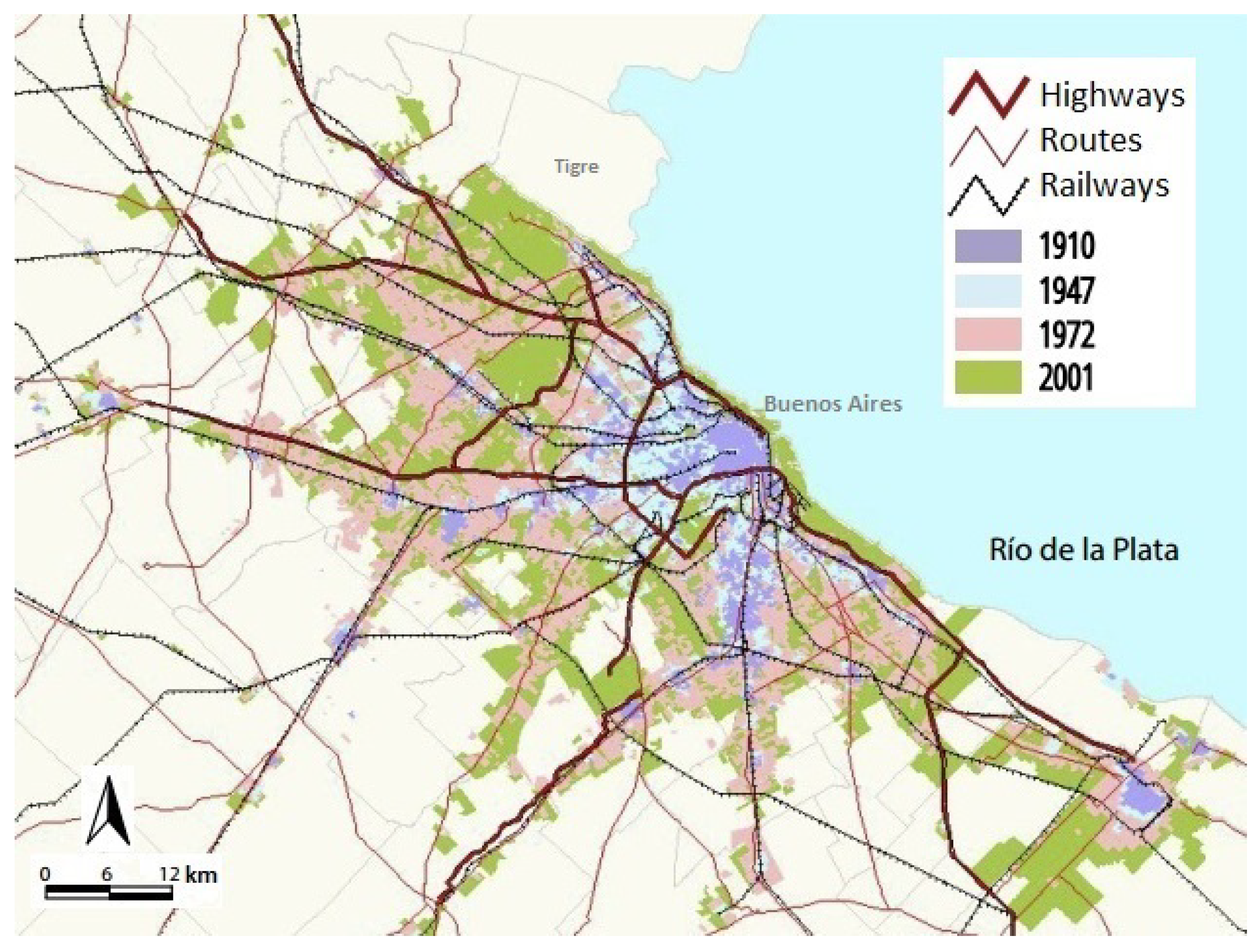
It should be noted that the urbanisation process of the AMBA has been closely linked to the development of transport infrastructures (see Figure 1). The growth of the urban area began at the time when guided transport systems were spreading. It first took place along the railway lines and the subsequent introduction of buses enabled mobility into the interstitial spaces. In fact, at the turn of the 20th century, the AMBA was at the vanguard of the most developed areas in terms of guided transport systems (its first underground railway line, a pioneer in Latin America, opened in 1913). However, it is currently lagging behind metropolises such as Mexico City and São Paulo. Since the mid-1970s, investment has been focused on the motorway network, with reduced spending on rail and underground lines, thus weakening the backbone of mass mobility [35]. While intra-urban public transport maintained some standard of quality and carries hundreds of millions of passengers per year, inter-urban transport has fallen into an almost terminal crisis [35,38], exacerbating the problems of the most vulnerable sectors of society by reducing their access to housing, employment, and consumption [35]. In parallel, the use of private vehicles became widespread in the last quarter of the 20th century, later than in other Latin American metropolises, as investment in public transport systems was not sufficient to meet the growing demand for urban mobility [34]. As a result, guided transport systems dropped from 12.3% to 8.7% of total journeys from 1970 to 2006, while individual motor vehicle use rose from 15.2% to 40.4% [35].
The AMBA currently has an extensive public transport system (276 bus lines, 8 rail lines, 6 underground lines, and the tramway in the CABA), but the infrastructure is poor (particularly the railway lines), and deployment is uneven (too many radial and not enough transversal routes) [38]. This implies that despite its wide coverage, the transport network is inadequate when it comes to dealing with the significant daily volume of traffic, particularly in the peripheral areas [26,34,38]. We should bear in mind that the transport organisation in the AMBA depends on four unrelated jurisdictions (the national government, the government of the CABA, the Buenos Aires provincial authorities, and municipal authorities), which results in poor coordination with respect to investment in infrastructure and management of transport systems.
To conclude, the AMBA has developed through expansive and unregulated patterns of urban growth, with a certain spatial continuity, but with no administrative structure. The lack of coordination in urban planning combined with a lack of vision in terms of spatial planning with respect to transport networks have resulted in a poor and unsustainable mobility model [40].

2.2. Commuting in the AMBA. The ENMODO Survey

The Household Mobility Survey, ENMODO [41] conducted in the AMBA between late 2009 and early 2010 is the main source of data used in this study. The aim of this survey was to collect information to quantitatively and qualitatively characterise the mobility patterns of the inhabitants of the AMBA on a typical working day.
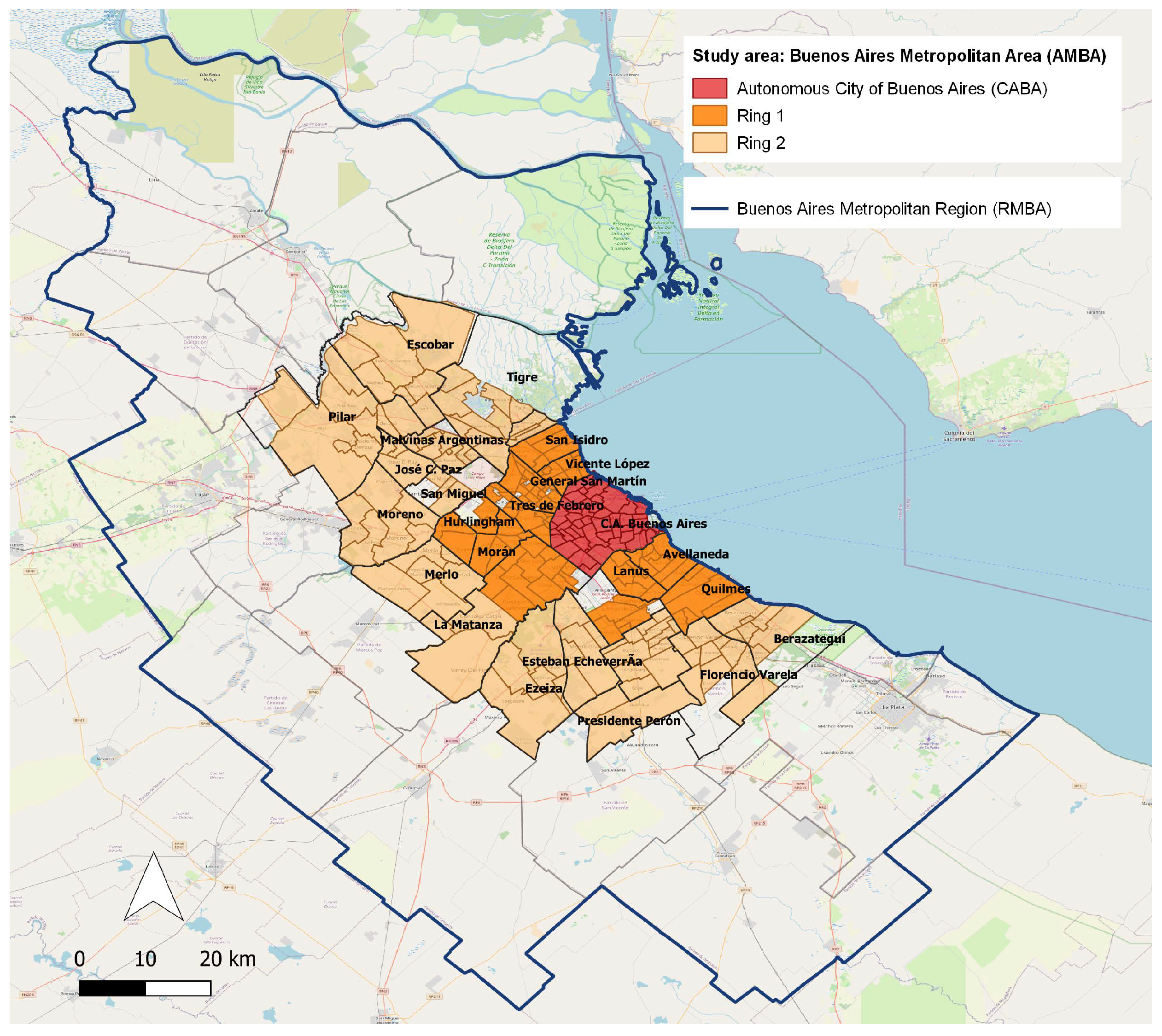
As stated above, the AMBA has a dynamic make-up, and its boundaries are moving as the “urban sprawl” around the CABA spreads, adding new municipalities to the Buenos Aires conurbation in the process. The specific study area of the ENMODO survey was limited to a group of municipalities, selected on the basis of the continuity of the urban fabric and the number of inhabitants. The defined area covers the territory comprising the CABA and 27 municipalities of the province of Buenos Aires located in the first two peripheral rings1 (see Figure 2). The sample design of the ENMODO survey corresponds to the information from the 2001 census. The distribution of the sample ensured equal geographical representation between the research population and the total population throughout the study area. A total of 22,500 households was surveyed, at a rate of one household in every 150, a ratio recommended for areas of the magnitude of the AMBA. Information was collected about every member of the household who had made trips on the day prior to the day they were surveyed. The survey questions covered both mobility aspects and socio-economic characteristics. The final number of effective surveys correspond to a total of 22,170 households and 70,321 people.
The ENMODO data show that in 2010, a total of 4.9 million daily trips were made within the CABA, 2.8 million between the CABA and the surrounding municipalities, and 9.3 million between the municipalities in the conurbation. More than half of these journeys are related to occupational mobility: 37.4% for travel to work and 25.1% for travel to school or college. Next came journeys for accompanying a member of the household to school (8.8%), shopping (7.4%), personal business (4.7%), and health (4.2%). Our study focuses specifically on single-stage journeys from home to work. These trips account for 84% of total commutes, which proves that the number of trips involving changing modes of transport is small [41]. Commuters used public transport in 45.6% of these journeys (38.4% by bus, 3.7% by underground, and 3.5% by rail), private vehicles in 35.8% (30.2% by private car and 2.9% by motorcycle), and non-motorised modes in 18.6% (13.2% on foot).
We carried out a detailed analysis of commutes exploiting the data in the ENMODO survey. The AMBA has been broken into three areas, the CABA and the first two metropolitan rings (see Figure 2) in order to get more in-depth information on commuting patterns. According to our results shown in Table 1, we observe that Ring 1 is the area that gives rise to most journeys to work (41%), while CABA is the main destination (41%). Moreover, we obtain that three quarters of the journeys have their origin and destination in the same area, which implies that, not only is the population scattered, but that there also appears to be an increase in jobs in the rings. On the other hand, Table 2 shows that the use of public transport to commute within the capital is twice that of private transport, while the modal distribution is quite balanced for journeys within the rings. By contrast, inter-zonal commutes represent only 25% of the total and mostly use private transport, with the exception of those from Ring 1 to CABA and from Ring 2 to Ring 1, which mainly use public transport. It should be noted that the extent to which each mode of transport is used is partly explained by the availability of public transport. While bus journeys are evenly distributed throughout the AMBA, 2/3 of all rail journeys take place in the northern area, and the localities in Ring 2 that are not served by rail services have difficulties accessing the CABA [42]. Finally, we can see that around 30% of the commutes within Rings 1 and 2 are made on foot and by bike. This may be partly due to the fact that most of the precarious, interstitial areas are located in these rings. These areas are far from being bicycle and pedestrian friendly, yet walking and cycling are necessary because people have to leave their own neighbourhoods to carry out any activity, including accessing public transport [36].
The ENMODO mobility survey also reveals differences in the mode of transport used by commuters from different socio-economic groups. Firstly, comparing the mobility patterns of the lower and higher income groups, we find that use of private transport increases from 19% in the former to 31% in the latter, while non-motorised modes decreases from 22% to 13%, respectively. Public transport is the most widely used mode among all income groups, but there are differences: Buses are used by 46% of low-income commuters and 39% of high-income commuters, while underground use goes from 2% (low income) to 9% (high income). We also found differences in mobility depending on the kind of jobs. Public transport is the most widely used mode among unskilled workers, while employers/entrepreneurs and professionals tend to use private transport more. The use of non-motorised trips is concentrated in the unskilled workers group. Finally, the survey data reveal clear differences in the modes of transport used by men and women. For example, men use private cars on 28% of their commutes while women only do so in 8% of cases. Women also travel more on public transport (50% of women’s journeys are made by bus as opposed to 37% of men’s trips) and on foot (16% among women and 10% among men). These findings are consistent with other studies conducted in Latin America [2,43] which have found that women, particularly those from low-income groups, often have no access to private vehicles and have to use public transport. Furthermore, women also tend to work closer to home and are thus more likely to use non-motorised modes.

3. Urban Development and Modal Split in Commuting: Methodological Framework

In this section, we develop the methodology applied to analyse the influence of urban development factors on modal split in commuting to help policymakers design integrated urban and transport policies in the AMBA.
Since the 1990s, municipal governments have had the power to regulate land use, allowing them to position themselves as promoters of local development [40]. However, when choosing the observation unit for this analysis, we opted for a higher level of disaggregation to allow us to better characterise land use factors, mainly those related to urban design that are important for all journeys, particularly non-motorised ones [6]. To achieve this goal, we have taken the administrative structure of the AMBA into account. In Argentina, municipalities are divided into smaller administrative units known as localities (localidades), while the 15 communes of the CABA are divided into neighbourhoods (barrios). In all, we worked with 241 observations, 47 neighbourhoods, and 194 localities. Please note that from this point on, we will use the term locality to refer to both the localities themselves and the neighbourhoods.
Lastly, the findings of this study correspond to the locality level, and the effect of changes in urban development on mobility observed at this level cannot necessarily be extrapolated to lower or higher levels [44].

3.1. Modal Split and Its Determinants: Theoretical Model

In this study we have classified single-stage commutes from home to work in three categories, depending on the mode of transport used: Private (car driver or passenger, motorcycle and taxi); public (rail, underground and bus); and non-motorised (cycling and walking). The modal split indicators for every locality are defined as the proportion of commutes in each category: (i) Private transport (PRIV); (ii) public transport (PUB); and (iii) cycling or walking (WALK). The quantile maps in Figure 3 show how these three variables are distributed across the localities: The darker the colour, the higher the proportion of commutes in that specific mode of transport. The patches of the same colour seen on the maps indicate that the spatial distribution of the modal split variables is not random: There is a tendency for localities with similar figures to group together (especially for private and public transport). This effect is known as spatial correlation. This result suggests that, in these cases, territory can play an important role as a source of externalities, something very commonly associated with transport infrastructures.
The land use factors considered in explaining the modal split are selected based on previous research. The earliest empirical studies point out that the characteristics with the greatest repercussions are density, diversity, and (urban) design, which Cervero and Kockelman [45] refer to as “the 3Ds”. Later, the number of factors were extended to five, known as “the 5Ds”, with the addition of access to destinations and distance to transit [5]. The theoretical model we propose is based on the 5Ds, which have been shown to work well in explaining the links between land use and mobility patterns in developed countries, particularly the US [11]. We classified the first “3Ds” as land use factors, and the other two as characteristics of public transport (see Table 3).
The specific explanatory variables selected depend largely on the data available. The first one is population density (GPD), a key factor in this kind of analysis. The second “D”, diversity, is usually factored in by using functional mix indicators such as the jobs/residents ratio as a proxy. The lack of employment data for the AMBA at a locality level available for 2010 led us to use the commuting self-containment capacity (SC) variable as an alternative [46]. This variable measures the ratio between commuters moving within the locality to go to work and total commuters in that locality. High scores may indicate localities that feature a blend of residential and work functions, while very low scores may denote localities that are mainly residential [47]. Urban design is included by means of two variables on street network characteristics: Street intersection density (SID) and street density (SD) [5,6,48]. Both variables are estimated using information from OpenStreetMaps and include thoroughfares of all types (motorways, pathways, primary, secondary, tertiary, residential, footways, etc.). The variables linked to the characteristics of public transport include distance to transit (DT) and destination accessibility (DA). They are both measured as the average number of blocks walked from home to the starting public transport stop and from the arrival public transport stop to the workplace, respectively. It should be noted that this information is only available for commuters that use public transport, which is clearly a limitation in this analysis.
2 Finally, we also include a variable that reflects the diversity of public transport supply at each locality (PTS). The available information on the public transport network shows that one locality has no public transport, 85 localities only have access to bus services, and 155 localities have conventional train or underground services in addition to the bus. Within this last group, a distinction must be drawn between more peripheral localities, which only have access to conventional train services, and 30 localities in the CABA, with underground services. Given the good reputation of the underground among its users, including those of a medium-high socio-economic level [49], we considered that it should be treated as a different category from having only conventional train services. Accordingly, the PTS variable takes the value 0 for localities with no public transport or with only bus services; 1 for the 125 localities with bus and conventional train services, and 2 for the 30 localities with underground services, regardless of whether they have access to other public transport services. Since the value of this variable is 2 only when the underground is included, we could say that the PTS variable reflects not only the diversity of public transport in a locality but also gives, to some extent, an idea of its quality.
Like many other Latin American cities, our study area is characterised by strong social inequalities (in terms of income, education, gender, etc.), an aspect that needs to be taken into account when studying mobility and transport [2,10]. Following this line of work, we would like to analyse whether these very specific socio-economic characteristics could influence the effectiveness of transport policies. To identify these socio-economic profiles, we propose to group the localities based on the similarities reflected in the information available in ENMODO on income, cars per household, percentage of women, size of the households, education level, and occupation (see Table 3). To achieve this goal, that is, to identify possible areas of socio-economic homogeneity throughout the AMBA, the cluster analysis method was chosen [50].
Cluster analysis is a statistical technique that aims to form groups of similar entities, maximising similarities between localities in the same cluster and minimising similarities between localities in different clusters. For the analysis presented here, an agglomerative hierarchical k-means clustering approach was adopted, which is a combination of the most commonly used methods, hierarchical, and k-means clustering. The procedure to determine the clusters is as follows. Firstly, we select the Manhattan metric to measure the (dis)similarity between every pair of localities in the data set. Secondly, we apply the agglomerative clustering method, which works in a “bottom-up” manner. That is, each object is initially considered as a single-element cluster. At each step of the algorithm, the two clusters that are the most similar are combined into a new bigger cluster using the Ward’s minimum-variance method [51]. This procedure is iterated until all points are members of just one single big cluster. We do not want only one cluster, so following the k-means clustering technique, it is necessary to determine where to cut the hierarchical tree into clusters. It is not easy to answer the question about how many clusters should be created. We have calculated the optimum number of clusters, 3 in our case, using the Gap statistic [52], which guarantees a cluster structure as far removed as possible from random uniform distribution.
As it may be observed in Table 4, each of the resulting clusters has its own combination of the variables used to determine them, shaping up its own socio-economic profile. The analysis of the means of the socio-economic variables for each cluster reveals that Cluster 1 comprises 71 “well off” localities with high levels of income, motorisation, education, and qualified workers, while, at the other extreme, Cluster 3 comprises 75 localities characterised by low levels of the same variables. Finally, Cluster 2 contains 95 localities with medium scores for the majority of the variables.
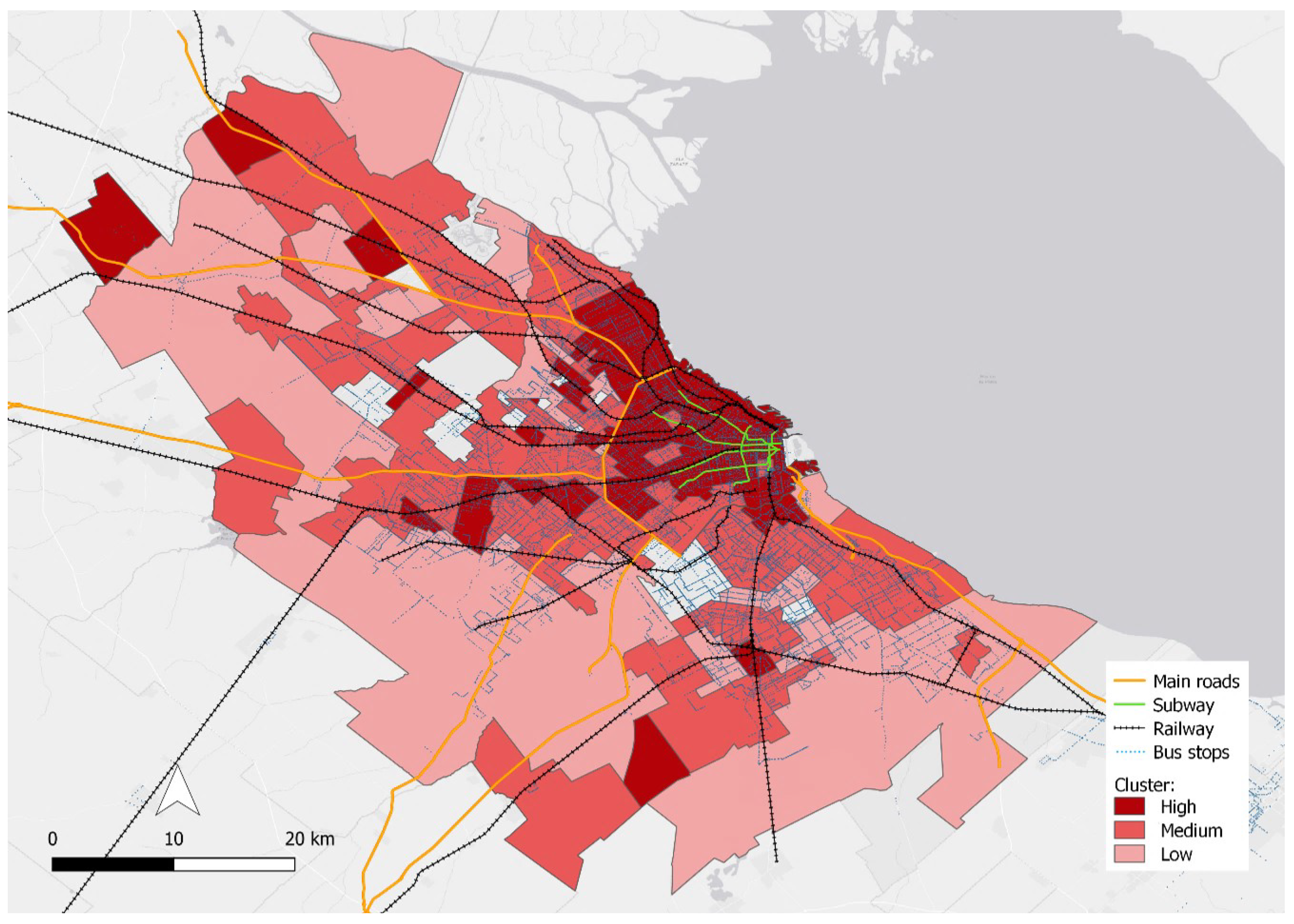
Figure 4 shows the spatial distribution of the socio-economic clusters. It can be seen that the process of metropolitanisation has led to the various socio-economic profiles being located in very specific geographical areas. The localities with a high socio-economic profile (Cluster1) are concentrated mainly in the CABA and in some peripheral areas close to the motorway network, as pointed out in Section 2. The localities with a medium socio-economic profile (Cluster2) expand like tentacles along the axes formed by motorways and public transport lines. Finally, those with a low socio-economic profile (Cluster3) are located in peripheral areas with little access to main thoroughfares, and in interstitial areas that are poorly served by public transport.
One of the hardest issues to resolve in this kind of analysis is the direction of causality, since people may not choose their place of residence randomly but based on their preferences for mobility or attitudes to transport. Therefore, the correlations observed between land use factors and modal choice may reflect the complex relationship of these factors with others, making it hard to separate the net effect of land use factors on mobility. This phenomenon, known as residential self-selection, creates estimation biases that may result in the effect of land use on modal split being either overestimated or underestimated [5,53]. This problem may come from two sources, attitudes and sociodemographic traits [54]. Several lines of research have been undertaken to address this complex issue [53]. They range from the inclusion of attitude towards transport variables [55,56] or socio-economic factors [57,58], to the use of longitudinal approaches [59,60]. The ENMODO survey provides no information on attitudes to transport that we may use. We expect that the inclusion of the socio-economic profiles of the localities in the model may help us to reduce some of this self-selection bias.

3.2. Spatial Econometric Model

The methodology used to analyse the relationship between urban development characteristics and modal split in commuting is based on regression analysis. As observed in Figure 3, the spatial distribution of the share of each mode of transport is not random rather, there are groups of adjacent localities that show similar characteristics in terms of mobility patterns, which is not unusual when working with variables observed at the same points in space. This means that the assumption of independent observations, which is basic to regression analysis, may not be met. Spatial econometric techniques make it possible to explicitly factor this spatial dependence structure into the model so that the estimates and the inference from the regression model are correct [29].
In order to include the spatial effects in a regression model, it is necessary to define the spatial dependence structure, which is of a multi-directional nature. This objective is achieved by defining non-stochastic spatial weights or contacts matrix, W = [ w i j ] , whose elements reflect the degree of interdependence between each pair of points in space, in our case between localities. The spatial lag for a variable is then constructed by simply pre-multiplying the matrix W by the said variable.
Spatial autocorrelation can be included in the regression model either by allowing the error term to be spatially autocorrelated or by including the spatially lagged dependent variable as an explanatory variable. The reason for specifying a spatially autocorrelated error may be based on the possible omission of spatially correlated random factors or on mismatches between the spatial scale of the process and the spatial scale of the observations (usually administrative units). By contrast, the motivation for including a spatially lagged variable in our model is usually for theoretical reasons such as the spillover effects of transport infrastructures or the interaction between locations [14], although it may also reflect scale problems in the data. The so-called general spatial model incorporates spatial dependence both in the error term and in the dependent variable [61] and is capable of representing very flexible patterns of spatial interrelations and/or spillovers:
y = X β + ρ W y + u w i t h u = λ W u + ε
where y is the vector ( N × 1 ) of observations of the dependent variable, X is the matrix ( N × k ) of observations of the k explanatory variables, β is the vector ( k × 1 ) of regression coefficients, and u is a vector ( N × 1 ) of error terms that follows a spatial autoregressive process. Variables W y and W u are known as spatial lags of y and u respectively, and ρ and λ are their autoregressive spatial coefficients. There is no universally accepted definition for the spatial weights matrix W = w i j . If the structure of the interdependence of the different spatial units is not known, the physical first-order contiguity criterion proposed by Moran [62] is usually used, where w i j is 1 if regions i and j are physically adjacent, and 0 otherwise. Finally, given that the homoskedasticity assumption may not be fulfilled in many applications due to the heterogeneity of the spatial units, e.g., in terms of population or area, we use the general assumption that innovations ε are independent, with zero mean and non-constant variance.
The methodological approach we adopt is to start by estimating the general spatial model (1) and if a test of the joint hypothesis of no spatial autocorrelation concludes that the coefficients, ρ and/or λ are not statistically different from zero, a reduced version of model (1) with only a spatial error or spatial lag dependent variable will be considered.
Regarding the appropriate estimation method for model (1), we have to take into account, firstly, that the ordinary least squares (OLS) estimators are not consistent because the presence of the spatial lag, W y , introduces problems of endogeneity since it is usually correlated with the disturbance u. Secondly, maximum likelihood estimation is based on the assumption that the innovation is independent and homoskedastic. Kelejian and Prucha [63] propose a two-stage estimation method (2SLS) that alternates a generalised moments (GM) estimator for λ with instrumental variable (IV) estimators for ( β , ρ ), providing consistent and asymptotically normal estimators under the assumptions of both homoskedasticity and unknown heteroskedasticity.
The inclusion of the spatial lagged variable, W y , implies that the spatial regression model (1) is non linear, which have implications in the interpretation of the impacts of the explanatory factors on y. The weights matrix, W, is usually standardised by rows, so the variable W y = j w i j y j is a weighted average of the values of y in the neighbouring localities. The reduced form of model (1) is given by:
y = ( I ρ W ) 1 X β + ( I ρ W ) 1 u = ( X + ρ W X + ρ 2 W 2 X + ρ 3 W 3 X + ) β + ( I ρ W ) 1 u .
Equation (2) shows that the dependent variable y for a given locality is a function not only of its own characteristics (X) but also of those of the neighbouring localities ( ρ W X , ρ 2 W 2 X , …), albeit with a factor that decreases with distance. As a consequence, the total effect of a change in a variable X i in a locality is:
E ( y | Δ X i ) = ( I ρ W ) 1 Δ X i β = Δ X i I β + ( ρ W + ρ 2 W 2 + ) Δ X i β .
We observe that the total impact is greater than Δ X i β , i.e, the presence of a spatially lagged dependent variable generates a spatial multiplier effect. Moreover, this effect depends on all the X and their spatial lags, generating feedback effects. Thus, a change in X i in a given locality j will affect the dependent variable for locality j (direct effect = Δ X i I β ) and the dependent variables for all the other localities (indirect effect = ( ρ W + ρ 2 W 2 + ) Δ X i β ) [61].

4. Empirical Analysis: Results and Implications

The results obtained when estimating the general spatial model (1) for the three modes of transport considered (PRIV, PUB, and WALK) show that the spatial error term is never significant, and the spatial lag term is significant only for private and public transport. This is not an unexpected result, since walking or cycling journeys only cover a short distance and are supposed to depend on the characteristics of the locality itself, but not on those of the neighbouring localities. Therefore, we estimate the appropriated reduced models: The spatial lag model for private and public transport and the non-spatial linear regression model for walking/cycling:
P R I V i = X i β + ρ W P R I V i + u i i = 1 , 2 , , 241
P U B i = X i β + ρ W P U B i + u i i = 1 , 2 , , 241
W A L K i = X i β + u i i = 1 , 2 , , 241
where X is a vector including land use factors (gross population density, commuting self-containment, street intersections density, and street density), characteristics of public transport (distance to transit, destination accessibility, and public transport supply) and high and medium socio-economic profiles via the dummy variables Cluster1 and Cluster2 which take values of 1 if the locality belongs to Cluster1 or Cluster2, respectively, and 0 otherwise.
Given the presence of the spatial lag, models (4) and (5) are estimated using spatial two-stage least squares (S2SLS) and model (6) by OLS, always under the general assumption that the error term u may present unknown heteroskedasticity and/or spatial autocorrelation. Accordingly, Table 5 and Table 6 show the estimations for the coefficients and the levels of significance for three standard errors calculated under different assumptions: Homoscedasticity and no autocorrelation (Classical), heteroskedasticity (White correction), and spatial heteroskedasticity and autocorrelation (SHAC) [64]. We believe that it is preferable to go for robust results if they lead to different levels of significance. As can be observed, the conclusions concerning the significance of the variables barely change, though the results provided by the SHAC standard errors are slightly more conservative.

4.1. Main Findings and Discussion

Table 5 and Table 6 show that land use factors influence the patterns of modal split in commuting in the AMBA, although there are important differences depending on the mode of transport. Private transport use depends on all land use variables except commuting self-containment capacity. Thus, the share of private transport is larger in those localities with lower population densities, lower street intersection density, and higher street density. By contrast, public transport use is positively linked to population density and street intersection density and negatively linked to self-containment capacity. Finally, non-motorised trips depend positively on commuting self-containment and street intersection density and is negatively linked to the density of roads.
In general, the results obtained are similar to those of previous studies carried out in the US and Europe in the sense that we also find evidence of the effect of land use factors on modal split [4,5,7]. However, our findings about the relative importance of these factors present some differences. While our results confirm that street design variables are highly relevant in explaining modal choice as happens in the US, on the other hand, they show that density still plays an important role in determining the share of private and public transport in the AMBA, which is more in line with the results obtained by Guerra et al. [21] for Mexico than with the conclusions of Cervero et al. and Naes [5,7].
The spatial lag is a statistically significant variable for private and public transport which means that there are spatial effects that are not captured by factors included in the model. According to Equation (2), this result implies that the use of both private and public transport depends not only on the characteristics of a given locality but also on those of its neighbours. If the urban characteristics of a given locality (low population density, low intersection density, and high street density) favour private vehicle use, the fact that adjacent localities have these same characteristics will result in an increase in vehicle use throughout the area. Commuters in a given locality may also benefit from the fact that the urban characteristics of adjacent localities (high population density or high street intersection density) meet the minimum requirements for having efficient public transport. Conversely, the presence of public transport in a given locality may benefit the adjacent ones. This result suggests the existence of spillover effects associated with transport network characteristics, which have effects that extend beyond the limits of one locality and encourage use of public/private transport in adjacent areas, although it could also in part depend on the data scale. We should bear in mind that mobility does not recognise borders and goes beyond administrative limits. Commuters usually cross several localities and our result suggests that the mode of transport used depends partly on the characteristics of all of them.
If we look in detail at the total impact of land use factors, transport characteristics, and socio-economic profiles on the modal split in commuting (see Table 7), we can see that population density has a significant impact only in relation to both private and public motorised transport. The magnitude of the total impact is similar but with opposite signs, i.e., low densities are conducive to private transport use and high densities to public transport use. These results coincide with previous research linking higher density areas to better transit service (increased demand makes it more cost effective) and a reduction in private transport due to worse driving conditions (reduction in traffic speed and parking supply, increase in traffic congestion) [4,6,21]. However, our results differ from previous research not only in the US but also in Latin America [22] that claimed that density brings destinations closer together and encourages non-motorised travel. In the AMBA, the increase in density is not sufficient to encourage travel on foot or by bicycle, probably because it does not necessarily mean that the workplace is close to the place of residence.
A high self-containment capacity, as a result of a good functional mix between work and residence enables a locality to retain its workforce, thus meaning that the distance between home and work is likely to be shorter. Previous studies in the US claimed that the direct consequence of this is a greater use of non-motorised mode [5], while some research in Latin America shows that functional diversity does not affect walking/cycling trips [22,24]. Moreover, the effect of this variable on motorised transport is not so clear either. In some situations, suburban dispersion of employment can reduce the average commuting distance, although it tends to increase total per-capita vehicle travel [6]. Other authors find that functional mix have a small and negative effect of vehicle travel but a positive one in public transport [4,5]. In the AMBA, this factor does not affect private transport trips while it is highly relevant to non-motorised and public transport journeys. The results show that a higher diversity in a locality encourages people to walk or cycle to go to work but reduces the use of public transport. The latter result could imply that workers use public transport for longer journeys outside their locality but commute on foot or by bike when they work and live in the same locality.
The urban design variables are, in general, highly significant to explain modal split. Street intersection density as a key factor for connectivity is one of the most relevant variables for modal split, affecting both motorised and non-motorised modes [5,20,48]. The average number of intersections in the AMBA is 167 and UN-Habitat considers that a score of 100 intersections means that a city is more suitable for non-motorised trips [65]. The observed positive impact on public transport and walking/cycling can be explained by the fact that more intersections means more crossing points, thus shortening distances. By contrast, the negative impact of this variable on private transport may be due to the fact that too many intersections can lead to congestion, which cannot be avoided by using a system of exclusive lanes such as the one available for rapid bus transit [6]. Finally, previous research does not provide a conclusive result on the relationship between street density and the mode of transport used. The reason is that different street systems with the same network density may have different effects [66]. Street density does not reflect whether streets are station-oriented, pedestrian friendly streets, or highways. In our study, the SD variable includes all types of roads, from footpaths, which are specifically for non-motorised mobility, to motorways, which require the use of vehicles. This may explain why street density in the AMBA has a substantially positive impact on private transport, in line with previous studies [10,16]. The negative impact of street density on non-motorised trips may be explained by the fact that walking and cycling conditions are also affected by other urban design characteristics, such as the quantity and quality of pavements, pedestrian crossings and paths, and the safety and attractiveness of routes [67,68]. Therefore, a higher street density does not necessarily mean more journeys on foot or by bike.
As far as the variables related to public transport are concerned, distance to transit and destination accessibility are considered relevant factors in public transport. In fact, previous studies show that they are the most important factors for motorised transport [5] and that there is a significant decrease in the use of public transport as walking distance to bus stops or stations increases [10,69]. By contrast, our results for these two variables are not significant. This conclusion may be partly due to the fact that many travellers have no alternative but to use public transport even if it is not very accessible, since they do not have a car and cannot reach their workplace on foot or by bicycle, but another part may come from the design of these variables in the AMBA. As mentioned above, given the available information, these variables only measure the distance travelled by public transport users both to public transport stops and to their destination. In other words, they only include distances below a certain threshold that ensure a degree of accessibility to public transport. They do not include longer distances that make public transport not so accessible, and that may favour non-motorised travel if the home-work distance can be covered walking or cycling, or car travel if that is not the case.
As expected the public transport supply variable has a substantial impact on the use of motorised transport in the AMBA: The broader the range of public transport, the more public transport and the less private vehicles are used. This is in line with the results of other studies which indicate that car travel tends to decline when there is a strong, competitive transit system [6]. Concerning non-motorised trips, even though the sign of the coefficient is negative as expected, the variable is not significant. Therefore, we may conclude that in the AMBA, a wider variety of public transport does not significantly affect walking or cycling journeys, while, for instance, Guerra et al. [21] obtains that in Mexico commuters are more likely to use this mode in areas with a broader public transport supply. Our result may be due to the fact that commuters tend to use public transport only when the distance is too great to travel by bicycle or on foot, and yet prefer to walk or cycle if the distances are short enough, whether or not public transport is available. According to ENMODO data, the average distance travelled by public transport is 7.1 km, while walking or cycling trips cover around 1.8 km. It should be also taken into account the negative reputation of certain public transport, mainly the conventional rail service (delays, cancellations, overcrowding, etc.) and the low purchasing power of the population.
The results obtained show that the socio-economic profile of a locality has a high impact on modal split. As expected, the proportion of public transport and non-motorised travel is lower the better the socio-economic situation of a locality. Note that the use of public transport in the high-level cluster is 11 points below its use in the least privileged localities. By contrast, localities with the lowest socio-economic profiles use private transport in a much lower proportion compared to other profiles: 17 points below the localities belonging to the “high-level” cluster and 10 points below the localities with a “medium” profile [10]. Our conclusions confirm the results obtained in previous research on this topic that show that socio-economic factors not only are highly relevant to explain modal split but sometimes they are even more important than urban development factors [21,22,24].
Finally, as explained in Section 3.2, the presence of the spatial lag generates feedback effects in the models for private and public transport. Thus, the total impact of a change in a variable X i for a given locality can be divided into direct effects, which remain in the locality, and indirect effects or spillovers that affect other localities (see Equation (3)). The analysis of the results shown in Table 7 gives an idea of the strength of these feedback effects. Firstly, it may observed that the direct impact of each variable is very similar to the coefficient estimate. This means that the locality where the change occurs does not receive much feedback from other localities. Secondly, the indirect impacts of each factor are not very significant with the exception of the results obtained for private transport. This conclusion may be due to the fact that spillover effects come from the inclusion of a spatial lag, which is a combination of all the explanatory variables, and it does not seem easy to isolate and assign them to a specific factor. In the case of private transport, indirect impacts of population density, street intersection density, public transport supply, and socio-economic profiles are significant. This means that a locality surrounded by others with low levels of population density, connectivity, and public transport supply will tend to use private vehicles more. Private transport becomes the main option when population density is not sufficient to provide efficient public transport in the area.

4.2. Effectiveness of Public Transport Policies

As pointed out above, the supply of public transport affects motorised mobility, increasing the use of public transport and reducing the use of private vehicles. This suggests that policies aimed at improving the public transport system would help to redirect mobility towards a more sustainable model. However, the results also show that, all things being equal, the use of the private transport is significantly higher in localities with high and medium socio-economic profiles than in those with a lower profile, while the use of the public transport is significantly lower. These differences are so large that they make us wonder whether all localities would respond similarly to policies aimed at promoting public transport, regardless of their socio-economic profiles. As a first approach to test this hypothesis, we include a set of interaction terms in models (4) and (5) combining socio-economic profiles (clusters) and public transport variables in order to allow the impact of these variables to differ from one cluster to another. Note that the low socio-economic profile, Cluster3, is the reference group chosen.
The results in Table 8 might help to refine our earlier conclusions. Firstly, we found that the impact of changes in public transport supply have no significant effect in localities with a low socio-economic profile (Cluster3) for both private and public transport. This result can be partly explained by the fact that less than 26% of households own a vehicle, so private transport use is low and limited, probably intended for long journeys not covered by public transport (secondary roads, sparsely populated areas, etc.). Even if transit supply were increased in these localities, it is unlikely that public transport would cover these routes and the use of private vehicles would still be necessary. Secondly, the difference in the impact of public transport supply between localities in Cluster3 and the well-off localities in Cluster1 is not statistically significant. This result suggests that in the latter, where 46% of households own a vehicle, a broader public transport supply is unlikely to lead to any significant change in mobility patterns. Note that these are the only localities that have underground services, which are used even by families that have their own vehicles [41]. However, getting these people to switch from cars to buses or trains seems to be no easy task, given the negative reputation of public transport, particularly trains [49]. To achieve this goal, it would be necessary to change their perception of public transport by improving the safety and security, comfort, and the objective aspects of journey time and frequency of the modes of transport concerned [70]. Finally, in those localities with a medium socio-economic profile (Cluster2), the effect of improvements in public transport supply is significant and leads to increases in public transport use and decreases in private car use. Around 36% of the households in these localities have access to private vehicles, but it seems that some would be willing to switch to public transport for commuting if the offer were improved.
The previous result indicating that destination accessibility (DA) do not influence average mobility patterns is slightly modified by the results shown in Table 8. Once again, greater distances from the public transport arrival stop to the workplace result in less use of public transport only in localities with a medium socio-economic profile. In short, it could be concluded that measures to promote the diversity of the public transport supply and to improve its accessibility could increase demand, particularly in localities with a medium socio-economic profile. It seems that, on average, the commuters in these localities have more access to private transport than Cluster3 on the one hand and less resistance to switching to public transport than Cluster1 on the other.
5. Conclusions

This paper studied the relationship between urban development and mobility patterns in the Buenos Aires Metropolitan Area by performing a spatial econometric analysis of the links between land use factors, public transport characteristics, and socio-economic profiles on the use of specific modes of transport in commuting. In general, our results are similar to those obtained by previous research carried out in the US and Europe [5,6,7], suggesting that land use factors and public transport characteristics are also significant in explaining mobility patterns in Latin American countries. This implies that urban and transport policies may be useful in managing the demand for mobility and encouraging the use of sustainable modes of transport.
In particular, it appears that population density influences motorised transport in the AMBA but is not sufficient to encourage non-motorised travel, which requires the workplace to be close to home. The latter concept is best captured by the self-containment capacity variable, the results of which show that it affects both public transport and non-motorised travel. As far as urban design variables are concerned, the street intersection density appears to be a key factor in influencing both motorised and non-motorised trips. However, the results obtained for the variable street density, which show a positive impact on private transport and a negative one on non-motorised journeys, are not easy to interpret. It should be noted that the results for this variable vary greatly [71,72], which may be due to different street systems with the same network density having different effects [66]. It is possible that the street network characteristics in our case study are more favourable to the use of the car than to non-motorised journeys. We should also bear in mind that walking and cycling depend not only on street density but also on other factors related to the safety and security, connectivity, and attractiveness of the route. In this regard, recent public policies promoting cycling in part of the CABA, such as the construction of cycle lanes and the establishment of public bike-lending systems, are positive. However, the point is that, in order to be more effective, they should also extend to the most precarious areas, where this type of journey has the greatest weight. To sum up, in terms of land use policies, densification, functional mix, and an adequate urban design may help to reduce the use of private vehicles, promote public transport, and facilitate walking and cycling.
We also found evidence that motorised mobility patterns in a given locality depend on its characteristics and on those of its neighbours, i.e., mobility does not recognise borders and goes beyond administrative limits. A total 79% of commutes in the AMBA cross several localities and our result suggests that the mode of transport used depends partly on the characteristics of all of them. Consequently, policymakers should pay attention to spatial effects, since urban policies that change land use characteristics in a locality may affect modal split not only in that locality but also in nearby localities as well. They also need to coordinate and articulate those administrative structures that influence urban policies and promote intermunicipal cooperation organisations, given that those existing in the AMBA are currently scarce [40]. Furthermore, the presence of spatial dependence may also reflect the existence of transport infrastructure spillover effects, which again implies the need for the transport planning decision-making process to be coordinated at a supra-locality level. Considering the AMBA as a whole may facilitate the provision of a public transport network that covers the entire metropolitan area. This would improve access particularly to, currently, the most isolated areas, a goal that cannot be achieved by each locality separately. In addition, policymakers need to bear in mind that the problems raised by mobility vary from place to place, which requires the design of area-specific measures within an integrated transport plan. To this end, it is necessary to have institutions that are capable of overcoming the current fragmentation of transport management responsibilities in the AMBA and the existing deficiencies in some peripheral localities. In this context, some authors suggest providing the Metropolitan Transport Authority with more resources to coordinate investments throughout the metropolitan area [32].
Our results show that changes in the public transport supply affect motorised mobility, by promoting public transport use and reducing the use of private vehicles. In this respect, it is important to ensure that the public transport service is efficient and safe, in order to discourage the use of private cars. In addition, we found large differences in mobility patterns between localities with different socio-economic profiles, which could affect the effectiveness of certain transport policies. This is an important aspect to take into account, especially in countries characterised by high rates of poverty and inequality. In particular, we show that an increase in the diversity of public transport supply could promote its use, but mainly in localities with a medium socio-economic profile. This result suggests that some policies to promote/discourage the use of a certain mode of transport may be more effective if they target specific socio-economic groups. However, these conclusions should be viewed with caution, since the methodology used, based on the addition of interaction terms in the models, does not capture all the aspects of the problem analysed.
To conclude, our results reaffirm the importance of the spatial and territorial dimension in the public policy formulation process, specifically, in our case, the need to integrate urban planning instruments with those of mobility and transport.
However, some limitations of the study must be taken into account when analysing the results. This study does not take multi-stage journeys that often involve combinations of different modes of transport into account. Although this type of journey is not a common form of commuting in the AMBA, it usually involves public transport so the results for these type of journeys could be affected. With respect to the specification of econometric models, it should be noted that the functional form used is linear. Given that the dependent variables are proportions, this functional form may lead to some problems, e.g., negative forecasts. However, the focus of our analysis is on trying to determine whether the urban development factors influence modal split in commuting and to measure the strength of this relationship. In this sense, we believe that the selection of the linear approach, although a limitation, could be good enough to attain our goal. Moreover, we were unable to obtain conclusive results on the influence of variables related to the accessibility to and from public transport and street density, due to the limitations presented by the indicators chosen for them. Previous research on the key factors that influence the relationship between walking and transit could help derive indicators to measure the distance people walk to and from public transport [73]. For example, the effect of street density is different depending on the type of urban fabric formed by these streets, either traditional grid street patterns or suburban neighbourhood design.
Nevertheless, these limitations open new avenues for future research. The line of research on urban development and modal split (mainly public transport) could be completed by including multi-stage journeys. The street density indicator could be improved by constructing a composite indicator that synthesises the different aspects of this variable in a single measure, in line with the research done on walkability indices [74] or using two different variables for the road street density and the pedestrian/foortpath density. The assessment of the efficiency of public transport policies could be more accurate if done by applying other methods, such as scenario analysis.

Author Contributions

For this paper, L.M. and P.G. did the conceptualization and proposed the methodology; L.M. provided the data; P.G. carried out the formal analysis; L.M. and P.G. validated the results and wrote the paper. All authors have read and agreed to the published version of the manuscript.

Funding

This work was supported by the UPV/EHU Econometrics Research Group (Basque Government grant IT1359-19) and EKOPOL Research Group (Basque Government grant IT1365-19).

Institutional Review Board Statement

Not applicable.

Informed Consent Statement

Not applicable.

Data Availability Statement

The data presented in this study are openly available at the URL www.argentina.gob.ar/transporte/dgppse/publicaciones/encuestas.

Acknowledgments

We appreciate the members of the Centro de Investigaciones y Estudios Ambientales (CINEA) de la Universidad del Centro de la Provincia de Buenos Aires (UNICEN) for their invaluable help with the interpretation and geographical representation of the data.

Conflicts of Interest

The authors declare no conflict of interest.

References

  1. United Nations. 2018 Revision of World Urbanization Prospects; Department of Economic and Social Affaires: New York, NY, USA, 2018. [Google Scholar]
  2. Jirón, P. Sustainable Urban Mobility in Latin America and the Caribbean. Global Report on Human Settlements; Technical Report; UN-Habitat: Nairobi, Kenya, 2013. [Google Scholar]
  3. Gakenheimer, R. Transportation and Land Use in the Developing World: Planning in a Context of Controversy; International Congress on Human Development: Madrid, Spain, 2006. [Google Scholar]
  4. Aston, L.; Currie, G.; Kamruzzaman, M.; Delbosc, A.; Teller, D. Study design impacts on built environment and transit use research. J. Transp. Geogr. 2020, 82. [Google Scholar] [CrossRef]
  5. Ewing, R.; Cervero, R. Travel and the Built Environment. J. Am. Plann. Assoc. 2010, 76, 265–294. [Google Scholar] [CrossRef]
  6. Litman, T.; Steele, R. Land Use Impacts on Transport. How Land Use Factors Affect Travel Behavior. Victoria Transport Policy Institute. 2020. Available online: https://www.vtpi.org/tdm/tdm20.htm (accessed on 13 December 2020).
  7. Naess, P. Urban form and travel behavior: Experience from a Nordic context. J. Transp. Land Use 2012, 5. [Google Scholar] [CrossRef]
  8. Stevens, M.R. Does compact development make people drive less? J. Am. Plann. Assoc. 2017, 83, 7–18. [Google Scholar] [CrossRef]
  9. Zhang, M. The role of land use in travel mode choice: Evidence from Boston and Hong Kong. J. Am. Plann. Assoc. 2004, 70, 344–360. [Google Scholar] [CrossRef]
  10. Zhao, P. The impact of the built environment on individual Workers’ commuting behavior in Beijing. Int. J. Sustain. Transp. 2013, 7, 389–415. [Google Scholar] [CrossRef]
  11. Cervero, R. Linking urban transport and land use in developing countries. J. Transp. Land Use 2013, 6, 7–24. [Google Scholar] [CrossRef] [Green Version]
  12. Corporación Andina de Fomento.Desarrollo urbano y movilidad en América Latina, Caracas. 2011. Available online: http://scioteca.caf.com/handle/123456789/419 (accessed on 21 January 2019).
  13. Cao, X. Land use and transportation in China. Transp. Res. D Transp. Environ. 2017, 52, 423–427. [Google Scholar] [CrossRef]
  14. Yu, N.; de Jong, M.; Storm, S.; Mi, J. Spatial spillover effects of transport infrastructure: Evidence from Chinese regions. J. Transp. Geogr. 2013, 28, 56–66. [Google Scholar] [CrossRef]
  15. Jiang, Y.; Gu, P.; Chen, Y.; He, D.; Mao, Q. Influence of land use and street characteristics on car ownership and use: Evidence from Jinan, China. Transp. Res. D Transp. Environ. 2017, 52, 518–534. [Google Scholar] [CrossRef]
  16. Sun, B.; Ermagun, A.; Dan, B. Built environmental impacts on commuting mode choice and distance: Evidence from Shanghai. Transport. Res. Part D Transp. Environ. 2017, 52, 441–453. [Google Scholar] [CrossRef]
  17. Wang, X.; Shao, C.; Yin, C.; Zhuge, C. Exploring the Influence of Built Environment on Car Ownership and Use with a Spatial Multilevel Model: A Case Study of Changchun, China. Int. J. Environ. Res. Public Health 2018, 15, 1868. [Google Scholar] [CrossRef] [PubMed] [Green Version]
  18. Mahmud, M.; Rabbani, A. Travel Mode Choice Preferences of Urban Commuters in Dhaka; A Pilot Study, Bangladesh Country Growth Program International Growth Centre (IGC); London School of Economics: London, UK, 2012. [Google Scholar]
  19. Masoumi, H.E. A discrete choice analysis of transport mode choice causality and perceived barriers of sustainable mobility in the MENA region. Transp. Policy 2019, 79, 37–53. [Google Scholar] [CrossRef]
  20. Zegras, C. The Built Environment and Motor Vehicle Ownership and Use: Evidence from Santiago de Chile. Urban Stud. 2010, 47, 1793–1817. [Google Scholar] [CrossRef]
  21. Guerra, E.; Caudillo, C.; Monkkonen, P.; Montejano, J. Urban form, transit supply, and travel behaviour in Latin America: Evidence from Mexico’s 100 largest urban areas. Transp. Policy 2018, 69, 98–105. [Google Scholar] [CrossRef]
  22. Cervero, R.; Sarmiento, O.L.; Jacoby, E.; Gomez, L.F.; Neiman, A. Influences of Built Environments on Walking and Cycling: Lessons from Bogotá. Int. J. Sustain. Transp. 2009, 3, 203–226. [Google Scholar] [CrossRef]
  23. Rodríguez, D.A.; Brisson, E.M.; Estupiñán, N. The relationship between segment-level built environment attributes and pedestrian activity around Bogota’s BRT stations. Transp. Res. D Transp. Environ. 2009, 14, 470–478. [Google Scholar] [CrossRef]
  24. Larrañaga, A.M.; Cybis, H.B.B. The relationship between built environment and walking for different trip purposes in Porto alegre, Brazil. Int. J. Sustain. Dev. Plann. 2014, 9, 568–580. [Google Scholar] [CrossRef] [Green Version]
  25. Kandt, J. Heterogeneous links between urban form and mobility: A comparison of São Paulo, Istanbul and Mumbai. J. Transp. Land Use 2018, 11, 721–745. [Google Scholar] [CrossRef]
  26. Anapolsky, S. Los flujos de movilidad territorial. Un análisis de la población y la movilidad en el área metropolitana de Buenos Aires. Café las Ciudad. Rev. Digit. 2013, Año 12. [Google Scholar]
  27. Jakovcevic, A.; Steg, L. Sustainable transportation in Argentina: Values, beliefs, norms and car use reduction. Transp. Res. Part F Traffic. Psychol. Behav. 2013, 20, 70–79. [Google Scholar] [CrossRef]
  28. Hong, J.; Shen, Q.; Zhang, L. How do built-environment factors affect travel behaviour? Transportation 2014, 41, 419–440. [Google Scholar] [CrossRef]
  29. Anselin, L. Spatial Econometrics: Methods and Models; Kluwer Academic: Dordrecht, The Netherlands, 1988. [Google Scholar]
  30. Anselin, L. Spatial externalities, Spatial multipliers, and Spatial Econometrics. Int. Reg. Sci. Rev. 2003, 26, 147–152. [Google Scholar] [CrossRef]
  31. Instituto Nacional de Estadística y Censos de la República Argentina. Censo Nacional de Población, Hogares y Viviendas; INDEC: Buenos Aires, Argentina, 2010. [Google Scholar]
  32. Muzzini, E.; Eraso Puig, B.; Anapolsky, S.; Lonnberg, T.; Mora, V.C. Boosting the Potential of Argentine Cities: Framework for Public Policy Action: Impulsando el Potencial de las Ciudades Argentinas: Marco Para la Acción de las Políticas Públicas (Spanish); World Bank Group: Washington, DC, USA, 2016. [Google Scholar]
  33. Torres, H.A. Cambios socioterritoriales en Buenos Aires durante la década de 1990. 2001. Available online: http://www.redalyc.org/articulo.oa?id=19608003 (accessed on 22 May 2020).
  34. Goytia, C.; Cristini, M. Diagnóstico sobre Ciudades y Desarrollo Urbano; Report Coordinated by the Universidad Torcuato Di Tella and Jefatura Gabinete de la Nación: Buenos Aires, Argentina, 2017. [Google Scholar]
  35. Abba, A.P. Uso de suelo y transporte en la Buenos Aires Metropolitana. Observatorio Urbano Local Buenos Aires Metropolitana (OUL-BAM). 2011. Available online: https://www.vocesenelfenix.com/content/uso-de-suelo-y-transporte-en-la-buenos-aires-metropolitana (accessed on 12 October 2018).
  36. Gutiérrez, A.; Apaolaza, R.; Blanco, J.; Miglierina, D.; Redondo, D. Movilidad y territorio. Propuestas de ordenamiento territorial a escala barrial a partir de estudios de caso en la Región Metropolitana de Buenos Aires. In Transporte Urbano e Interurbano en la Argentina. Aportes Desde la Investigación; Müller (comp); PIUTBAT, Universidad de Buenos Aires: Buenos Aires, Argentina, 2017; pp. 97–109. [Google Scholar]
  37. United Nations. 2014 Revision of World Urbanization Prospects; Department of Economic and Social Affaires: New York, NY, USA, 2014. [Google Scholar]
  38. Rascovan, A. Organización y gestión del transporte público en el AMBA. Un recorrido histórico y perspectivas a futuro. In Transporte Urbano e Interurbano en la Argentina. Aportes Desde la Investigación; A.E.G. Müller (comp.); Universidad de Buenos Aires: Buenos Aires, Argentina, 2017; pp. 41–54. [Google Scholar]
  39. Reboratti, L. Crecimiento de la mancha urbana. Nueva densificación intersticial, consolidación de autopistas. Observatorio del Conubarno Bonaerense. 2011. Available online at BAM.21 Ambateca. Available online: http://bam21.org.ar/comunidad/mod/data/view.php?d=4&rid=253 (accessed on 25 January 2021).
  40. UN-Habitat. Política Nacional Urbana. Ministerio del INTERIOR, Obras Públicas y Vivienda; Presidencia de la Nación: Buenos Aires, Argentina, 2018. [Google Scholar]
  41. Encuesta de Movilidad Domiciliaria/ENMODO. Movilidad del Area Metropolitana de Buenos Aires; Secretaría de Transporte de la Nación: Buenos Aires, Argentina, 2010. [Google Scholar]
  42. Lordi, H. Movilidad urbana sostenible en el Area Metropolitana de Buenos Aires. Caso de éxito: Sistema de Bus Rápido (BRT-LA MATANZA). Foro de Discusión Movilidad Sustentable, UnLaM, San Junto, Buenos Aires. 2014. Available online: https://docplayer.es/2487334-Movilidad-urbana-sostenible-en-el-area-metropolitana-de-buenos-aires-caso-de-exito-sistema-de-bus-rapido-brt-la-matanza-haydee-a.html (accessed on 22 October 2018).
  43. Yañez-Pagans, P.; Martinez, D.; Mitnik, O.; Scholl, L.; Vazquez, A. Urban Transport Systems in Latin America and the Caribbean: Challenges and Lessons Learned. Development through the Private Sector Series. TN No.8, IDB-Invest.IIC. 2018. Available online: https://publications.iadb.org/publications/english/document/Urban-Transport-Systems-in-Latin-America-and-the-Caribbean-Challenges-and-Lessons-Learned.pdf (accessed on 20 March 2019).
  44. Openshaw, S.; Taylor, P.J. A Million or so Correlation Coefficients: Three Experiments on the Modifiable Areal Unit Problem. In Statistical Applications in the Spatial Sciences; Wrigley, N., Ed.; Pion: London, UK, 1979; pp. 127–144. [Google Scholar]
  45. Cervero, R.; Kockelman, K. Travel demand and the 3Ds: Density, diversity and design. Transp. Res. D Transp. Environ. 1997, 2, 199–219. [Google Scholar] [CrossRef]
  46. Camagni, R.; Gibelli, M.C.; Rigamonti, P. Urban mobility and urban form: The social and environmental costs of different patterns of urban expansion. Ecol. Econ. 2002, 40, 199–216. [Google Scholar] [CrossRef]
  47. Marmolejo, C.; Tornés, M. The Influence of Urban Structure on Commuting: An Analysis for the Main Metropolitan Systems in Spain. Procedia Eng. 2017, 148, 52–68. [Google Scholar] [CrossRef]
  48. Handy, S.; van Wee, B.; Kroesen, M. Promoting Cycling for Transport: Research Needs and Challenges. Transp. Rev. 2014, 34, 4–24. [Google Scholar] [CrossRef]
  49. Hernández, C.; Rebón, J. La calidad como reclamo. Los usuarios del sistema ferroviario de pasajeros del Área Metropolitana de Buenos Aires. In Transporte urbano e interurbano en la Argentina. Aportes desde la investigación; A.E.G. Müller (comp.); Universidad de Buenos Aires: Buenos Aires, Argentina, 2017; pp. 69–81. [Google Scholar]
  50. Kaufman, L.; Rousseeuw, P.J. Finding Groups in Data: An Introduction to Cluster Analysis; Wiley: Hoboken, NJ, USA, 2009. [Google Scholar]
  51. Ward J., H. Hierarchical grouping to optimize an objective function. J. Am. Stat. Assoc. 1963, 58, 236–244. [Google Scholar] [CrossRef]
  52. Tibshirani, R.; Guenther, W.; Hastie, T. Estimating the number of clusters in a data set via the gap statistic. J. R. Statist. Soc. B 2001, 63, 411–423. [Google Scholar] [CrossRef]
  53. Cao, X.; Chapman, D. How will Smart Growth land use policies affect travel? A theoretical discussion on the importance of residential sorting. Environ. Plan B Urban. Anal. City Sci. 2015, 43, 58–73. [Google Scholar] [CrossRef]
  54. Mokhtarian, P.; Cao, X. Examining the impacts of residential self-selection on travel behavior: A focus on methodologies. Transp. Res. Part B 2008, 42, 204–228. [Google Scholar] [CrossRef] [Green Version]
  55. Kitamura, R.; Mokhtarian, P.L.; Laidet, L. A micro-analysis of land use and travel in five neighborhoods in the San Francisco Bay Area. Transportation 1997, 24, 125–158. [Google Scholar] [CrossRef]
  56. Schwanen, T.; Mokhtarian, P. The Role of Attitudes toward Travel and Land Use in Residential Location Behavior: Some Empirical Evidence from the San Francisco Bay Area. Hous. Policy Debate 2007, 18, 171–207. [Google Scholar] [CrossRef]
  57. Frank, L.; Chapman, J.; Bradley, M.; Lawton, K. Travel Behavoir, Emissions and Land Use Correlation Analysis in the Central Puget Sound. Whasington State Department of Transportation; US Department of Transportation and the Federal Highway Administration: Washington, DC, USA, 2005. [Google Scholar]
  58. Brownstone, D.; Golob, T. The impact of residential density on vehicle usage and energy consumption. J. Urban Econ. 2009, 65, 91–98. [Google Scholar] [CrossRef] [Green Version]
  59. Krizek, K.J. Residential relocation and changes in Urban Travel: Does Neighborhood-scale urban form matter? J. Am. Plann. Assoc. 2003, 69, 265–281. [Google Scholar] [CrossRef]
  60. van de Coevering, P.; Maat, K.; Kroesen, M.; van Wee, B. Causal effects of built environment characteristics on travel behaviour: A longitudinal approach. Eur. J. Transp. Infrastr. Res. 2016, 16, 674–697. [Google Scholar] [CrossRef]
  61. LeSage, J.; Pace, R.K. Introduction to Spatial Econometrics; CRC Press, Taylor & Francis Group: Boca Ratón, FL, USA, 2009. [Google Scholar]
  62. Moran, P. The interpretation of statistical maps. J. Roy. Stat. Soc. B 1948, 10, 243–251. [Google Scholar] [CrossRef]
  63. Kelejian, H.H.; Prucha, I.R. Specification and estimation of spatial autoregressive models with autoregressive and heteroskedastic disturbances. J. Econom. 2010, 157, 53–67. [Google Scholar] [CrossRef] [Green Version]
  64. Kelejian, H.H.; Prucha, I.R. HAC estimators in a Spatial Framework. J. Econom. 2007, 140, 131–154. [Google Scholar] [CrossRef] [Green Version]
  65. Wagai, J. The Street Connectivity Index (SCI) of six municipalities in Jalisco State, Mexico. United Nations Human Settlements Programme (UN-Habitat). 2016. Available online: file:///C:/Users/etpgocap/AppData/Local/Temp/07_SCI_Jalisco_28Sept2016-Ed-1.pdf (accessed on 20 March 2019).
  66. García-Palomares, J.C.; Sousa Ribeiro, J.; Gutierrez, J.; Sá Marques, T. Analysing proximity to public transport: The role of Street network design. B. Asoc. Geogr. Esp. 2018, 76, 102–130. [Google Scholar] [CrossRef] [Green Version]
  67. Mackett, R.L.; Brown, B. Transport, Physical Activity and Health: Present knowledge and the way ahead. Centre for Transport Studies, University College London: London, UK, 2011. [Google Scholar]
  68. Suzuki, H.; Cervero, R.; Iuchi, K. Transforming Cities with Transit. Transit and Land-Use Integration for Sustainable Urban Development; World Bank: Washington, DC, USA, 2013. [Google Scholar] [CrossRef]
  69. Keijer, M.; Rietveld, P. How do people get to the railway station? The Dutch experience. Transport. Plan. Tech. 2000, 23, 215–235. [Google Scholar] [CrossRef] [Green Version]
  70. Thomson, I.; Bull, A. La congestión del tránsito urbano: Causas y consecuencias económicas y sociales. Rev. CEPAL 2002, 76, 109–121. [Google Scholar] [CrossRef]
  71. Oakes, J.M.; Forsyth, A.; Schmitz, K.H. The Effects of Neighborhood Density and Street Connectivity on Walking Behavior: The Twin Cities Walking Study. Epidemiol. Perspect. Inn. 2007, 4, 1–9. [Google Scholar] [CrossRef] [PubMed] [Green Version]
  72. Rodríguez, D.A.; Aytur, S.; Forsyth, A.; Oakes, J.M.; Clifton, K.J. Relation of Modifiable Neighborhood Attributes to Walking. Prev. Med. 2008, 47, 260–264. [Google Scholar] [CrossRef] [PubMed] [Green Version]
  73. Van Soest, D.; Tight, M.; Rogers, C. Exploring the distances people walk to access public transport. Transp. Rev. 2020, 40, 160–182. [Google Scholar] [CrossRef]
  74. Arellana, J.; Saltarín, M.; Larrañaga, A.; Alvarez, V.; Henao, C. Urban walkability considering pedestrians’ perceptions of the built environment: A 10-year review and a case study in a medium-sized city in Latin America. Transp. Rev. 2020, 40, 183–203. [Google Scholar] [CrossRef]
1.
The definition of AMBA in this study is the same as the one used by ENMODO. The conurbation municipalities included are: Almirante Brown, Avellaneda, Berazategui, Escobar, Esteban Echeverría, Ezeiza, Florencio Varela, General San Martín, Hurlingham, Ituzaingó, José C. Paz, La Matanza, Lanús, Lomas de Zamora, Malvinas Argentinas, Merlo, Moreno, Morón, Pilar, Presidente Perón, Quilmes, San Fernando, San Isidro, San Miguel, Tigre, Tres de Febrero, and Vicente López.
Figure 1. Urbanisation process and transport infrastructures in the Buenos Aires Metropolitan Area (AMBA) [39].
Land 10 00157 g001
Figure 2. Study area: AMBA.
Land 10 00157 g002
Figure 3. Distribution of transport modes (private, public, and non-motorised) by locality. Quantile maps.
Land 10 00157 g003
Figure 4. Socio-economic clusters and main transport infrastructures in the AMBA.
Land 10 00157 g004
Table 1. Commutes by origin and destination.
OriginDestinationTotal
CABARing 1Ring 2Outside AMBA
CABA27%2%1%0%30%
Ring 111%27%2%1%41%
Ring 23%5%20%1%29%
Total41%34%23%2%100%
Source: Own work based on ENMODO data.
Table 2. Commutes by origin, destination, and transport mode (% with respect to each origin-destination subtotal)
OriginTransport ModeDestination
CABARing 1Ring 2Outside AMBA
CABAPrivate Transport25%65%73%56%
Public Transport58%34%27%37%
Bycicle/Walk17%1%0%7%
Ring 1Private Transport43%37%56%60%
Public Transport56%37%36%21%
Bycicle/Walk1%26%8%19%
Ring 2Private Transport53%41%32%63%
Public Transport46%56%35%32%
Bycicle/Walk1%3%33%5%
Source: Own work based on ENMODO data.
Table 3. Explanatory variables.
AreaVariableDefinition
Land use factorsDensity a Gross Population Density, GPDThousands of inhabitants/km 2
DiversityCommuting self-containment, SCRatio between commuters moving within the locality and total commuters in that locality (%)
Urban design b Street intersection density, SIDNo. intersections per km 2 of land
Street density, SDLength of roads/streets per km 2 of urban land (km)
Characteristics of transportDistance to transit, DTNo. blocks walked from home to the public transport stop
Destination accessibility, DANo. blocks walked from the public transport stop to workplace
Public transport supply, PTSType of public transport that can be accessed in each locality
Socio-economic characteristicsIncome, INCGross income per capita (thousands of Euro)
Motorisation index, CARHouseholds with one or more cars (%)
Women, WOWomen commuters (%)
Household size, HSNo. people per household
Secondary studies, SECCommuters with only secondary studies completed (%)
University studies, UNICommuters with university studies completed (%)
Qualified commuters, QCManagement, technicians, and professionals
Non qualifies commuters, NQCBasic occupations, non-skilled workers in manufacturing, construction and sales
Data source: ENMODO [41], (a) National Population, Household and Housing Census for 2010 (INDEC), and (b) Estimations made using the geographical information software QGIS and OpenStreetMaps.
Table 4. Cluster characteristics.
Education LevelOccupation
ClusterNo.INCCARWOHSSECUNIQCNQC
Cluster1 (High)714.3446.0642.382.7533.8456.7818.4616.64
Cluster2 (Medium)953.3636.3534.083.2749.9926.796.7227.32
Cluster3 (Low)752.7225.8129.053.9145.8513.012.2346.68
Table 5. Estimation results. Motorised travel.
Private Transport Share, Model (4)Public Transport Share, Model (5)
β Std. error β Std. error
SHACWhiteClassicalSHACWhiteClassical
Gross population density−0.4260.156 ***0.164 ***0.186 **0.3820.174 **0.194 **0.206 *
Comm. self-containment0.0190.0610.0650.060−0.4350.075 ***0.079 ***0.066 ***
Street intersection density−0.0570.016 ***0.017 ***0.020 ***0.0310.015 **0.017 *0.021
Street density1.4010.401 ***0.446 ***0.451 ***−0.6720.4520.4630.454
Distance to transit1.1430.7210.694 *0.450 **−0.5190.9130.7640.488
Destination accessibility0.2050.7700.7890.742−0.2190.7970.8170.764
Public transport supply−4.8631.439 ***1.531 ***1.670 ***4.7421.520 ***1.552 ***1.756 ***
Cluster116.9133.687 ***3.586 ***2.728 ***−10.6333.488 ***3.294 ***2.773 ***
Cluster210.1082.073 ***2.141 ***2.156 ***−4.8232.352 **2.498 *2.223 **
ρ 0.3200.143 **0.148 **0.142 **0.3460.135 **0.151 **0.160 **
Pseudo-R 2 0.321 0.346
Spatial pseudo-R 2 0.278 0.309
Significance * 10%, ** 5%, *** 1%. The spatial heteroskedasticity and autocorrelation (SHAC) standard errors are calculated using the Barlett window and the Euclidean distance between observations. Pseudo R 2 : Ratio of the variance of the predicted value to the variance of the observed values. Spatial pseudo R 2 : Squared correlation of the dependent variable with its reduced form predicted value of the dependent variable from the spatial model.
Table 6. Estimation results for non-motorised travel.
Walking / Cycling Share, Model (6)
β Std. error
SHACWhiteClassical
Gross population density0.1140.1140.1220.135
Comm. self-containment0.5120.066 ***0.072 ***0.045 ***
Street intersection density0.0350.012 ***0.012 ***0.015 **
Street density−1.1920.262 ***0.285 ***0.324 ***
Distance to transit0.0890.3240.3310.332
Destination accessibility0.1130.5690.5690.539
Public transport supply−0.0830.9671.0151.226
Cluster1−4.7592.018 **1.948 **1.972 **
Cluster2−3.5081.690 **1.653 **1.570 **
R 2 0.460
Significance ** 5%, *** 1%.
Table 7. Direct and indirect impacts.
Private TransportPublic TransportWalking
DirectIndirectTotalDirectIndirectTotalTotal
Gross population density−0.436 ***−0.190 *−0.627 ***0.393 **0.1910.585 **0.114
Comm. self-containment0.0200.0090.028−0.447 ***−0.218−0.665 ***0.512 ***
Street intersection density−0.059 ***−0.026 *−0.084 ***0.032 *0.0160.048 *0.035 ***
Street density1.435 ***0.6252.060 ***−0.691−0.336−1.027−1.192 ***
Distance to transit1.1700.5101.680−0.533−0.260−0.7930.089
Destination accessibility0.2100.0910.301−0.225−0.109−0.3340.113
Public transport supply−4.978 ***−2.169 *−7.148 ***4.875 ***2.3747.249 ***−0.408
Cluster117.312 ***7.545 *24.857 ***−10.932 ***−5.323−16.256 ***−4.759 **
Cluster210.346 ***4.50914.855 ***−4.959 **−2.415−7.373 **−3.508 **
Significance * 10%, ** 5%, *** 1%. The standard errors of the impacts are obtained by simulating the distribution of the direct and indirect impacts using the covariance matrix for the corresponding estimator.
Table 8. Estimation results including interactions.
Private Transport SharePublic Transport Share
β Std. error β Std. error
SHACWhiteClassicalSHACWhiteClassical
Gross population density−0.4280.147 ***0.161 ***0.189 **0.3760.169 **0.192 **0.206 *
Comm. self-containment0.0060.0630.0670.060−0.3900.084 ***0.085 ***0.067 ***
Street intersection density-0.0530.015 ***0.017 ***0.020 **0.0300.016 *0.017 *0.021
Street density1.3260.417 ***0.465 ***0.449 ***−0.6920.4740.4790.457
Distance to transit0.9830.7240.6870.453 **0.2071.2671.0860.635
Destination accessibility−0.0380.7120.8030.7411.8291.1841.3111.228
Public transport supply−0.0903.0103.4333.207−1.4103.0903.1923.662
Cluster119.3616.329 ***6.150 ***3.753 ***−2.21612.33611.7466.846
Cluster213.7552.975 ***3.283 ***3.104 ***7.7838.6939.2096.582
PTS x Cluster1−5.1704.9155.1123.9735.9374.0364.1754.542
PTS x Cluster2−6.8093.299 **3.804 *3.901 *9.0773.827 **3.789 **4.409 **
DT x Cluster1 −0.9881.5301.4491.175
DT x Cluster2 −2.0991.6311.5541.231 *
DA x Cluster1 −2.3082.2382.1741.877
DA x Cluster2 −3.3851.714 **1.783 *1.778 *
ρ 0.3430.134 **0.138 **0.137 **0.3030.141 **0.143 **0.155 *
Pseudo-R 2 0.331 0.369
Significance: * 10%, ** 5%, *** 1%. PTS stands for Public Transport Supply, DT for Distance to Transit and DA for Destination Accesibility.
Publisher’s Note: MDPI stays neutral with regard to jurisdictional claims in published maps and institutional affiliations.