Shoreline Dynamics in East Java Province, Indonesia, from 2000 to 2019 Using Multi-Sensor Remote Sensing Data

 ,
,  ,
,  and
and
Abstract
1. Introduction
- Implement the cloud computing platform of the Google Earth Engine and its accompanying remote sensing datasets (i.e., Landsat-5 TM, Landsat-7 ETM, Landsat-8 OLI, and Sentinel-1) to perform a regional mapping of the shoreline dynamics in a part of East Java Province;
- Monitor the regional shoreline dynamics and the affected land use in a part of the eastern coastal areas of East Java Province from 2000 to 2019 at 4- to 5-year intervals.
2. Materials and Methods
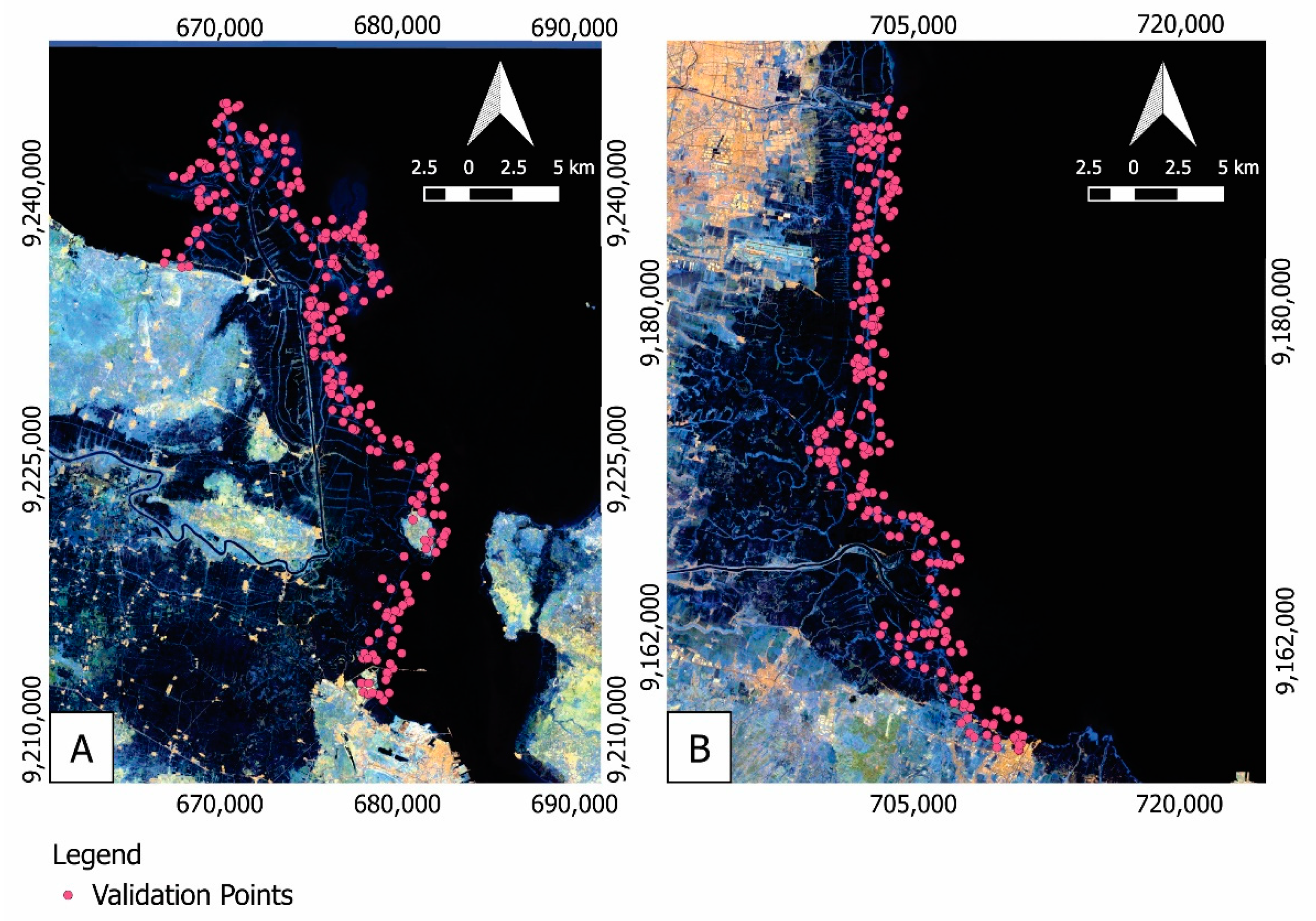
2.1. Study Area
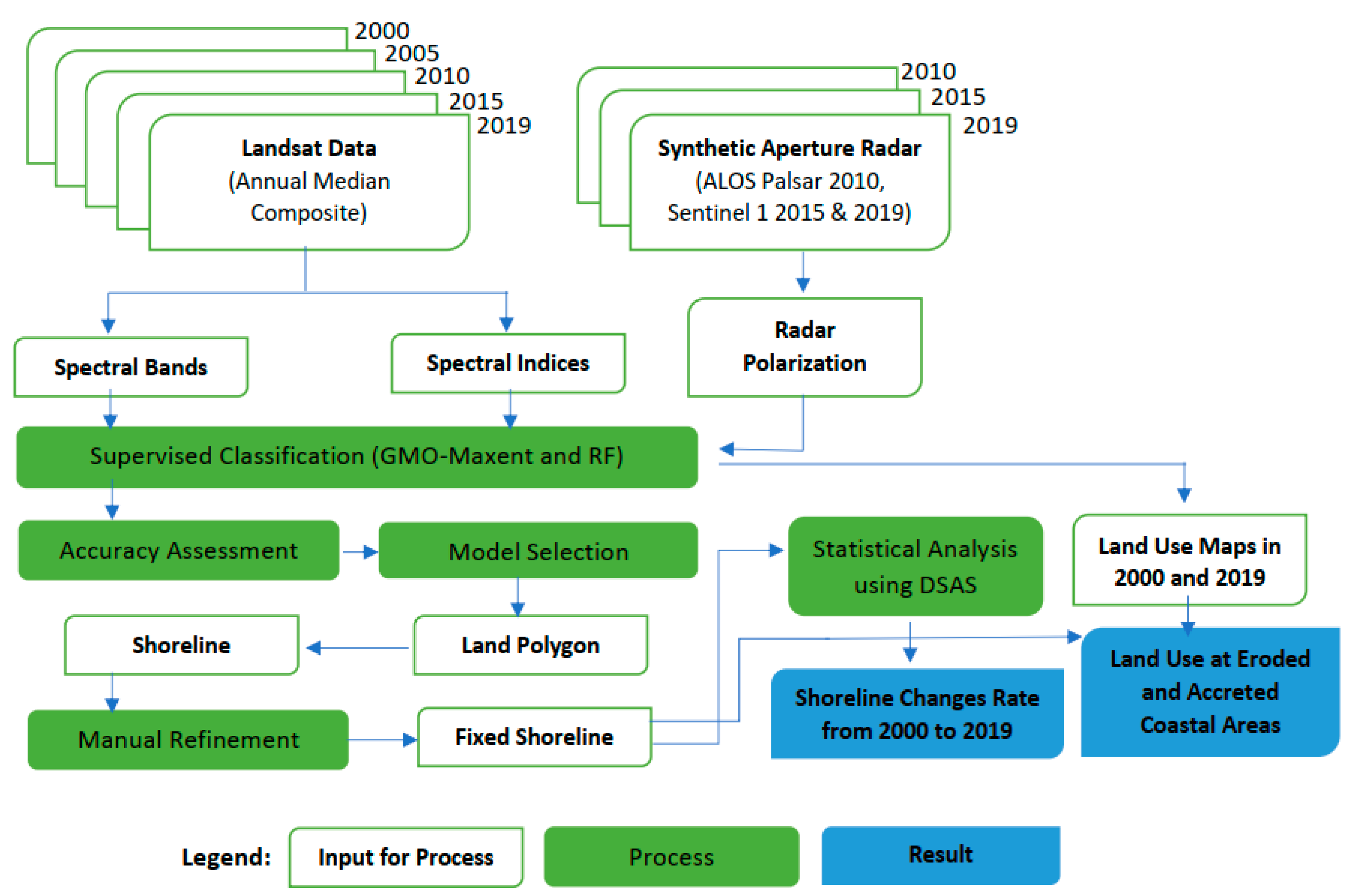
2.2. Data
2.3. Supervised Classification
2.4. Shoreline Refinement and Change Assessment
3. Results
3.1. Accuracy Assessment
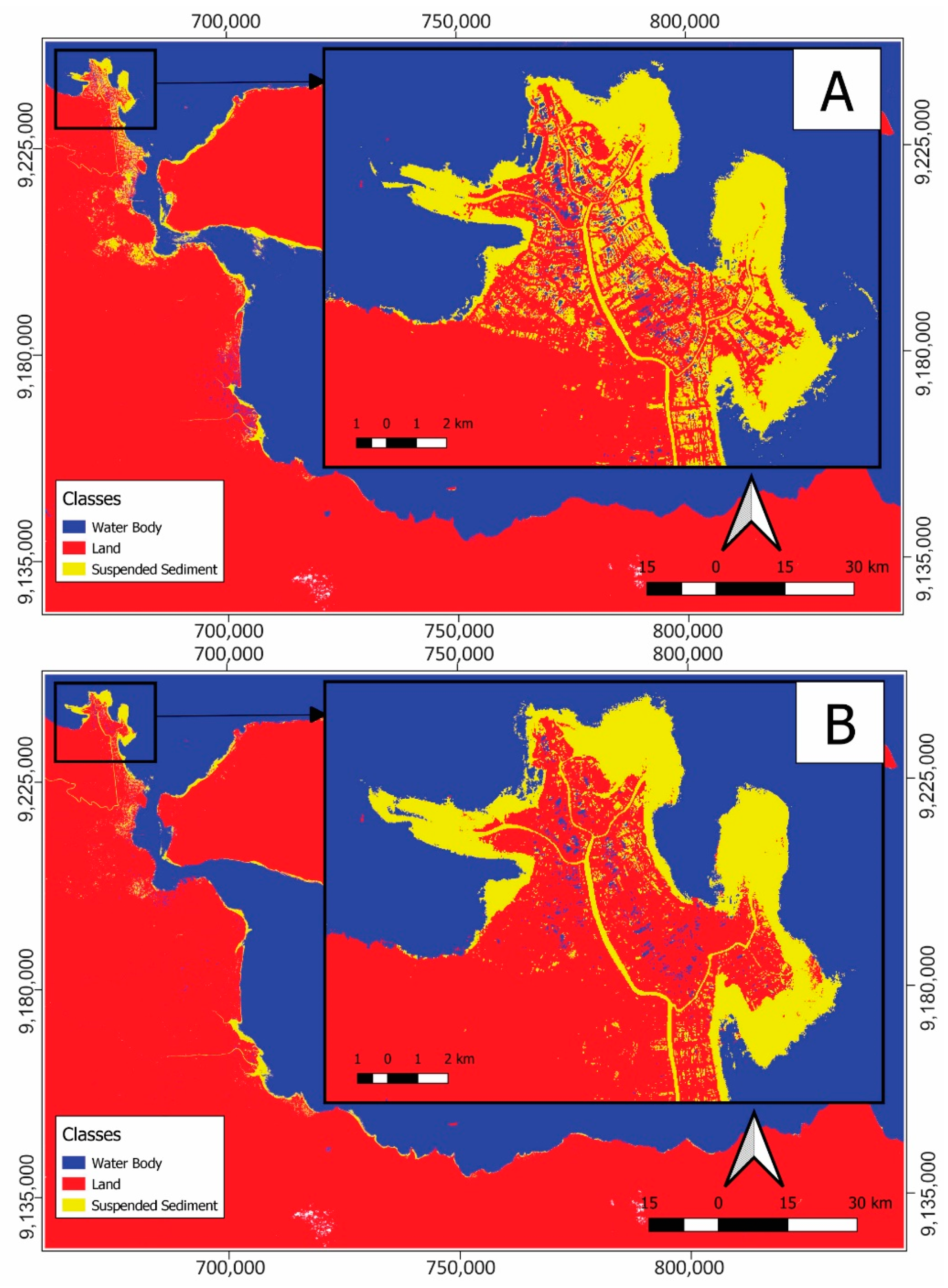
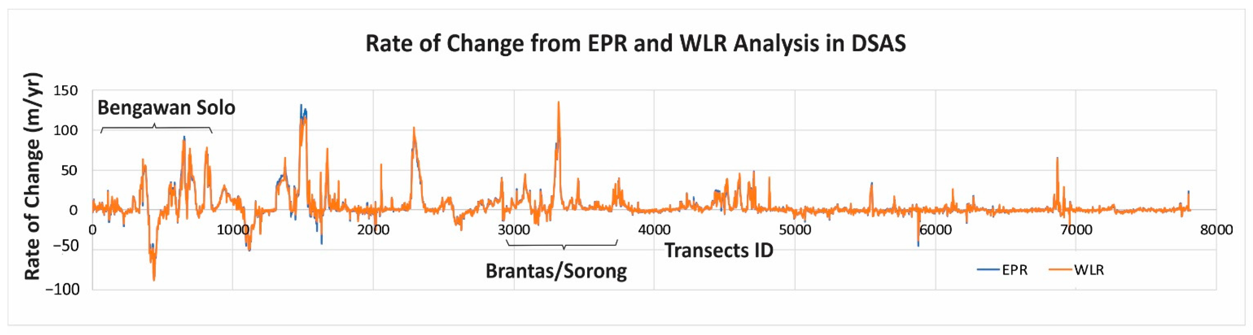
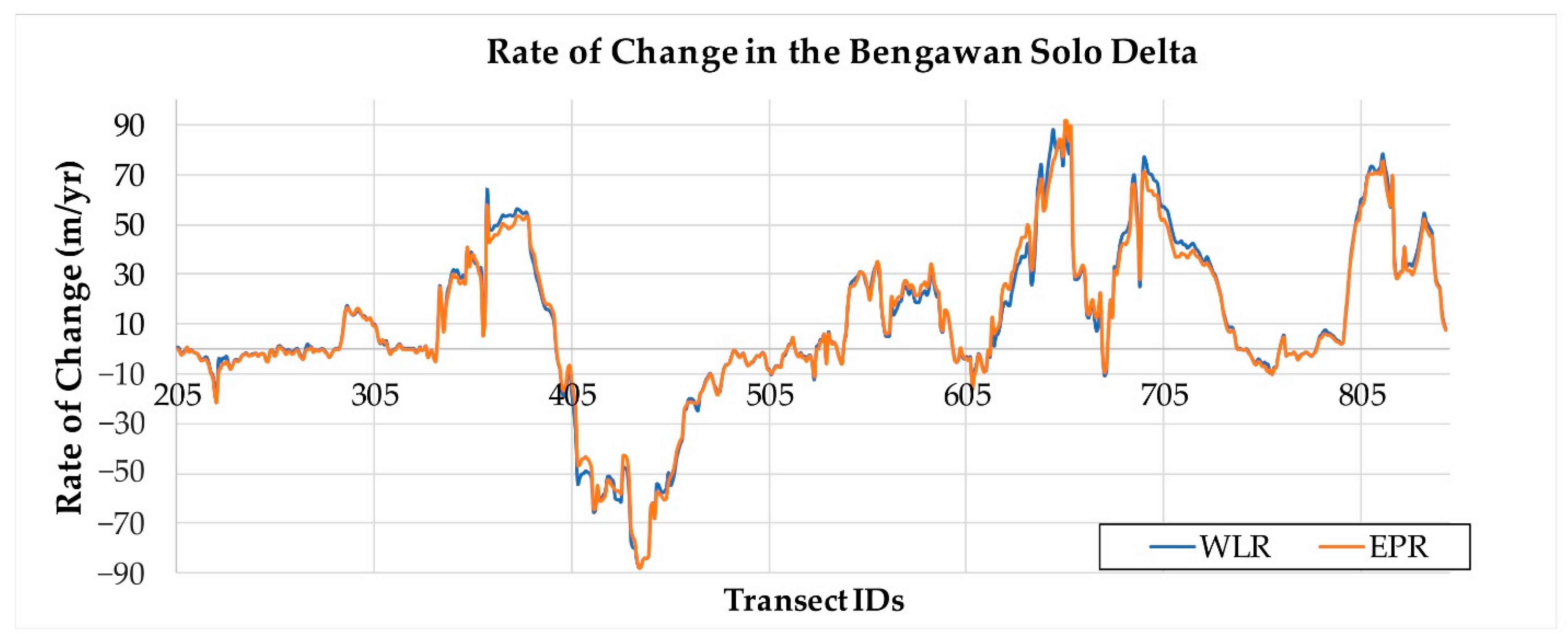
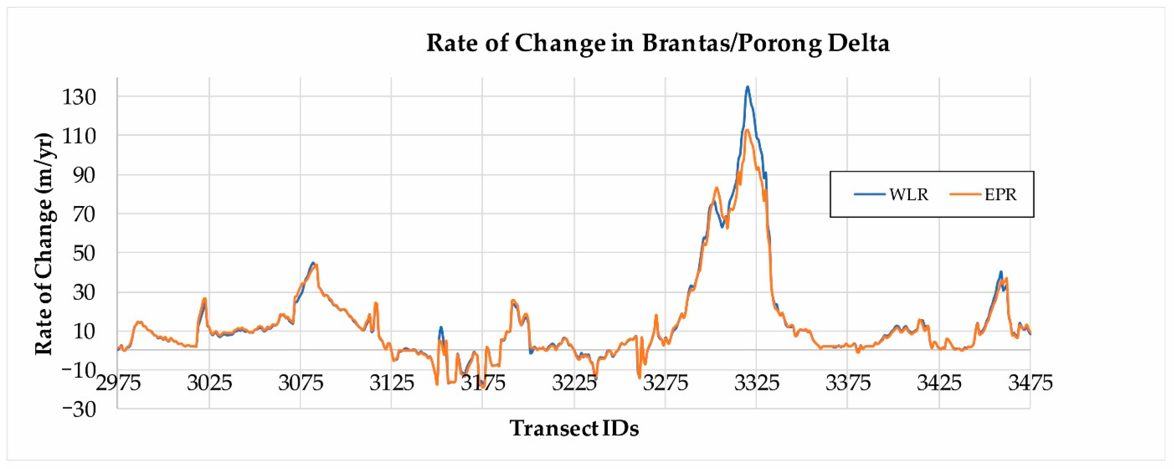
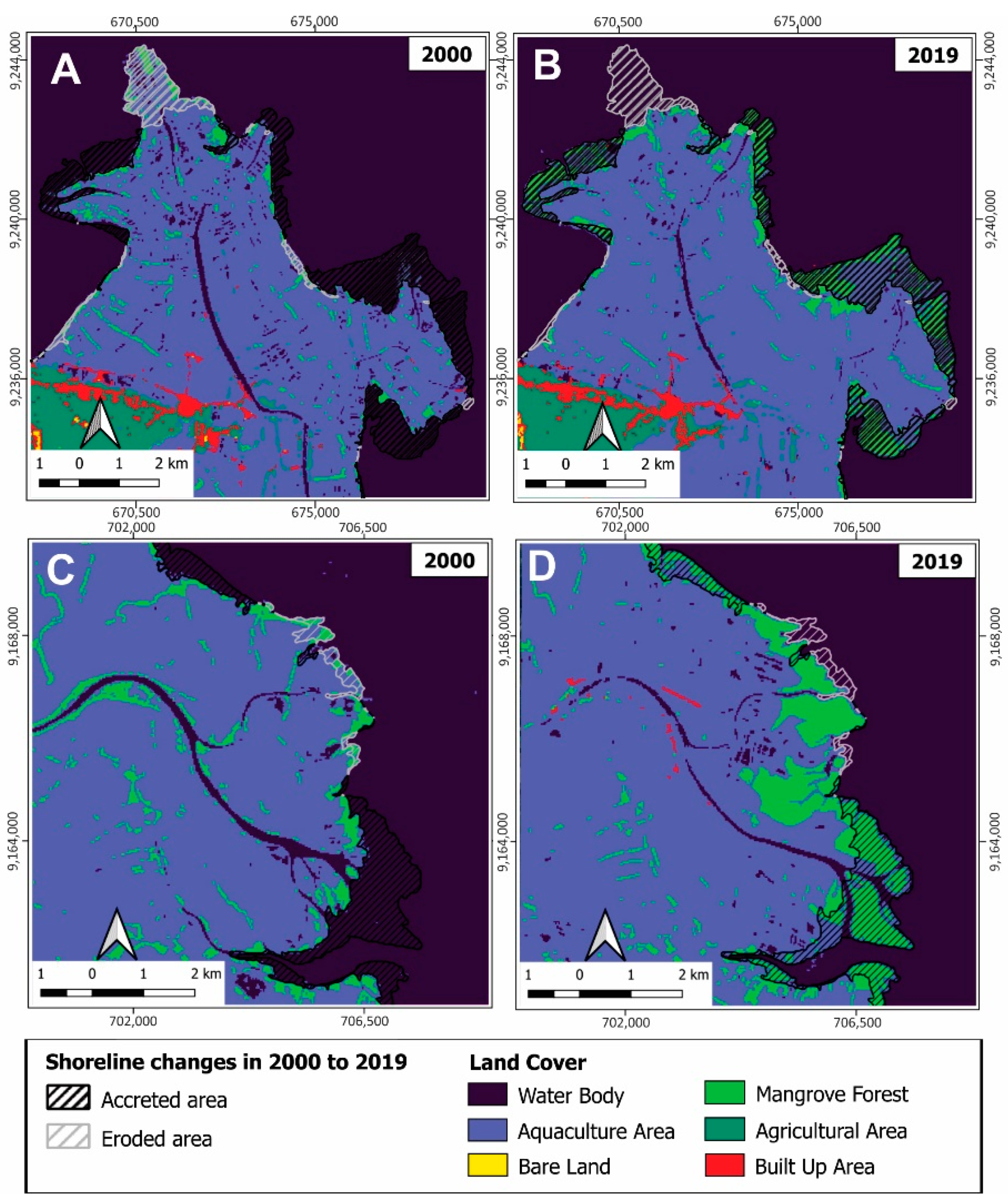
3.2. Shoreline Changes from 2000 to 2019
3.3. Land Use of the Accretion and Erosion Areas in the Coastal Regions in 2000 to 2019
4. Discussion
4.1. Detecting Shorelines from Satellite Imagery Data
4.2. Shoreline and Land-Use Changes from 2000 to 2019
5. Conclusions
Supplementary Materials
Author Contributions
Funding
Institutional Review Board Statement
Informed Consent Statement
Data Availability Statement
Acknowledgments
Conflicts of Interest
References
- Erlandson, J.M. Racing a rising tide: Global warming, rising seas, and the erosion of human history. J. Isl. Coast. Archeol. 2008, 3, 167–169. [Google Scholar] [CrossRef]
- Church, J.A.; White, N.J. A 20th century acceleration in global sea-level rise. Geophys. Res. Lett. 2006, 33. [Google Scholar] [CrossRef]
- Rahmstorf, S. A semi-empirical approach to projecting future sea-level rise. Science 2007, 315, 368–370. [Google Scholar] [CrossRef] [PubMed]
- Nicholls, R.J.; Cazenave, A. Sea-level rise and its impact on coastal zones. Science 2010, 328, 1517–1520. [Google Scholar] [CrossRef] [PubMed]
- Shepherd, A.; Ivins, E.R.; Geruo, A.; Barletta, V.R.; Bentley, M.J.; Bettadpur, S.; Briggs, K.H.; Bromwich, D.H.; Forsberg, R.; Galin, N. A reconciled estimate of ice-sheet mass balance. Science 2012, 338, 1183–1189. [Google Scholar] [CrossRef] [PubMed]
- Everts, C.H. Sea level rise effects on shoreline position. J. Waterw. Port. Coast. Ocean Eng. 1985, 111, 985–999. [Google Scholar] [CrossRef]
- Cazenave, A.; Cozannet, G.L. Sea level rise and its coastal impacts. Earth’s Future 2014, 2, 15–34. [Google Scholar] [CrossRef]
- Leatherman, S.P.; Zhang, K.; Douglas, B.C. Sea level rise shown to drive coastal erosion. Trans. Am. Geophys. Union 2000, 81, 55–57. [Google Scholar] [CrossRef]
- Zhang, K.; Douglas, B.C.; Leatherman, S.P. Global warming and coastal erosion. Clim. Chang. 2004, 64, 41. [Google Scholar] [CrossRef]
- Mutaqin, B.W. Shoreline changes analysis in kuwaru coastal area, Yogyakarta, Indonesia: An application of the digital shoreline analysis system (DSAS). Int. J. Sustain. Dev. Plan. 2017, 12, 1203–1214. [Google Scholar] [CrossRef]
- Ji, T.; Li, G. Contemporary monitoring of storm surge activity. Prog. Phys. Geogr. Earth Environ. 2020, 44, 299–314. [Google Scholar] [CrossRef]
- Lionello, P.; Cavaleri, L.; Nissen, K.M.; Pino, C.; Raicich, F.; Ulbrich, U. Severe marine storms in the Northern Adriatic: Characteristics and trends. Phys. Chem. Earth 2012, 40–41, 93–105. [Google Scholar] [CrossRef]
- Temmerman, S.; Meire, P.; Bouma, T.J.; Herman, P.M.J.; Ysebaert, T.; De Vriend, H.J. Ecosystem-based coastal defence in the face of global change. Nature 2013, 504, 79–83. [Google Scholar] [CrossRef] [PubMed]
- Mentaschi, L.; Vousdoukas, M.I.; Pekel, J.-F.; Voukouvalas, E.; Feyen, L. Global long-term observations of coastal erosion and accretion. Sci. Rep. 2018, 8, 1–11. [Google Scholar] [CrossRef] [PubMed]
- Leatherman, S.P.; Douglas, B.C.; LaBrecque, J.L. Sea level and coastal erosion require large-scale monitoring. Trans. Am. Geophys. Union 2003, 84, 13–16. [Google Scholar] [CrossRef]
- Ingebritsen, S.E.; Galloway, D.L. Coastal subsidence and relative sea level rise. Environ. Res. Lett. 2014, 9, 091002. [Google Scholar] [CrossRef]
- Williams, S.J. Sea-level rise implications for coastal regions. J. Coast. Res. 2013, 184–196. [Google Scholar] [CrossRef]
- Stive, M.J. How important is global warming for coastal erosion? Clim. Chang. 2004, 64, 27. [Google Scholar] [CrossRef]
- Marfai, M.A. The hazards of coastal erosion in Central Java, Indonesia: An overview. Geogr. Malays. J. Soc. Space 2017, 7, 1–9. [Google Scholar]
- Marfai, M.A.; King, L. Coastal flood management in Semarang, Indonesia. Environ. Geol. 2008, 55, 1507–1518. [Google Scholar] [CrossRef]
- Salim, W.; Kombaitan, B.J.C. Jakarta: The rise and challenge of a capital. City 2009, 13, 120–128. [Google Scholar] [CrossRef]
- Martins, G.M.; Amaral, A.F.; Wallenstein, F.M.; Neto, A.I. Influence of a breakwater on nearby rocky intertidal community structure. Mar. Environ. Res. 2009, 67, 237–245. [Google Scholar] [CrossRef] [PubMed]
- Maiolo, M.; Mel, R.A.; Sinopoli, S. A Stepwise Approach to Beach Restoration at Calabaia Beach. Water 2020, 12, 2677. [Google Scholar] [CrossRef]
- Ye, G.; Chou, L.M.; Yang, S.; Wu, J.; Liu, P.; Jin, C. Is integrated coastal management an effective framework for promoting coastal sustainability in China’s coastal cities? Mar. Policy 2015, 56, 48–55. [Google Scholar] [CrossRef]
- Turner, R.K. Integrating natural and socio-economic science in coastal management. J. Mar. Syst. 2000, 25, 447–460. [Google Scholar] [CrossRef]
- Marfai, M.A.; Almohammad, H.; Dey, S.; Susanto, B.; King, L. Coastal dynamic and shoreline mapping: Multi-sources spatial data analysis in Semarang Indonesia. Environ. Monit. Assess. 2008, 142, 297–308. [Google Scholar] [CrossRef]
- Libriyono, A.; Kusratmoko, E.; Kertopermono, A.P. Spatial modelling of shoreline change to coastal disaster management in Jakarta Bay. AIP Conf. Proc. 2018, 1987, 020021. [Google Scholar]
- Chairani, C.; Saraswati, R.; Shidiq, I. Identification of changes mangrove areas toward shoreline changes in East Coast of Surabaya 2004–2017. In Proceedings of the IOP Conference Series: Earth and Environmental Science, Bandung, Indonesia, 2–4 July 2018; p. 012002. [Google Scholar]
- Fuad, M.; Fais, D. Automatic Detection of Decadal Shoreline Change on Northern Coastal of Gresik, East Java-Indonesia. In Proceedings of the IOP Conference Series: Earth and Environmental Science, Yogyakarta, Indonesia, 27–28 September 2017. [Google Scholar]
- Dewi, R.S.; Bijker, W.; Stein, A.; Marfai, M.A. Fuzzy classification for shoreline change monitoring in a part of the northern coastal area of Java, Indonesia. Remote Sens. 2016, 8, 190. [Google Scholar] [CrossRef]
- Blodget, H.; Taylor, P.; Roark, J. Shoreline changes along the Rosetta-Nile Promontory: Monitoring with satellite observations. Mar. Geol. 1991, 99, 67–77. [Google Scholar] [CrossRef]
- Kuleli, T. Quantitative analysis of shoreline changes at the Mediterranean Coast in Turkey. Environ. Monit. Assess. 2010, 167, 387–397. [Google Scholar] [CrossRef]
- Tamassoki, E.; Amiri, H.; Soleymani, Z. Monitoring of shoreline changes using remote sensing (case study: Coastal city of Bandar Abbas). In Proceedings of the IOP Conference Series: Earth and Environmental Science, Kuala Lumpur, Malaysia, 22–23 April 2014; p. 012023. [Google Scholar]
- Thi, V.T.; Xuan, A.T.T.; Nguyen, H.P.; Dahdouh-Guebas, F.; Koedam, N. Application of remote sensing and GIS for detection of long-term mangrove shoreline changes in Mui Ca Mau, Vietnam. Biogeosciences 2014, 11, 3781. [Google Scholar]
- M-Muslim, A.; Foody, G.M.; Atkinson, P.M. Shoreline mapping from coarse–spatial resolution remote sensing imagery of Seberang Takir, Malaysia. J. Coast. Res. 2007, 23, 1399–1408. [Google Scholar] [CrossRef]
- Gorelick, N.; Hancher, M.; Dixon, M.; Ilyushchenko, S.; Thau, D.; Moore, R. Google Earth Engine: Planetary-scale geospatial analysis for everyone. Remote Sens. Environ. 2017, 202, 18–27. [Google Scholar] [CrossRef]
- Chu, L.; Oloo, F.; Sudmanns, M.; Tiede, D.; Hölbling, D.; Blaschke, T.; Teleoaca, I. Monitoring long-term shoreline dynamics and human activities in the Hangzhou Bay, China, combining daytime and nighttime EO data. Big Earth Data 2020, 4, 1–23. [Google Scholar] [CrossRef]
- Vos, K.; Harley, M.D.; Splinter, K.D.; Simmons, J.A.; Turner, I.L. Sub-annual to multi-decadal shoreline variability from publicly available satellite imagery. Coast. Eng. 2019, 150, 160–174. [Google Scholar] [CrossRef]
- Propp, C.; Jänen, I.; Jennerjahn, T. Sources and degradation of sedimentary organic matter in coastal waters off the Brantas River, Java, Indonesia. Asian J. Water Environ. Pollut. 2013, 10, 95–115. [Google Scholar]
- Lebreton, L.C.; Van Der Zwet, J.; Damsteeg, J.-W.; Slat, B.; Andrady, A.; Reisser, J. River plastic emissions to the world’s oceans. Nat. Commun. 2017, 8, 15611. [Google Scholar] [CrossRef]
- Lestari, P.; Trihadiningrum, Y.; Wijaya, B.A.; Yunus, K.A.; Firdaus, M. Distribution of microplastics in Surabaya River, Indonesia. Sci. Total Environ. 2020, 726, 138560. [Google Scholar] [CrossRef]
- Lestari, P.; Trihadiningrum, Y. The impact of improper solid waste management to plastic pollution in Indonesian coast and marine environment. Mar. Pollut. Bull. 2019, 149, 110505. [Google Scholar] [CrossRef]
- Wang, Y.C.; Feng, C.C.; Vu Duc, H. Integrating Multi-Sensor Remote Sensing Data for Land Use/Cover Mapping in a Tropical Mountainous Area in Northern Thailand. Geogr. Res. 2012, 50, 320–331. [Google Scholar] [CrossRef]
- Töyrä, J.; Pietroniro, A.; Martz, L.W.; Prowse, T.D. A multi-sensor approach to wetland flood monitoring. Hydrol. Process. 2002, 16, 1569–1581. [Google Scholar] [CrossRef]
- Taha, L.G.E.-d.; Elbeih, S.F. Investigation of fusion of SAR and Landsat data for shoreline super resolution mapping: The northeastern Mediterranean Sea coast in Egypt. Appl. Geomat. 2010, 2, 177–186. [Google Scholar] [CrossRef]
- McFeeters, S.K. The use of the Normalized Difference Water Index (NDWI) in the delineation of open water features. Int. J. Remote Sens. 1996, 17, 1425–1432. [Google Scholar] [CrossRef]
- JW, R.; Haas, R.; Schell, J.; Deering, D. Monitoring vegetation systems in the Great Plains with ERTS. In Proceedings of the Third Earth Resources Technology Satellite-1 Symposium, Washington, DC, USA, 10–14 December 1973; Volume 1, pp. 309–317. [Google Scholar]
- Feyisa, G.L.; Meilby, H.; Fensholt, R.; Proud, S.R. Automated Water Extraction Index: A new technique for surface water mapping using Landsat imagery. Remote Sens. Environ. 2014, 140, 23–35. [Google Scholar] [CrossRef]
- Mcdonald, R.; Mohri, M.; Silberman, N.; Walker, D.; Mann, G.S. Efficient large-scale distributed training of conditional maximum entropy models. Adv. Neural Inf. Process. Syst. 2009, 22, 1231–1239. [Google Scholar]
- Segal, I.E. A note on the concept of entropy. J. Math. Mech. 1948, 27, 379–423. [Google Scholar] [CrossRef]
- Vajapeyam, S. Understanding Shannon’s Entropy metric for Information. arXiv 2014, arXiv:1405.2061. [Google Scholar]
- Jaynes, E.T. Information theory and statistical mechanics. Phys. Rev. 1957, 106, 620. [Google Scholar] [CrossRef]
- Phillips, S.J.; Anderson, R.P.; Schapire, R.E. Maximum entropy modeling of species geographic distributions. Ecol. Model. 2006, 190, 231–259. [Google Scholar] [CrossRef]
- Phillips, S.J.; Dudík, M.; Schapire, R.E. A maximum entropy approach to species distribution modeling. In Proceedings of the Twenty-First International Conference on Machine Learning, Banff, Alberta, 4–8 July 2004; p. 83. [Google Scholar]
- Ahmed, N.; Islam, M.N.; Hasan, M.F.; Motahar, T.; Sujauddin, M. Understanding the political ecology of forced migration and deforestation through a multi-algorithm classification approach: The case of Rohingya displacement in the southeastern border region of Bangladesh. Geol. Ecol. Landsc. 2019, 3, 282–294. [Google Scholar] [CrossRef]
- Baldwin, R.A. Use of maximum entropy modeling in wildlife research. Entropy 2009, 11, 854–866. [Google Scholar] [CrossRef]
- Kumar, S.; Stohlgren, T.J. Maxent modeling for predicting suitable habitat for threatened and endangered tree Canacomyrica monticola in New Caledonia. J. Ecol. Nat. Environ. 2009, 1, 094–098. [Google Scholar]
- Li, W.; Guo, Q. A maximum entropy approach to one-class classification of remote sensing imagery. Int. J. Remote Sens. 2010, 31, 2227–2235. [Google Scholar] [CrossRef]
- Breiman, L. Random forests. Mach. Learn. 2001, 45, 5–32. [Google Scholar] [CrossRef]
- Himmelstoss, E.A.; Henderson, R.E.; Kratzmann, M.G.; Farris, A.S. Digital Shoreline Analysis System (DSAS) Version 5.0 User Guide; US Geological Survey: Reston, VA, USA, 2018; pp. 1258–2331.
- Baig, M.R.I.; Ahmad, I.A.; Shahfahad; Tayyab, M.; Rahman, A. Analysis of shoreline changes in Vishakhapatnam coastal tract of Andhra Pradesh, India: An application of digital shoreline analysis system (DSAS). Ann. Gis. 2020, 26, 361–376. [Google Scholar] [CrossRef]
- Thinh, N.A.; Hens, L. A Digital Shoreline Analysis System (DSAS) applied on mangrove shoreline changes along the Giao Thuy coastal area (Nam Dinh, Vietnam) during 2005–2014. Vietnam J. Earth Sci. 2017, 39, 87–96. [Google Scholar] [CrossRef]
- Maryantika, N.; Lin, C. Exploring changes of land use and mangrove distribution in the economic area of Sidoarjo District, East Java using multi-temporal Landsat images. Inf. Process. Agric. 2017, 4, 321–332. [Google Scholar] [CrossRef]
- Alesheikh, A.A.; Ghorbanali, A.; Nouri, N. Coastline change detection using remote sensing. Int. J. Environ. Sci. Technol. 2007, 4, 61–66. [Google Scholar] [CrossRef]
- Sunder, S.; Ramsankaran, R.; Ramakrishnan, B. Inter-comparison of remote sensing sensing-based shoreline mapping techniques at different coastal stretches of India. Environ. Monit. Assess. 2017, 189, 290. [Google Scholar] [CrossRef]
- Kelly, J.T.; Gontz, A.M. Using GPS-surveyed intertidal zones to determine the validity of shorelines automatically mapped by Landsat water indices. Int. J. Appl. Earth Obs. Geoinf. 2018, 65, 92–104. [Google Scholar] [CrossRef]
- Masria, A.; Nadaoka, K.; Negm, A.; Iskander, M.J.L. Detection of shoreline and land cover changes around Rosetta promontory, Egypt, based on remote sensing analysis. Land 2015, 4, 216–230. [Google Scholar] [CrossRef]
- Sekovski, I.; Stecchi, F.; Mancini, F.; Del Rio, L. Image classification methods applied to shoreline extraction on very high-resolution multispectral imagery. Int. J. Remote Sens. 2014, 35, 3556–3578. [Google Scholar] [CrossRef]
- Wicaksono, A.; Wicaksono, P. Geometric Accuracy Assessment for Shoreline Derived from NDWI, MNDWI, and AWEI Transformation on Various Coastal Physical Typology in Jepara Regency using Landsat 8 OLI Imagery in 2018. Geoplanning J. Geomat. Plan. 2019, 6, 55–72. [Google Scholar] [CrossRef]
- Farda, N. Multi-temporal land use mapping of coastal wetlands area using machine learning in Google earth engine. In Proceedings of the IOP Conference Series: Earth and Environmental Science, Yogyakarta, Indonesia, 27–28 September 2017; p. 012042. [Google Scholar]
- Shelestov, A.; Lavreniuk, M.; Kussul, N.; Novikov, A.; Skakun, S. Exploring Google Earth Engine platform for big data processing: Classification of multi-temporal satellite imagery for crop mapping. Front. Earth Sci. 2017, 5, 17. [Google Scholar] [CrossRef]
- Kure, S.; Winarta, B.; Takeda, Y.; Udo, K.; Umeda, M.; Mano, A.; Tanaka, H. Effects of mud flows from the LUSI mud volcano on the Porong River estuary, Indonesia. J. Coast. Res. 2014, 568–573. [Google Scholar] [CrossRef]
- Wijayanti, N.D. Pemetaan distribusi total suspended solid dan perubahan garis pantai di sidoarjo-pasuruan dengan menggunakan data penginderaan jauh. Geomatika 2020, 26, 25–34. [Google Scholar] [CrossRef]
- Hoekstra, P. The development of two major Indonesian river deltas: Morphology and sedimentary aspects of the Solo and Porong delta, East Java. In Coastal Lowlands; Springer: Dordrecht, The Netherlands, 1989; pp. 143–159. [Google Scholar]
- Hoekstra, P.; Tiktanaka. Coastal hydrodynamics, geomorphology and sedimentary environments of two major Javanese river deltas. Program and preliminary results from the Snellius-II expedition (Indonesia). J. Southeast Asian Earth Sci. 1988, 2, 95–107. [Google Scholar] [CrossRef]
- Van Wesenbeeck, B.; Balke, T.; Van Eijk, P.; Tonneijck, F.; Siry, H.; Rudianto, M.; Winterwerp, J. Aquaculture induced erosion of tropical coastlines throws coastal communities back into poverty. Ocean Coast. Manag. 2015, 116, 466–469. [Google Scholar] [CrossRef]
- Dharmawan, B.; Böcher, M.; Krott, M. Endangered mangroves in Segara Anakan, Indonesia: Effective and failed problem-solving policy advice. Environ. Manag. 2017, 60, 409–421. [Google Scholar] [CrossRef]
- Perry, C.T.; Smithers, S.G.; Gulliver, P.; Browne, N.K. Evidence of very rapid reef accretion and reef growth under high turbidity and terrigenous sedimentation. Geology 2012, 40, 719–722. [Google Scholar] [CrossRef]
- Satta, A.; Puddu, M.; Venturini, S.; Giupponi, C. Assessment of coastal risks to climate change related impacts at the regional scale: The case of the Mediterranean region. Int. J. Disaster Risk Reduct. 2017, 24, 284–296. [Google Scholar] [CrossRef]
- Gornitz, V.M.; Daniels, R.C.; White, T.W.; Birdwell, K.R. The development of a coastal risk assessment database: Vulnerability to sea-level rise in the US Southeast. J. Coast. Res. 1994, 12, 327–338. [Google Scholar]


| Year of Analysis | Sensors | Input Band |
|---|---|---|
| 2000 | Landsat-7 ETM+ (SR) | red, green, blue, NIR, SWIR1, SWIR2 |
| NDWI, NDVI, AWEInsh | ||
| 2005 | Landsat-7 ETM+ (SR) | red, green, blue, NIR, SWIR1, SWIR2 |
| NDWI, NDVI, AWEInsh | ||
| 2010 | Landsat-7 ETM+ (SR) | red, green, blue, NIR, SWIR1, SWIR2 |
| NDWI, NDVI, AWEInsh | ||
| Alos PALSAR/Global Palsar | HH, HV | |
| 2015 | Landsat-8 OLI (T1_SR) | red, green, blue, NIR, SWIR1, SWIR2 |
| NDWI, NDVI, AWEInsh | ||
| Sentinel-1 Descending Orbit | VV, VH | |
| 2019 | Landsat-8 OLI (T1_SR) | red, green, blue, NIR, SWIR1, SWIR2 |
| NDWI, NDVI, AWEInsh | ||
| Sentinel-1 Descending Orbit | VV, VH |
| 2000 | |||||||||
| Class | RF (ntree: 50) | RF (ntree: 80) | GMO-Maxent | ||||||
| UA | PA | OA | UA | PA | OA | UA | PA | OA | |
| Land | 78.36 | 94.47 | 84 | 78.18 | 94.86 | 84 | 92.34 | 95.26 | 93.6 |
| Water | 92.82 | 73.28 | 93.26 | 72.87 | 94.98 | 91.90 | |||
| 2005 | |||||||||
| Class | RF (ntree: 50) | RF (ntree: 80) | GMO-Maxent | ||||||
| UA | PA | OA | UA | PA | OA | UA | PA | OA | |
| Land | 81.50 | 94.54 | 84.6 | 80.61 | 89.08 | 84.4 | 86.54 | 94.54 | 90.4 |
| Water | 87.40 | 86.64 | 89.03 | 80.53 | 94.58 | 86.64 | |||
| 2010 | |||||||||
| Class | RF (ntree: 50) | RF (ntree: 80) | GMO-Maxent | ||||||
| UA | PA | OA | UA | PA | OA | UA | PA | OA | |
| Land | 93.65 | 90.42 | 91.8 | 93.68 | 90.80 | 92 | 98.77 | 91.95 | 95.2 |
| Water | 89.92 | 93.31 | 90.28 | 93.31 | 91.83 | 98.74 | |||
| 2015 | |||||||||
| Class | RF (ntree: 50) | RF (ntree: 80) | GMO-Maxent | ||||||
| UA | PA | OA | UA | PA | OA | UA | PA | OA | |
| Land | 90.23 | 89.19 | 89.4 | 88.68 | 90.73 | 89.2 | 84.67 | 85.33 | 84 |
| Water | 88.52 | 89.63 | 89.79 | 87.55 | 84.68 | 82.57 | |||
| 2019 | |||||||||
| Class | RF (ntree: 50) | RF (ntree: 80) | GMO-Maxent | ||||||
| UA | PA | OA | UA | PA | OA | UA | PA | OA | |
| Land | 91.53 | 91.14 | 91.8 | 92.27 | 90.72 | 92 | 90.12 | 92.41 | 91.6 |
| Water | 92.05 | 92.40 | 91.76 | 93.16 | 93.36 | 90.87 | |||
| Delta | Type of Coastal Land | Type of Land Use | Area (ha) |
|---|---|---|---|
| Bengawan Solo | Accreted area in 2019 | Mangrove | 413.44 |
| Aquaculture | 471.50 | ||
| Eroded area in 2019 | Mangrove | 40.05 | |
| Aquaculture | 176.59 | ||
| Brantas/Porong | Accreted area in 2019 | Mangrove | 251.85 |
| Aquaculture | 166.97 | ||
| Eroded area in 2019 | Mangrove | 15.96 | |
| Aquaculture | 41.44 |
Publisher’s Note: MDPI stays neutral with regard to jurisdictional claims in published maps and institutional affiliations. |
© 2021 by the authors. Licensee MDPI, Basel, Switzerland. This article is an open access article distributed under the terms and conditions of the Creative Commons Attribution (CC BY) license (http://creativecommons.org/licenses/by/4.0/).
Share and Cite
Arjasakusuma, S.; Kusuma, S.S.; Saringatin, S.; Wicaksono, P.; Mutaqin, B.W.; Rafif, R. Shoreline Dynamics in East Java Province, Indonesia, from 2000 to 2019 Using Multi-Sensor Remote Sensing Data. Land 2021, 10, 100. https://doi.org/10.3390/land10020100
Arjasakusuma S, Kusuma SS, Saringatin S, Wicaksono P, Mutaqin BW, Rafif R. Shoreline Dynamics in East Java Province, Indonesia, from 2000 to 2019 Using Multi-Sensor Remote Sensing Data. Land. 2021; 10(2):100. https://doi.org/10.3390/land10020100
Chicago/Turabian StyleArjasakusuma, Sanjiwana, Sandiaga Swahyu Kusuma, Siti Saringatin, Pramaditya Wicaksono, Bachtiar Wahyu Mutaqin, and Raihan Rafif. 2021. "Shoreline Dynamics in East Java Province, Indonesia, from 2000 to 2019 Using Multi-Sensor Remote Sensing Data" Land 10, no. 2: 100. https://doi.org/10.3390/land10020100
APA StyleArjasakusuma, S., Kusuma, S. S., Saringatin, S., Wicaksono, P., Mutaqin, B. W., & Rafif, R. (2021). Shoreline Dynamics in East Java Province, Indonesia, from 2000 to 2019 Using Multi-Sensor Remote Sensing Data. Land, 10(2), 100. https://doi.org/10.3390/land10020100