
Sub-Watershed Parameter Transplantation Method for Non-Point Source Pollution Estimation in Complex Underlying Surface Environment

 , , and
Abstract
1. Introduction
2. Materials and Methods
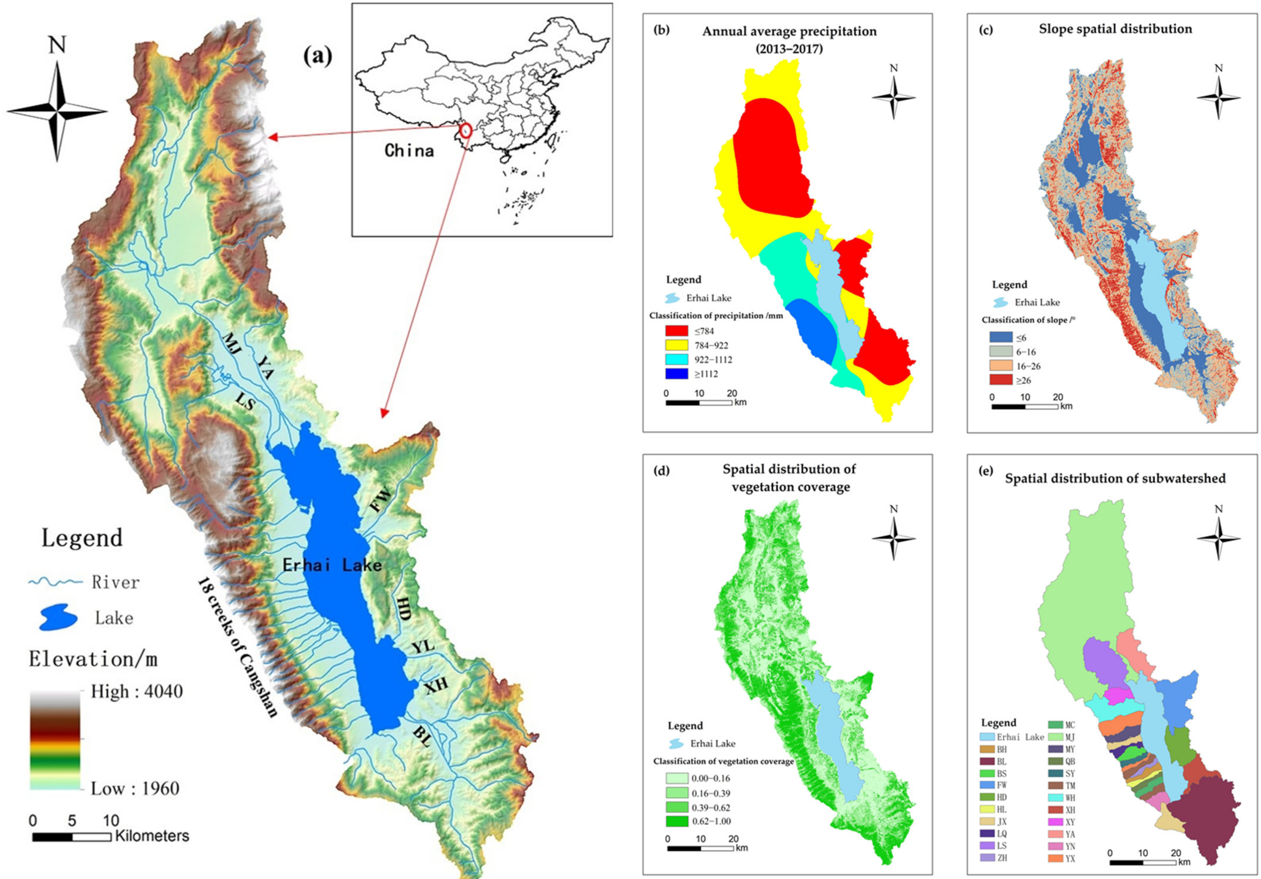
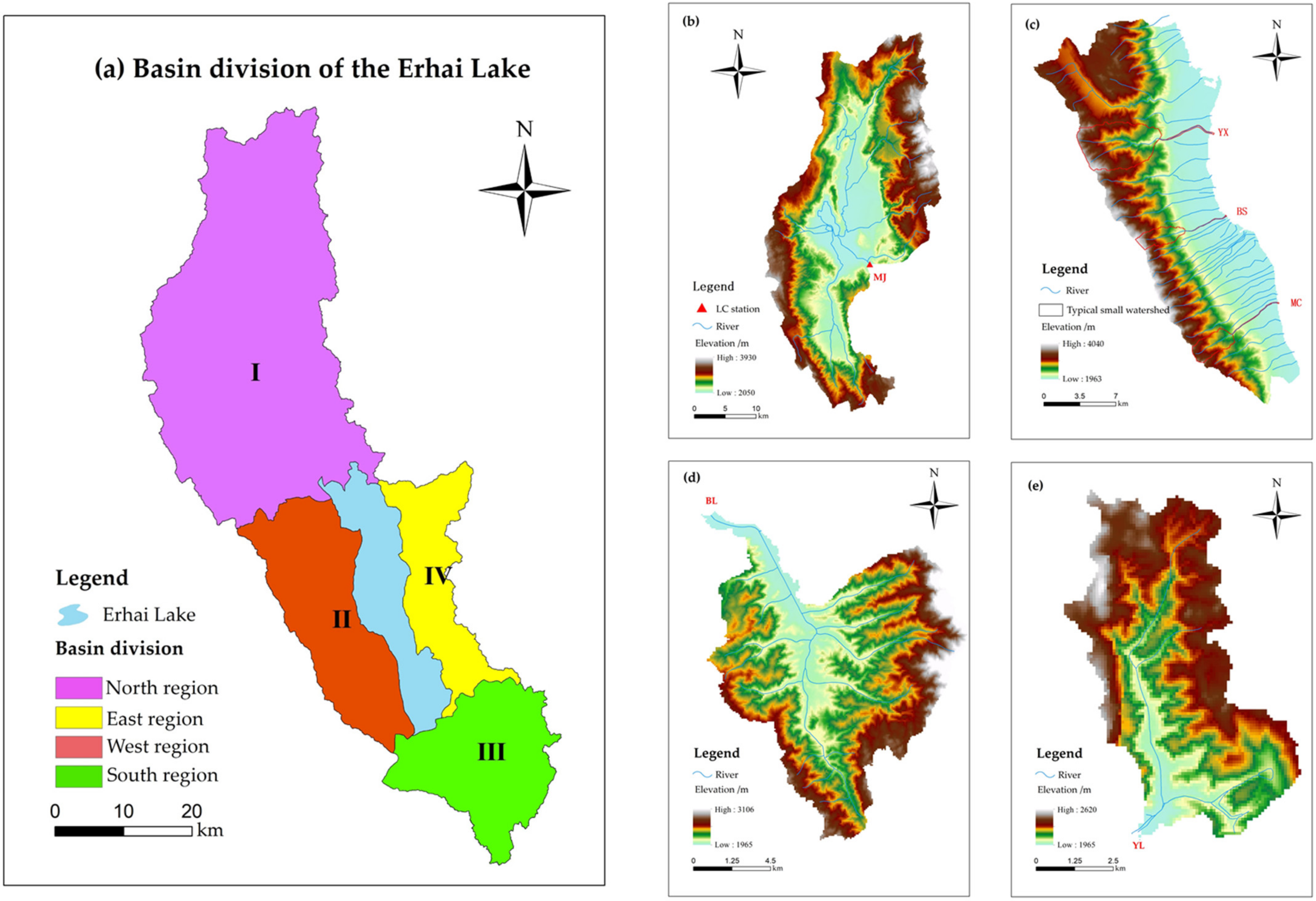
2.1. Study Area and Date Availability
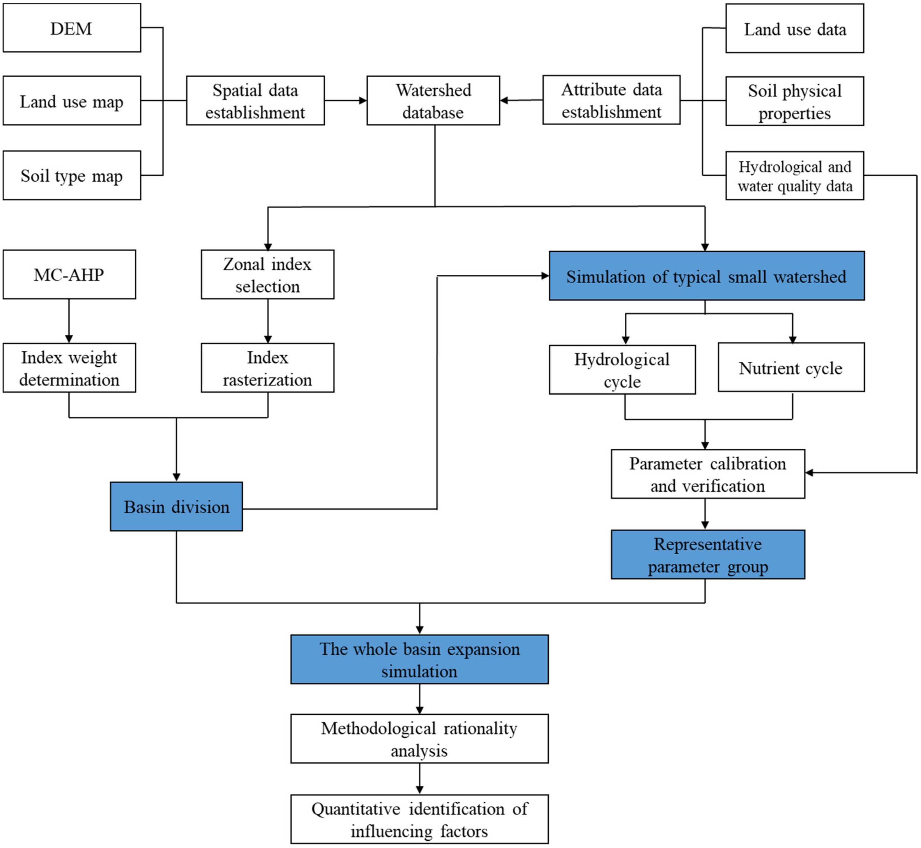
2.2. Sub-Watershed Parameter Transplantation (SWPT)
2.2.1. Dividing Index
2.2.2. Watershed Delineation
2.2.3. Mechanism Model
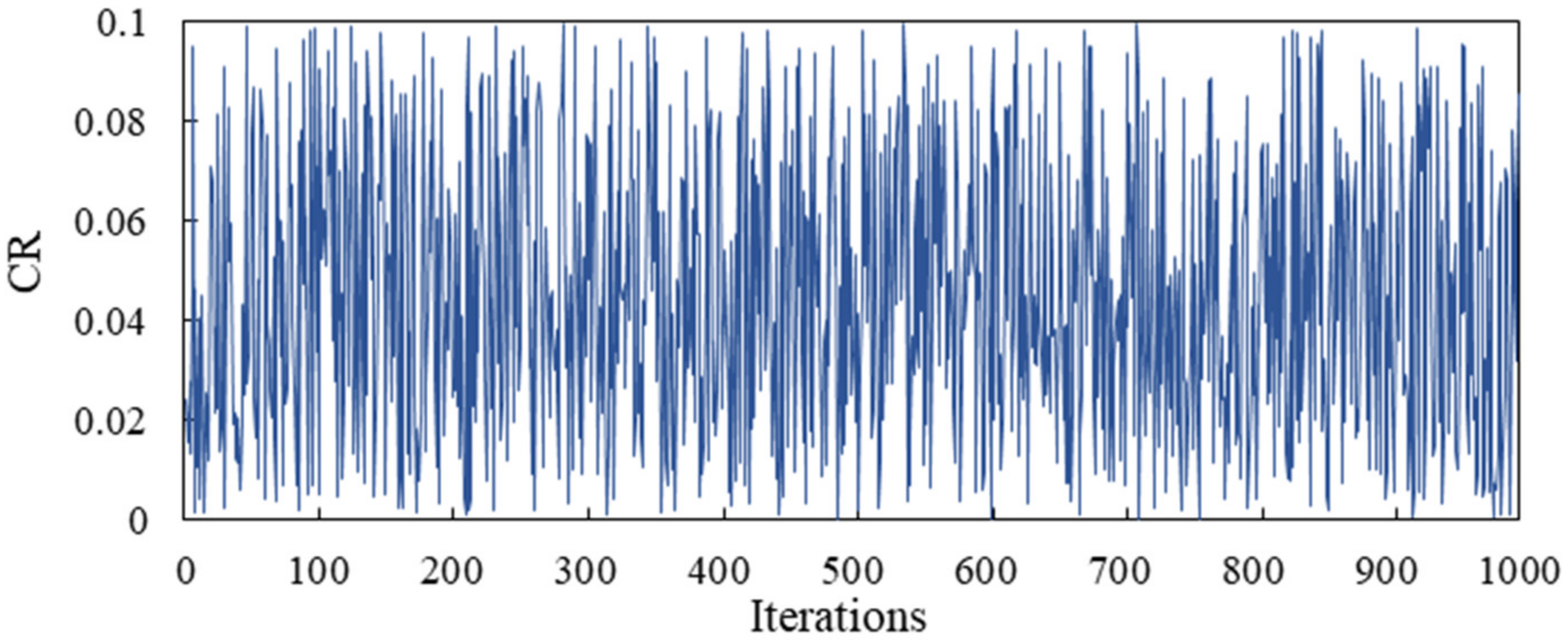
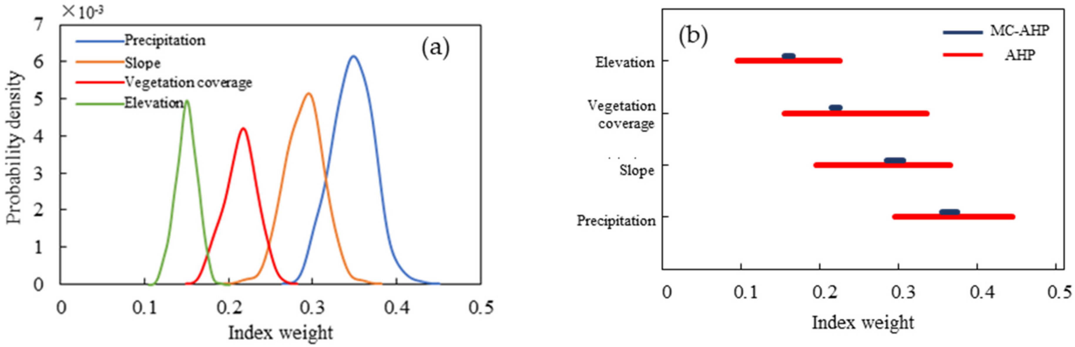
2.3. Monte-Carlo-Based AHP Algorithm (MCAHP)
3. Results and Analysis
3.1. Determination of Weight of Dividing Index
3.2. Watershed Division and Selection of Sub-Watersheds
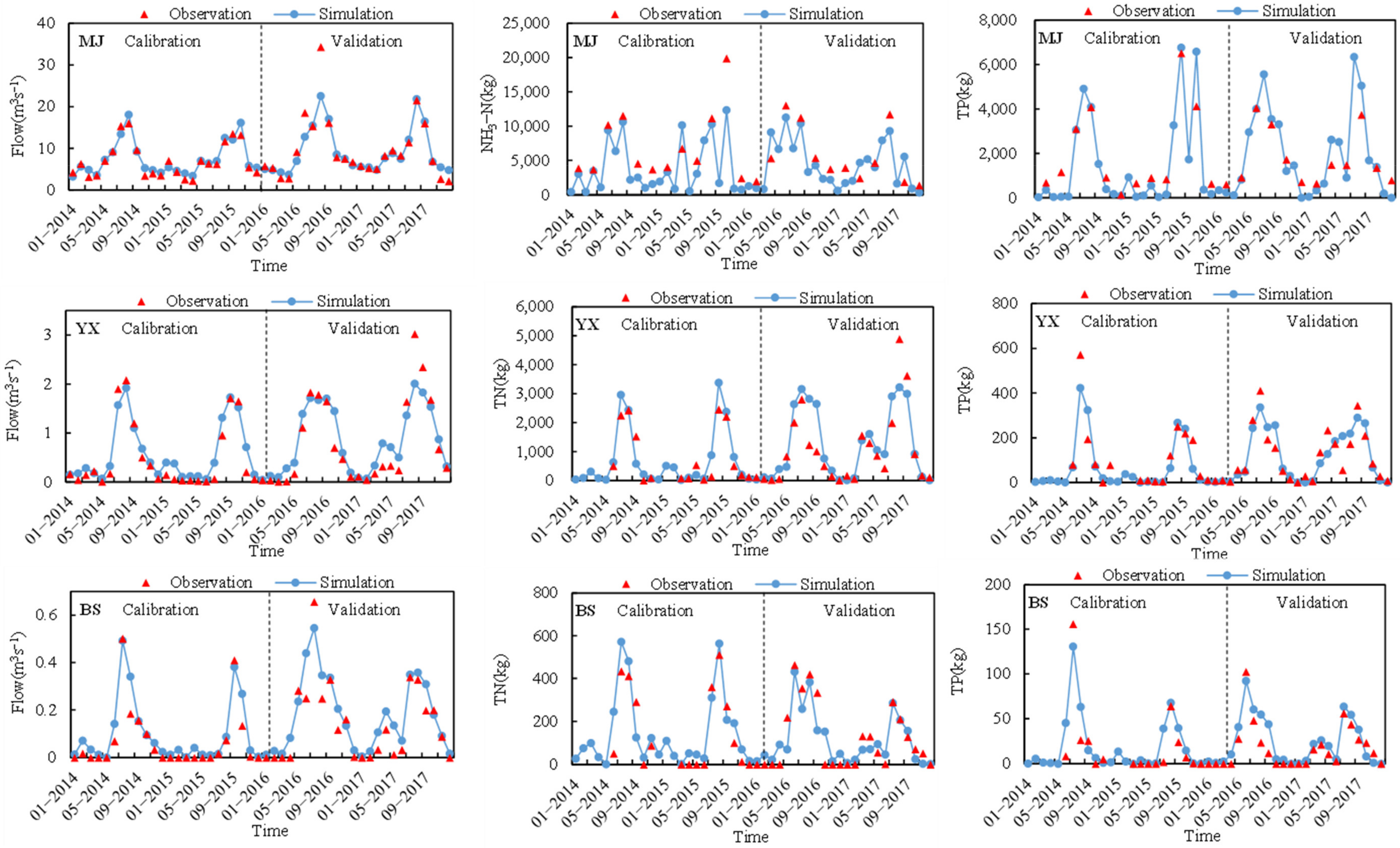
3.3. Simulation of the Sub-Watersheds
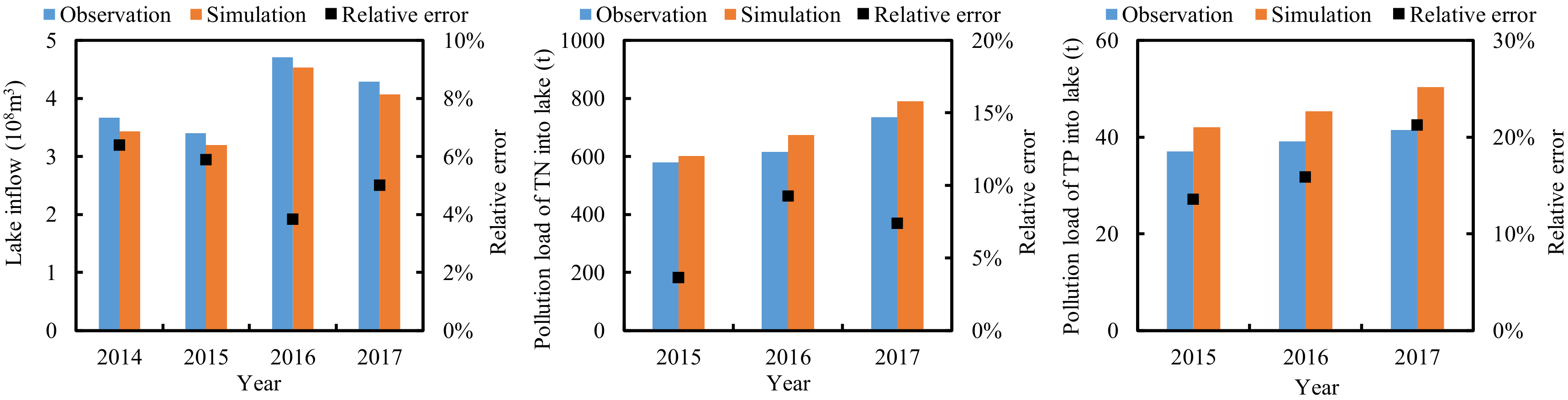
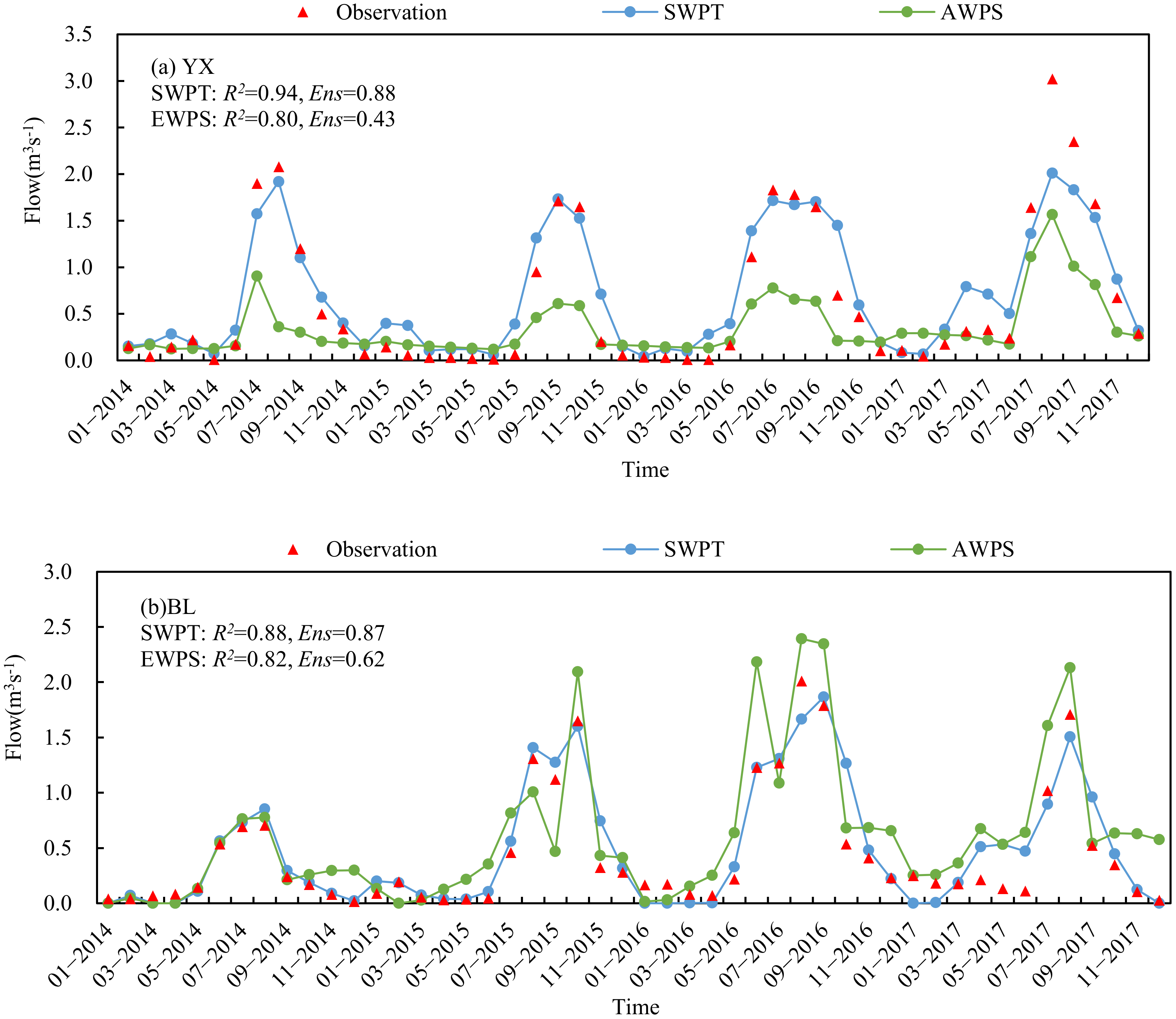
3.4. Extended Simulation
4. Discussion
4.1. Rationality Analysis of the Method
4.2. Identification of Influencing Factors
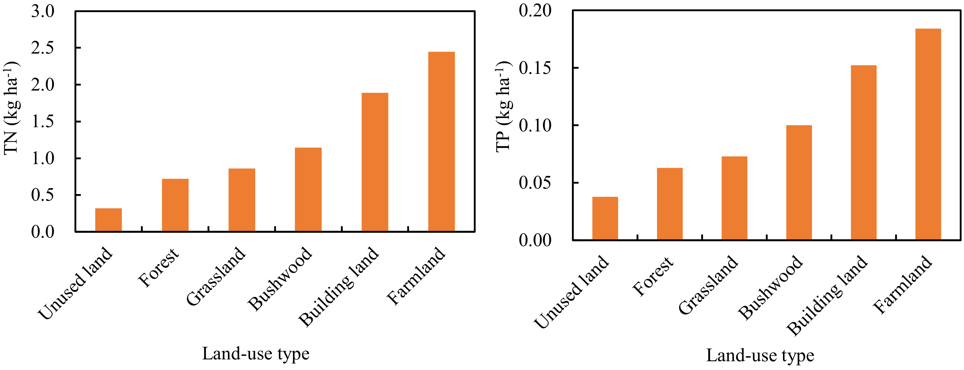
4.2.1. Land Use
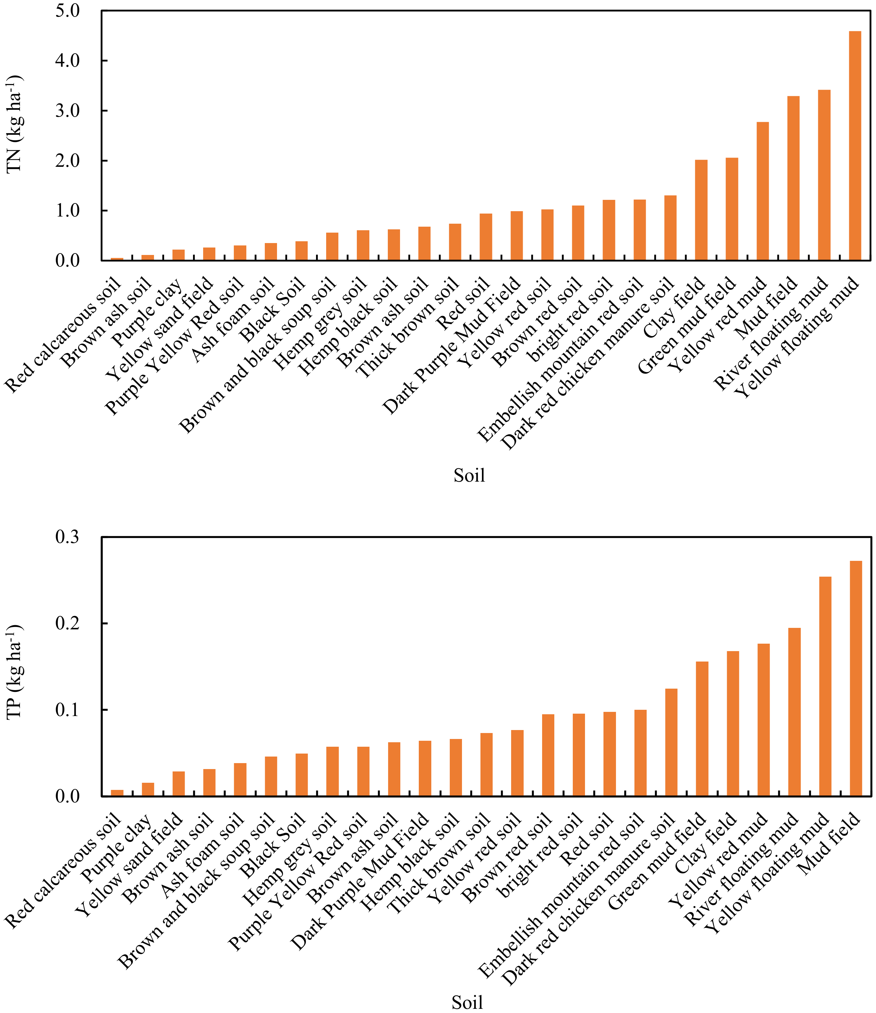
4.2.2. Soil
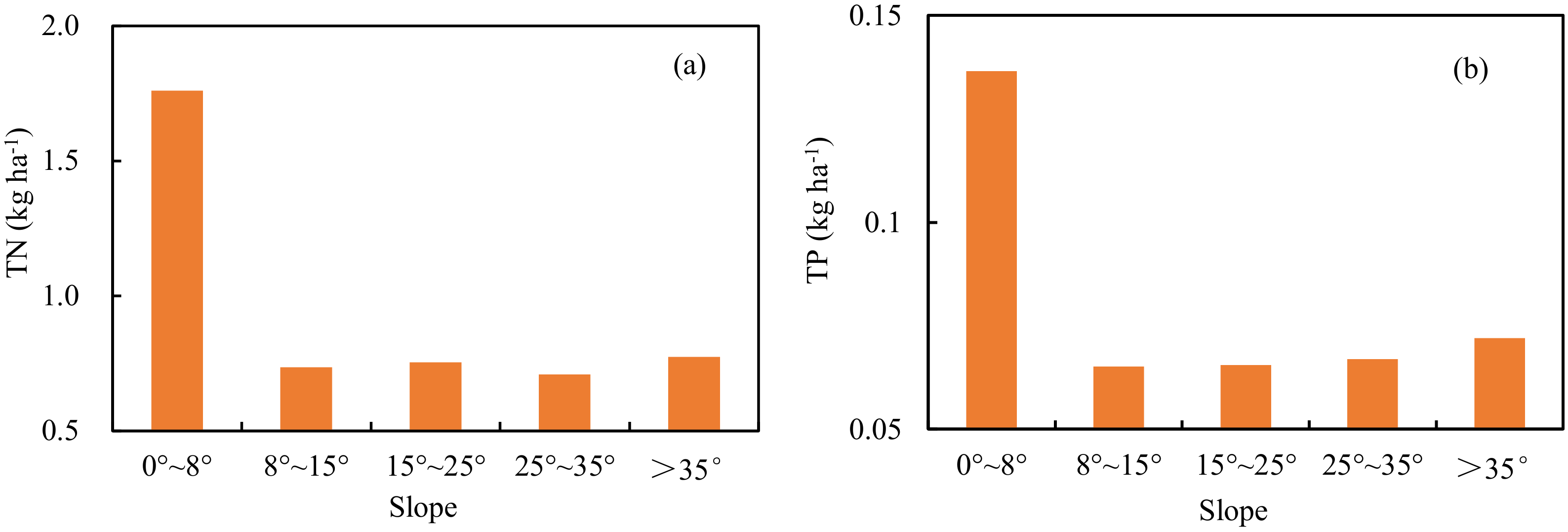
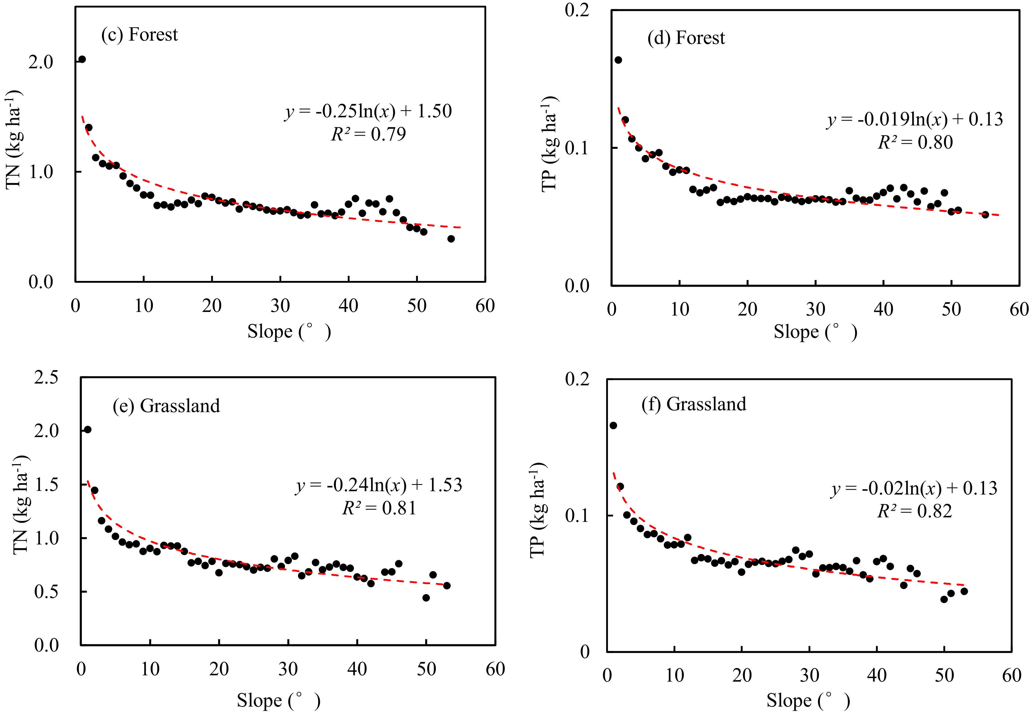
4.2.3. Slope
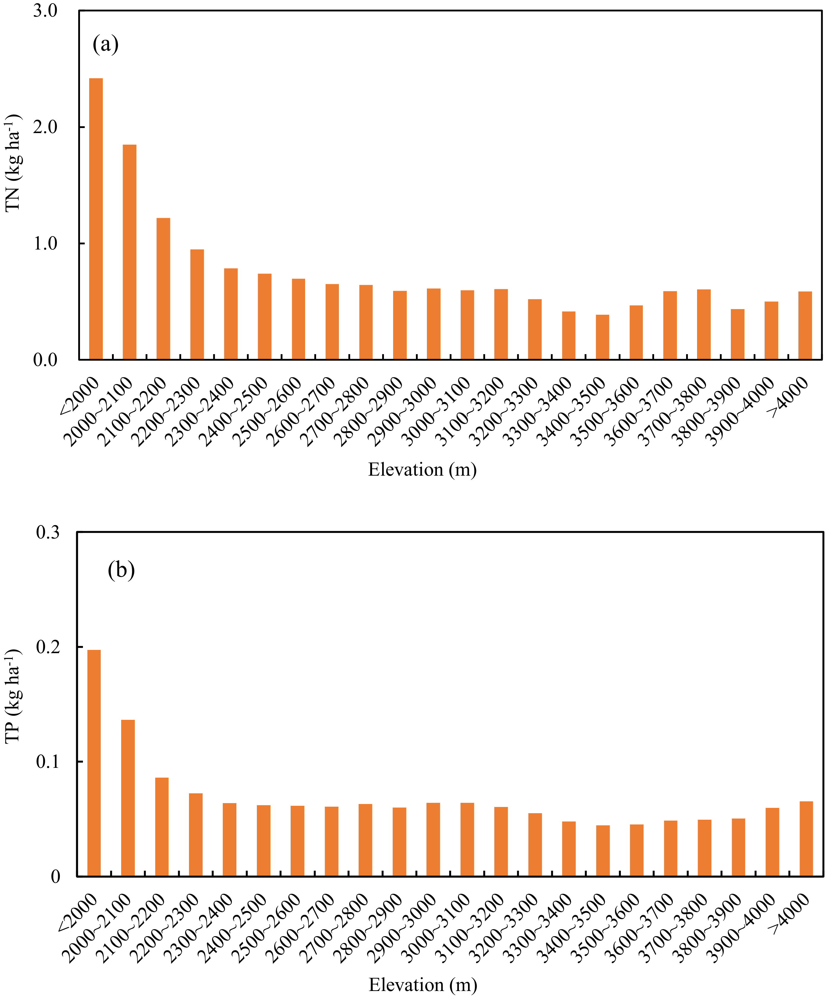
4.2.4. Elevation
5. Conclusions
- The pollution load intensity of farmland into the lake was the largest due to artificial fertilization and other reasons. Paddy soil exhibited the largest total nitrogen and total phosphorus pollution load.
- The pollution load intensity of agricultural land (dry land and paddy field) exhibited a quadratic functional relationship with the slope. The slope of 18° was a key topographic threshold for agricultural planting in the Erhai watershed. Therefore, in zones with slopes >18°, farming should be reduced as much as possible, and protective management measures such as terracing should be implemented.
- The load intensities contributed by the forest land and grassland showed logarithmic functional relationships with the slope. The load intensity declined with the increase in slope. Therefore, in steep regions, afforestation, returning farmland to forest, and other projects should be extensively promoted.
- The load intensities contributed from different land use types had logarithmic functional relationships with the geographical elevation. In the zones with geographical elevations smaller than 2000 m, the nitrogen and phosphorus pollution load intensities into the lake were relatively large, which were principally affected by the spatial distributions of farmland and residential construction land.
Author Contributions
Funding
Data Availability Statement
Conflicts of Interest
References
- Hou, C.; Librada, M.; Botero-Acosta, A.; Guzman, J.A. Modeling field scale nitrogen non-point source pollution (NPS) fate and transport: Influences from land management practices and climate. Sci. Total Environ. 2020, 759, 143502. [Google Scholar] [CrossRef] [PubMed]
- Ouyang, W.; Yang, W.; Tysklind, M.; Xu, Y.; Lin, C.; Gao, X.; Zhao, X. Using river sediments to analyze the driving force difference for non-point source pollution dynamics between two scales of watersheds. Water Res. 2018, 139, 311. [Google Scholar] [CrossRef] [PubMed]
- Chen, L.; Zhong, Y.; Wei, G.; Cai, Y.; Shen, Z. Development of an integrated modeling approach for identifying multilevel non-point-source priority management areas at the watershed scale. Water Resour. Res. 2014, 50, 4095–4109. [Google Scholar] [CrossRef]
- Han, D.; Currell, M.; Cao, G. Deep challenges for China’s war on water pollution. Environ. Pollut. 2016, 218, 1222–1233. [Google Scholar] [CrossRef] [PubMed]
- Srinivas, R.; Singh, A.; Dhadse, K.; Garg, C. An evidence based integrated watershed modelling system to assess the impact of non-point source pollution in the riverine ecosystem. J. Clean. Prod. 2020, 246, 118963. [Google Scholar] [CrossRef]
- Qian, Y.; Sun, L.; Chen, D.; Liao, J.; Sun, Q. The response of the migration of non-point source pollution to land use change in a typical small watershed in a semi-urbanized area. Sci. Total Environ. 2021, 785, 147387. [Google Scholar] [CrossRef]
- Zeng, J.; Huang, G.; Luo, H.; Mai, Y.; Wu, H. First flush of non-point source pollution and hydrological effects of LID in a Guangzhou community. Sci. Rep. 2019, 9, 13865. [Google Scholar] [CrossRef]
- Zhang, T.; Yang, Y.; Ni, J.; Xie, D. Construction of an integrated technology system for control agricultural non-point source pollution in the Three Gorges Reservoir Areas. Agric. Ecosyst. Environ. 2020, 295, 106919. [Google Scholar] [CrossRef]
- Chen, L.; Chen, S.; Li, S.; Shen, Z. Temporal and spatial scaling effects of parameter sensitivity in relation to non-point source pollution simulation. J. Hydrol. 2019, 571, 36–49. [Google Scholar] [CrossRef]
- Ouyang, W.; Hao, F.; Shi, Y.; Gao, X.; Gu, X.; Lian, Z. Predictive ability of climate change with the automated statistical downscaling method in a freeze-thaw agricultural area. Clim. Dyn. 2019, 52, 7013–7028. [Google Scholar] [CrossRef]
- Wan, W.; Han, Y.; Wu, H.; Liu, F.; Liu, Z. Application of the source–sink landscape method in the evaluation of agricultural non-point source pollution: First estimation of an orchard-dominated area in China. Agric. Water Manag. 2021, 252, 106910. [Google Scholar] [CrossRef]
- Xue, L.; Hou, P.; Zhang, Z.; Shen, M.; Yang, L. Application of systematic strategy for agricultural non-point source pollution control in Yangtze River basin, China. Agric. Ecosyst. Environ. 2020, 304, 107148. [Google Scholar] [CrossRef]
- Tao, Y.; Liu, J.; Guan, X.; Chen, H.; Ji, M. Estimation of potential agricultural non-point source pollution for Baiyangdian Basin, China, under different environment protection policies. PLoS ONE 2020, 15, e0239006. [Google Scholar] [CrossRef] [PubMed]
- Luo, X.; Wu, W.; He, D.; Li, Y.; Ji, X. Hydrological Simulation Using TRMM and CHIRPS Precipitation Estimates in the Lower Lancang-Mekong River Basin. Chin. Geogr. Sci. 2019, 29, 13–25. [Google Scholar] [CrossRef]
- Chen, X.; Liu, X.; Peng, W.; Dong, F.; Huang, Z.; Wang, R. Non-Point Source Nitrogen and Phosphorus Assessment and Management Plan with an Improved Method in Data-Poor Regions. Water 2017, 10, 17. [Google Scholar] [CrossRef]
- Maringanti, C.; Chaubey, I.; Arabi, M.; Engel, B. Application of a multi-objective optimization method to provide least cost alternatives for NPS pollution control. Environ. Manag. 2011, 48, 448–461. [Google Scholar] [CrossRef]
- Nilawar, A.; Waikar, M. Impacts of climate change on streamflow and sediment concentration under RCP 4.5 and 8.5: A case study in Purna river basin, India. Sci. Total Environ. 2019, 650, 2685–2696. [Google Scholar] [CrossRef]
- Daniel, B.; Tena, A.; Asfaw, K.; Gete, Z.; Assefa, M. Modeling Climate Change Impact on the Hydrology of Keleta Watershed in the Awash River Basin, Ethiopia. Environ. Modeling Assess. 2018, 24, 1–13. [Google Scholar]
- Wen, X.; Liu, Z.; Lei, X.; Lin, R.; Fang, G.; Tan, Q.; Wang, C.; Tian, Y.; Quan, J. Future changes in Yuan River ecohydrology: Individual and cumulative impacts of climates change and cascade hydropower development on runoff and aquatic habitat quality. Sci. Total Environ. 2018, 633, 1403. [Google Scholar] [CrossRef]
- Peraza-Castro, M.; Ruiz-Romera, E.; Meaurio, M.; Sauvage, S.; Sánchez-Pérez, J. Modelling the impact of climate and land cover change on hydrology and water quality in a forest watershed in the Basque Country (Northern Spain). Ecol. Eng. 2018, 122, 315–326. [Google Scholar] [CrossRef]
- Rui, Y.; Zhang, X.; Yan, S.; Zhang, J.; Hao, C. Spatial patterns of hydrological responses to land use/cover change in a catchment on the Loess Plateau, China. Ecol. Indic. 2018, 92, 151–160. [Google Scholar]
- Hyandye, C.; Worqul, A.; Martz, L.; Muzuka, A. The impact of future climate and land use/cover change on water resources in the Ndembera watershed and their mitigation and adaptation strategies. Environ. Syst. Res. 2018, 7, 7. [Google Scholar] [CrossRef]
- Kaandorp, V.; Molina-Navarro, E.; Andersen, H.; Bloomfield, J.; Kuijper, M.; Louw, P. A conceptual model for the analysis of multi-stressors in linked groundwater–surface water systems. Sci. Total Environ. 2018, 627, 880–895. [Google Scholar] [CrossRef] [PubMed]
- Hoang, L.; Schneiderman, E.; Moore, K.; Mukundan, R.; Owens, E.; Steenhuis, T. Predicting saturation-excess runoff distribution with a lumped hillslope model: SWAT-HS. Hydrol. Process. 2017, 31, 2226–2243. [Google Scholar] [CrossRef]
- Hu, S.; Yang, D.; Wu, J.; Gao, Y.; Qiu, H.; Cao, M.; Song, J.; Wan, H. Spatio-temporal Variation Characteristics of Baseflow in the Bahe River Basin Based on Digital Filter Method and SWAT Model. Sci. Geogr. Sin. 2017, 37, 455–463. [Google Scholar]
- Foteh, R.; Garg, V.; Nikam, B.; Khadatare, M.; Aggarwal, S.; Kumar, A. Reservoir Sedimentation Assessment through Remote Sensing and Hydrological Modelling. J. Indian Soc. Remote Sens. 2018, 46, 1893–1905. [Google Scholar] [CrossRef]
- Mohammad, H.; Assefa, M.; Hector, F. Erosion and Sediment Transport Modelling in Shallow Waters: A Review on Approaches, Models and Applications. Int. J. Environ. Res. Public Health 2018, 15, 518. [Google Scholar]
- Le Roux, J. Sediment Yield Potential in South Africa’s Only Large River Network without a Dam: Implications for Water Resource Management: Sediment Yield in South Africa’s Only Large River without a Dam. Land Degrad. Dev. 2018, 29, 765–775. [Google Scholar] [CrossRef]
- Zeiger, S.; Hubbart, J. A SWAT model validation of nested-scale contemporaneous stream flow, suspended sediment and nutrients from a multiple-land-use watershed of the central USA. Sci. Total Environ. 2016, 572, 232–243. [Google Scholar] [CrossRef]
- Özcan, Z.; Kentel, E.; Alp, E. Determination of unit nutrient loads for different land uses in wet periods through modelling and optimization for a semi-arid region. J. Hydrol. 2016, 540, 40–49. [Google Scholar] [CrossRef]
- Alemayehu, T.; Griensven, A.; Woldegiorgis, B.; Bauwens, W. An improved SWAT vegetation growth module and its evaluation for four tropical ecosystems. Hydrol. Earth Syst. Sci. 2017, 21, 4449–4467. [Google Scholar] [CrossRef]
- Zhao, F.; Wu, Y.; Qiu, L.; Sivakumar, B.; Zhang, F.; Sun, Y. Spatio-temporal features of the hydro-biogeochemical cycles in a typical loess gully watershed. Ecol. Indic. 2018, 91, 542–554. [Google Scholar] [CrossRef]
- Evenson, G.; Golden, H.; Lane, C.; Mclaughlin, D.; D’Amico, E. Depressional Wetlands Affect Watershed Hydrological, Biogeochemical, and Ecological Functions. Ecol. Appl. 2018, 28, 953–966. [Google Scholar] [CrossRef]
- Ni, X.; Parajuli, P. Evaluation of the impacts of BMPs and tailwater recovery system on surface and groundwater using satellite imagery and SWAT reservoir function. Agric. Water Manag. 2018, 210, 78–87. [Google Scholar] [CrossRef]
- Imani, S.; Niksokhan, M.; Jamshidi, S.; Abbaspour, K. Discharge permit market and farm management nexus: An approach for eutrophication control in small basins with low-income farmers. Environ. Monit. Assess. 2017, 189, 346. [Google Scholar] [CrossRef] [PubMed]
- Ouyang, W.; Hao, F.; Wang, X.; Cheng, H. Nonpoint Source Pollution Responses Simulation for Conversion Cropland to Forest in Mountains by SWAT in China. Environ. Manag. 2008, 41, 79–89. [Google Scholar] [CrossRef] [PubMed]
- Shen, Z.; Chen, L.; Hong, Q.; Qiu, J.; Xie, H.; Liu, R. Assessment of nitrogen and phosphorus loads and causal factors from different land use and soil types in the Three Gorges Reservoir Area. Sci. Total Environ. 2013, 454–455, 383–392. [Google Scholar] [CrossRef]
- Shen, Z.; Chen, L.; Hong, Q.; Xie, H.; Qiu, J.; Liu, R. Vertical Variation of Nonpoint Source Pollutants in the Three Gorges Reservoir Region. PLoS ONE 2013, 8, e71194. [Google Scholar] [CrossRef][Green Version]
- Ge, Y.; Xue, B.; Lai, G.; Feng, G.; Liu, X. A 200-year historical modeling of catchment nutrient changes in Taihu basin, China. Hydrobiologia 2007, 581, 79–87. [Google Scholar]
- Kenea, U.; Adeba, D.; Regasa, M.S.; Nones, M. Hydrological Responses to Land Use Land Cover Changes in the Fincha’a Watershed, Ethiopia. Land 2021, 10, 916. [Google Scholar] [CrossRef]
- Cibin, R.; Sudheer, K.; Chaubey, I. Sensitivity and identifiability of stream flow generation parameters of the SWAT model. Hydrol. Process. 2010, 24, 1133–1148. [Google Scholar] [CrossRef]
- Herman, J.; Kollat, J.; Reed, P.; Wagener, T. Technical Note: Method of Morris effectively reduces the computational demands of global sensitivity analysis for distributed watershed models. Hydrol. Earth Syst. Sci. 2013, 17, 2893–2903. [Google Scholar] [CrossRef]
- Guse, B.; Pfannerstill, M.; Kiesel, J.; Strauch, M.; Fohrer, N. Analysing spatio-temporal process and parameter dynamics in models to characterise contrasting catchments. J. Hydrol. 2019, 570, 863–874. [Google Scholar] [CrossRef]
- Chen, Y.; Marek, G.; Marek, T.; Porter, D.; Srinivasan, R. Simulating the effects of agricultural production practices on water conservation and crop yields using an improved SWAT model in the Texas High Plains, USA. Agric. Water Manag. 2021, 244, 106574. [Google Scholar] [CrossRef]
- Cheng, Y.; Ao, T.; Li, X.; Wu, B. Runoff simulation by SWAT model based on parameters transfer method in ungauged catchments of middle reaches of Jialing River. Trans. Chin. Soc. Agric. Eng. 2016, 32, 81–86. [Google Scholar]
- Wu, B.; Li, X.; Ao, T.; Fan, Y.; Wang, X. Study of SWAT Model Based on Parameter Transfer Method in Data Scarce Catchment for Non-point Source Pollution Simulation. J. Sichuan Univ. (Eng. Sci. Ed.) 2015, 47, 9–16. [Google Scholar]
- Hong, Q.; Sun, Z.; Chen, L.; Liu, R.; Shen, Z. Small-scale watershed extended method for non-point source pollution estimation in part of the Three Gorges Reservoir Region. Int. J. Environ. Sci. Technol. 2012, 9, 595–604. [Google Scholar] [CrossRef]
- Shang, X.; Wang, X.; Zhang, D.; Chen, W.; Chen, X.; Kong, H. An improved SWAT-based computational framework for identifying critical source areas for agricultural pollution at the lake basin scale. Ecol. Model. 2012, 226, 1–10. [Google Scholar] [CrossRef]
- Wang, S. Eutrophication Process and Mechanism of Erhai Lake; Science Press: Beijing, China, 2015. [Google Scholar]
- Li, Y.; Wang, C.; Tang, H. Research advances in nutrient runoff on sloping land in watersheds. Aquat. Ecosyst. Health Manag. 2006, 9, 27–32. [Google Scholar] [CrossRef]
- Yang, G.; Best, E.; Whiteaker, T.; Teklitz, A.; Yeghiazarian, L. A screening-level modeling approach to estimate nitrogen loading and standard exceedance risk, with application to the Tippecanoe River watershed, Indiana. J. Environ. Manag. 2014, 135, 1–10. [Google Scholar] [CrossRef] [PubMed]
- Li, Y.; Li, B.; Zhang, K.; Zhu, J.; Yang, Q. Study on spatiotemporal distribution characteristics of annual precipitation of Erhai Basin. J. China Inst. Water Resour. Hydropower Res. 2017, 15, 234–240. [Google Scholar]
- McGrath, S.; Zhao, X.; Steele, R.; Thombs, B.; Benedetti, A.; DEPRESSED Collaboration. Estimating the sample mean and standard deviation from commonly reported quantiles in meta-analysis. Stat. Methods Med. Res. 2020, 29, 2520–2537. [Google Scholar] [CrossRef] [PubMed]
- Dahri, N.; Abida, H. Monte Carlo simulation-aided analytical hierarchy process (AHP) for flood susceptibility mapping in Gabes Basin (southeastern Tunisia). Environ. Earth Sci. 2017, 76, 302. [Google Scholar] [CrossRef]


| Data Type | Scale | Source | Data Description |
|---|---|---|---|
| Elevation | 1:250,000 | Geospatial Data Cloud. Available online: http://www.gscloud.cn (accessed on 13 November 2021) | Sub-watershed division basis, geographic elevation, slope, slope length in 2015 |
| Soil type | 1:1,000,000 | Institute of Soil Science, Chinese Academy of Sciences | Classification of soil types and physicochemical properties of soil in 2010 |
| Land use type | 1:100,000 | Remote sensing image interpretation | Classification of land use types in 2016 |
| Meteorological | 13 stations | China Meteorological Data Network (http://data.cma.cn, accessed on 13 November 2021) | Precipitation, temperature, evaporation, wind speed, relative humidity, solar radiation from 2013 to 2017 |
| Hydrology and water quality | Dali Branch of Yunnan Hydrology and Water Resources Bureau | Physical and chemical indexes such as river discharge, nitrogen and phosphorus from 2013 to 2017 | |
| Socioeconomic data | Dali Prefecture Agriculture Bureau | Crop planting type, planting and harvest time. Fertilization type, time and amount from 2013 to 2017 | |
| Water conservancy project | Three medium-sized reservoirs | Dali Branch of Yunnan Hydrology and Water Resources Bureau | Reservoir capacity, operating water level, inbound and outbound flow, and water quality from 2013 to 2017 |
| Zone | Average Precipitation/mm | Average Elevation/m | Average Slope/° | Average Vegetation Coverage |
|---|---|---|---|---|
| North | 790.7 | 2631.0 | 13.89 | 0.34 |
| West | 1097.1 | 2587.4 | 18.95 | 0.48 |
| South | 804.5 | 2283.2 | 12.95 | 0.38 |
| East | 773.5 | 2225.2 | 11.88 | 0.24 |
| Variable | North | West | South | East | ||||
|---|---|---|---|---|---|---|---|---|
| Parameter | Rank | Parameter | Rank | Parameter | Rank | Parameter | Rank | |
| Flow | CN2.mgt | 1 | ALPHA_BF.gw | 1 | ALPHA_BF.gw | 1 | CN2.mgt | 1 |
| ALPHA_BF.gw | 2 | SLSUBBSN.hru | 2 | CN2.mgt | 2 | SOL_AWC.sol | 2 | |
| SURLAG.bsn | 3 | CH_N2.rte | 3 | CH_K2.rte | 3 | SOL_K.sol | 3 | |
| GW_REVAP.gw | 4 | CN2.mgt | 4 | SLSUBBSN.hru | 4 | ALPHA_BF.gw | 4 | |
| CH_N2.rte | 5 | SOL_AWC.sol | 5 | SOL_AWC.sol | 5 | ESCO.hru | 5 | |
| P | SOL_ORGP.chm | 1 | SOL_ORGP.chm | 1 | SOL_ORGP.chm | 1 | SOL_ORGP.chm | 1 |
| SOL_SOLP.chm | 2 | SOL_SOLP.chm | 2 | SOL_SOLP.chm | 2 | SOL_SOLP.chm | 2 | |
| PPERCO.bsn | 3 | PPERCO.bsn | 3 | PPERCO.bsn | 3 | PPERCO.bsn | 3 | |
| N | CDN.bsn | 1 | CDN.bsn | 1 | SOL_ORGN.chm | 1 | SOL_OGRN.chm | 1 |
| SDNCO.bsn | 2 | SDNCO.bsn | 2 | CDN.bsn | 2 | SOL_NO3.chm | 2 | |
| SOL_OGRN.chm | 3 | SOL_OGRN.chm | 3 | SDNCO.bsn | 3 | NPERCP.bsn | 3 | |
| River | Variable | Calibration | Validation | ||
|---|---|---|---|---|---|
| R2 | Ens | R2 | Ens | ||
| MJ | Flow | 0.92 | 0.91 | 0.88 | 0.85 |
| NH3-N | 0.77 | 0.71 | 0.73 | 0.72 | |
| TP | 0.89 | 0.80 | 0.88 | 0.71 | |
| YX | Flow | 0.94 | 0.91 | 0.88 | 0.84 |
| TN | 0.86 | 0.78 | 0.74 | 0.71 | |
| TP | 0.82 | 0.80 | 0.79 | 0.79 | |
| BS | Flow | 0.90 | 0.85 | 0.86 | 0.81 |
| TN | 0.83 | 0.81 | 0.79 | 0.76 | |
| TP | 0.81 | 0.78 | 0.83 | 0.76 | |
| MC | Flow | 0.92 | 0.90 | 0.88 | 0.83 |
| TN | 0.86 | 0.75 | 0.87 | 0.78 | |
| TP | 0.85 | 0.78 | 0.91 | 0.81 | |
| BL | Flow | 0.94 | 0.93 | 0.83 | 0.83 |
| TN | 0.85 | 0.85 | 0.88 | 0.81 | |
| TP | 0.92 | 0.87 | 0.88 | 0.84 | |
| YL | Flow | 0.74 | 0.70 | 0.70 | 0.63 |
| TN | 0.88 | 0.62 | 0.83 | 0.58 | |
| TP | 0.66 | 0.63 | 0.59 | 0.53 | |
Publisher’s Note: MDPI stays neutral with regard to jurisdictional claims in published maps and institutional affiliations. |
© 2021 by the authors. Licensee MDPI, Basel, Switzerland. This article is an open access article distributed under the terms and conditions of the Creative Commons Attribution (CC BY) license (https://creativecommons.org/licenses/by/4.0/).
Share and Cite
Chen, X.; He, G.; Liu, X.; Li, B.; Peng, W.; Dong, F.; Huang, A.; Wang, W.; Lian, Q. Sub-Watershed Parameter Transplantation Method for Non-Point Source Pollution Estimation in Complex Underlying Surface Environment. Land 2021, 10, 1387. https://doi.org/10.3390/land10121387
Chen X, He G, Liu X, Li B, Peng W, Dong F, Huang A, Wang W, Lian Q. Sub-Watershed Parameter Transplantation Method for Non-Point Source Pollution Estimation in Complex Underlying Surface Environment. Land. 2021; 10(12):1387. https://doi.org/10.3390/land10121387
Chicago/Turabian StyleChen, Xuekai, Guojian He, Xiaobo Liu, Bogen Li, Wenqi Peng, Fei Dong, Aiping Huang, Weijie Wang, and Qiuyue Lian. 2021. "Sub-Watershed Parameter Transplantation Method for Non-Point Source Pollution Estimation in Complex Underlying Surface Environment" Land 10, no. 12: 1387. https://doi.org/10.3390/land10121387
APA StyleChen, X., He, G., Liu, X., Li, B., Peng, W., Dong, F., Huang, A., Wang, W., & Lian, Q. (2021). Sub-Watershed Parameter Transplantation Method for Non-Point Source Pollution Estimation in Complex Underlying Surface Environment. Land, 10(12), 1387. https://doi.org/10.3390/land10121387