Resource Opportunity in China’s Market Transition and Governance: Time Factor in Urban Housing Inequality

Abstract

Since China’s reform and opening up, the country’s rapid marketization process has been accompanied by the rapid growth of inequality, which has been significant for all classes of society. In terms of its impact, housing inequality is particularly noticeable. In this paper, we discuss the influence of real-estate purchase time, organization, human capital, and political capital on the value of real estate and the appreciation of real estate in China by using a conditional mean model and a quantile regression model. The differences in the degree of influence of these factors on different quantile levels are also investigated. We found that, after adding the time factor, the prior possession of resources in the early stage of market transformation will benefit the long-term marketization process. Organizations that can penetrate “market-redistribution” and professions that directly participate in the distribution of real-estate resources also have significant advantages in this regard.

1. Introduction

Since China’s reform and opening up in 1978, the country’s high-speed process of marketization has resulted in unprecedented advancements. Additionally, concerns, such as imbalanced and insufficient developments, ensued, with social inequality becoming the most serious issue. In the early 1980s, China and other Eastern European socialist countries were the most equal countries in the world. Then, the Gini coefficient in China was less than 0.3, which was lower than that of developed countries and other developing countries [1]. Despite official statistics indicating a drop in the Gini coefficient in China during these years—0.49 in 2008 to 0.46 in 2015 [2]—the nation has undeniably transformed from one of the most equal countries in the world into one of the world’s most unequal countries over the last 40 years. This transition has exerted a profound influence on every stratum of society, and housing inequality is the most remarkable problem.

Several issues account for this phenomenon of inequality, one of which is the commodification of housing. The homeownership rate of Chinese urban residents increased from 15% in 1995 to 80% in 2002, and the latter number was even higher than the figure for the United States in 2003, which was 68% [3,4]. Thus, a real-estate market emerged from the old system of socialist redistribution.

Residents have gone from a period marked by “houses allocated by work units” to a period characterized by “buying houses on their own” within a generation. The old institutional arrangements and the force of marketization are intertwined, forming a medley of houses with different historical origins on the market. Additionally, the housing allocation circumstances of society and the complex arrangements in economics and society are intertwined, resulting in housing inequality.

Notably, housing prices are rapidly increasing, and two aspects account for this trend. First, many people in China leave their hometowns to seek employment in big cities. As a result, there is considerable demand for housing in these cities. Second, under circumstances marked by inflation and a sluggish manufacturing industry, housing hash has become the fastest-growing value-added asset of Chinese families. The average profitability rates of first-, second-, and third-owned urban residences are 340.31%, 143.25%, and 96.70%, respectively [5]. Therefore, housing inequality is more than a matter of social resource distribution, such as income inequality. The accompanying high profitability is more likely to become an institutionalized source of rent-seeking. Individuals who invest early tend to receive a substantial amount of added value through real-estate appreciation and residential rental properties, creating even wider inequality. This will probably lead to a more rigorous problem—the Matthew Effect. The Matthew Effect means that any individual, group, or region that achieves success and progress in a certain aspect (such as money, reputation, status, etc.) will produce an accumulated advantage and have more opportunities to achieve greater success and progress [6]. What are the characteristics of housing inequality? Which stratum of society owns high-value properties? Who can benefit from the property market? All of these questions must be studied and solved in greater detail.

2. Theory and Hypothesis

Since the 1980s, the relation between China’s market transition and social stratification has been a main focus in academic research, and scholars have performed productive research in this respect. Although judgments vary regarding social inequality in early socialist China, many scholars have emphasized that the redistribution of collective goods is likely to form greater inequality than once thought against the background of “egalitarianism” in a redistribution structure bonded by a unit system [7,8,9,10]. Correspondingly, such a habit of redistribution of collective goods is likely to continue even after market transition due to institutional inertia or path dependence [11,12].

Housing is a clear example of this. In the early days of the reform, many urban residents could purchase houses at a price lower than the market price through their work unit ties or social relations [10,13,14]. In recent years, many empirical studies have indicated a gradual widening of housing inequality in urban residents from every stratum of society [15,16]. From the perspective of market transition theory [17,18], housing inequality among different strata is inevitable and will decline because the market transition will form a new means of resource allocation under a redistribution system. In this emerging market, the influence of old political capital declines, and market mechanisms focused more on individual capabilities and fair competition assume greater importance. Because of the Matthew Effect from competition, housing inequality will widen in the short-term. In the process, the return on human capital, such as education, will increase, and the return on political capital, such as party membership and cadre position, will decrease. Compared with old powerful elites, current market elites have gained new access to real-estate profits. Market transition will eventually create a fairer and more equal housing supply mechanism. With the further deepening of the market transition, ever more people with substantial human capital are able to profit from it, and inequality will eventually decline due to the more thorough social security system established by the government [19].

Another theory is the Power Continuance Theory or the Power Transition Theory [20], which underscores that the state’s power creates an innate advantage and a stronger ability to expand in the process of market transition. Additionally, compared with other governments, local governments in China tend to participate in economic construction more actively under the pressure of political achievement in terms of economic development [21]. These factors justify the further expansion of bureaucracy in the market, and government functions also become stronger. Under such circumstances, factors such as political capital may assume greater importance in the process of market transition. Empirical studies have also demonstrated the positive effect of the work unit system and public power on property area and purchasing opportunity [22]. Additionally, income studies have shown that China ranks relatively low among developing countries regarding the monetary return on one extra year of schooling. Additionally, the income advantage of Chinese Communist Party membership is remarkable [23]. Chinese Communist Party membership is often regarded as a kind of political capital [24], similar to a kind of social capital (relationship), which can obtain many resources (information, influence, or operation power) and opportunities [25]. In other words, party members have the opportunity to contact people who are highly beneficial to their future careers [26]. The aforementioned statistics support the argument of power continuance.

The major difference between market transition theory and power continuance theory is that the resources brought by market reform are acquired by new market elites or old powerful elites. The common assumption of the two theories is as follows: China’s marketization reform cannot be achieved instantly; by contrast, it continues gradually. The marketization level of China seems to increase continuously and is now in its preliminary stage. Marketization is bound to offer a dynamic aspect to economic development. The advantage of such an assumption is that the stimulating effect of the market on economic development has been clearly expounded in economics [27]. Needless to say, the market improves the efficiency of the economy in a broader sense. Although market transition advances step by step, means of production, such as commodity, workforce, and property, slowly form their respective markets simultaneously. However, these markets almost complete the commodification process overnight, which is characterized by “punctuated” institutional changes (Punctuated-Equilibrium Theory, for reference). The time factor has tended to be ignored in the literature. Based on CHIP long-term statistics, Li concluded that the pronounced wealth inequality of Chinese residents began between 1995 and 2002 [28].

Additionally, based on mean regression studies [29,30], one problem that can easily be ignored in many cases is that unequal models vary among different groups of people. The progressive reform functioning as “China’s experience” is the fundamental logic of Chinese urban residence institutional reform and avoids overall turbulence in the reform process. Notably, something else ensues; because the basic attribute of urban residence and the concept of equality of urban residents have been changed, the difference in housing benefits acquired by individuals from every stratum of society has accumulated and strengthened, and this allows the market capability of residents to play a bigger role in social stratification [31]. Due to the ongoing process of marketization and social stratification, housing will continue to strengthen the benefits of individuals who already own a house. Additionally, people in a relatively low-income class will find profiting from the property market more difficult. Another technical problem is that plenty of papers on housing inequality have been published based on survey data from around 2005 [32,33]. Additionally, the independent variable has tended to be living space; thus, property value has not been fully studied. As such, there is a gap in the literature that is worthwhile filling.

To sum up, some classic hypotheses and propositions in previous theories can be borrowed to illustrate housing inequality:

Hypothesis 1a.

The higher the educational level, the higher the housing value.

Hypothesis 1b.

The higher the income, the higher the housing value.

Hypothesis 2a.

The cadre position has a greater advantage than other occupations in terms of housing value.

Hypothesis 2b.

People with party membership have a greater advantage than non-party people in terms of housing allocation and acquirement.

Hypothesis 3a.

It is easier for non-market organizations, such as state-owned enterprises and the party and government organs, to acquire high-value housing than market units in a manner similar to private enterprises and self-employed individuals.

Hypothesis 3b.

Non-market organizations, such as state-owned enterprises and the party and government organs, profit more from the property market than market units, such as private enterprises and self-employed individuals.

This paper proposes the following research hypotheses:

Hypothesis 4a.

Time factor. Against the backdrop of progressive reform, individuals who enter the property market late receive relatively high returns due to fully developed marketization.

Hypothesis 4b.

Time factor. Against the backdrop of progressive reform, individuals who enter the real-estate market late receive relatively low returns due to a limited holding period for housing.

Above all, a close and hierarchical analysis is conducted for people receiving different levels of housing profits.

3. Research Methods

3.1. Methodology

Regarding research methodology, this paper adopts a quantile regression model and the common ordinary least squares (OLS) linear regression model found in the literature. Compared with an OLS linear regression model based on mean, a quantile regression model has two advantages. First, the quantile is less likely to be affected by extreme values than the mean. Although such a problem can be alleviated by taking logarithms of variables in the mean regression, quantile regression is better in terms of managing skewed variables, such as income and housing value. Second, regression equations can be established according to different quantile levels of dependent variables. Therefore, all factors can be closely studied under the influence of all sorts of housing profitability levels. Furthermore, the changing patterns of these factors in different quantile levels can be analyzed, which is better than the over-general conclusion reached under the guidance of the OLS model.

This paper adopts 19 quantiles from 5 to 95 at an interval of 5; additionally, it selects a multivariable linear regression model, in which every dependent variable has 20 regression equations. Thus, an analysis based on regression excels can be conducted as performed in classic quantitative research. Additionally, regression coefficient tables in different quantiles can be created to inspect the changing patterns of independent variables in different quantile levels.

3.2. Data Collection

This paper adopts data from the Social Development and Social Construction national survey conducted by Shanghai University in 2012. The survey applies simple random sampling in three stages, and the data are from various geographical locations in China, namely Henan Province, Jilin Province, the municipality of Shanghai, Guangdong Province, Yunnan Province, and Gansu Province. The total number of samples is 5745. Due to the substantial differences between a rural homestead self-built house system and a commoditized urban property market, 2482 rural samples were excluded from this research. Among the remaining samples, 2041 people either purchased or built houses on their own. These people in question claimed the right to their property, know the price of their property, and are the main research objects in this paper.

3.3. Measures

Dependent variable 1 is the total value of the main residence. Because the property market in China is relatively mature, the housing price of the respondents includes information about housing quality and housing location, which is a suitable variable to represent the distribution of housing resources. Dependent variable 2 is the added value of the house after purchase or construction. Because respondents are asked on the questionnaires to provide the date when they purchased or built their house and the cost of doing so, the added value of the house in question can be calculated from the date of the contract to the year 2012, when the survey was conducted. This variable indicates the profit of respondents from the property market and allows us to more accurately operationalize incremental resources in the process of market transition. Logarithms have been taken of the two variables in the OLS model because the two variables are skewed to the right. Although it is necessary to take logarithms in the quantile model, natural logarithms of dependent variables have been used improve the comparison of the results of the OLS model. The main independent variables are as follows:

• Education level: The education of the respondents is re-classified as elementary school and below, secondary school, high school, and university and above.
• Party membership: Membership includes Communist Party membership and membership in democratic parties. In China, democratic parties have their own political implications.
• Work unit type: Due to the joint-stock system reform in recent years, some state-owned enterprises and collective enterprises have begun to include private capital, and some public institutions are owned and run by individuals. Therefore, first, the work unit types offered in questionnaires are roughly classified. Next, the work unit types marked as enterprise are further classified as state-owned, collective, or privately owned in terms of ownership.
• Occupation and administration position: Occupation is a major factor affecting housing distribution. To better compare the variable of administration position to other occupations, respondents with an administration position are encoded into two professions: senior cadres with a title of section chief and above, and junior cadres with a title of section chief and below. These two professions are added to the variable of occupation. Additionally, samples that have both administration positions and other occupations are ruled out.
• Control variable: According to the literature, demographic variables are included as control variables to increase the accuracy of the model. These variables are age and the square of age, marital status, number of family members, province, and natural logarithm, taken as the total income of the previous year.

Another independent variable warranting attention in this paper is the time when the house was purchased or built. Although this independent variable is a continuous variable on the questionnaire, this paper de-dimensionalizes it into four nominal variables: before 1998, 1999–2003, 2004–2008, and 2009–2012. The years 1998, 2003, and 2008 are selected as key division points due to theoretical and historical reasons. According to the research conducted by Wu Xiaobo [34], the then incumbent Zhu Rongji administration suspended the policy of selling state capital to private businesses, which targeted the state-owned small and medium enterprises with poor performance. After 1998, state-owned capital withdrew from competitive industries, such as textiles, home appliances, and food, while playing a dominant and monopolistic role in strategic industries, such as resources, energy, and heavy chemicals. State-owned businesses started to retreat to the upper-stream industries, forming an advantage of an oligarchy or multi-oligarchy operation.

After 1998, the housing of urban residents transformed from work–unit-distributed houses into commodity houses for transactional purposes. At the end of 2003, the State Council released Provisions on Curbing Blind Investment in Steel, Electrolytic Aluminum, Cement and other industries, to manage the over-popular investments in energy industries. Additionally, in 2003, the State-Owned Assets Supervision and Administration Commission of the State Council was founded. In the following three years, the main business income of enterprises directly under central authorities increased by 78.8%, the profit increased by 140%, the tax revenue increased by 96.5%, and the hedge ratio of state-owned assets increased to 144.4%. Feng Lun, then chairman of Wangtong Group, said, “Faced with state-owned capital, private capital has to stick to the principle of cooperation over competition, supplement over substitution, affiliation over dominance. Only by accomplishing this can the private capital advance continuously and fare well”.

In 2008, because exports were hindered by the financial crisis, the central government implemented a proactive fiscal policy—a USD 4 trillion economy stimulus package. As a result, state-owned enterprises gained 90% of the new loans. Above all, 1998 was the starting point of the commodification of housing, and 2003 and 2008 were significant years because the administration increased the investment in state-owned capital and private capital withdrew from the production field during the process of market transition. Furthermore, the private capital withdrawn in 2003 and 2008 was mostly transferred to the financial market, in which the real-estate market, as the fastest-growing value-added investment, received substantial attention. In the process of property investment, local governments also profited from land finance, namely collecting land transaction fees by transferring land use rights [35]. Additionally, state-owned enterprises can profit from the upstream industries resulting from property construction. A prohibitive housing price scenario is the result of the common interests of private capital, local governments, and state-owned capital. Therefore, the years 1998, 2003, and 2008 are particularly important because they have different implications for housing prices. The time when the property market was entered is divided into four stages.

The descriptive statistics of the aforementioned variables are in

Table 1. Descriptive statistics of variables.

Continuous Variable
Variables	Sample Numbers	Mean	Gini Coefficient	Standard Deviation	Minimum Value	Maximum Value
The market value of property 1 (CNY 10,000)	2791	80.67	0.59332	128.46	0.01	3000
The added value of property (CNY 10,000)	1931	55.88	0.57414	70.977	−49	990
Income (CNY)	3165	44,700	0.58174	534,295	300	3 × 107
Number of properties	2860	1.203	——	0.5986	1	15
Year of purchase or construction	1998	2000	——	9.6015	1812	2013
Age	3263	42.54	——	14.224	17	70
Discrete variable 2
Variables	Sample numbers	Frequency	Percentage (%)	Standard deviation	Minimum value	Maximum value
Time of Purchase or Construction
Before 1998	1998	659	32.983	0.4703	0	1
1999–2003	1998	555	27.7778	0.448	0	1
2004–2008	1998	479	23.974	0.427	0	1
After 2009	1998	305	15.2653	0.3597	0	1
Work Unit Types
Party and government organs	2891	94	3.25147	0.1774	0	1
Public institutions	2891	426	14.7354	0.3545	0	1
State-owned enterprises	2891	669	23.1408	0.4218	0	1
Collective enterprises	2891	142	4.9118	0.2162	0	1
Private enterprises	2891	969	33.51781	0.4721	0	1
Self-employed business	2891	591	20.44275	0.4034	0	1
Education Level
Elementary school	3261	477	14.62741	0.3534	0	1
Secondary school	3261	869	26.64827	0.4422	0	1
High school	3261	908	27.84422	0.4483	0	1
University and above	3261	1007	30.8801	0.4621	0	1
Occupation
Senior cadre	2904	145	4.99311	0.2178	0	1
Junior cadre	2904	130	4.47658	0.2068	0	1
Senior management	2904	49	1.68733	0.1288	0	1
Junior management	2904	117	4.02893	0.1967	0	1
Intermediate and senior technician	2904	125	4.30441	0.203	0	1
Ordinary technician	2904	327	11.26033	0.3162	0	1
Organization clerk	2904	215	7.40358	0.2619	0	1
Salesman of enterprises and institutions	2904	147	5.06198	0.2193	0	1
Business service personnel	2904	466	16.04683	0.3671	0	1
Skilled worker	2904	154	5.30303	0.2241	0	1
Ordinary worker	2904	630	21.69421	0.4122	0	1
Self-employed entrepreneur	2904	363	12.5	0.3308	0	1
Worker after retirement 3	2904	36	1.23967	0.1107	0	1
Others	2904	4	0.00138	0.03712	0	1
Party member (Yes = 1, No = 0)	3263	510	15.62979	0.3632	0	1
Marriage status (Yes = 1, No = 0)	3258	2536	77.83917	0.4154	0	1
Family member number	3260	7564	232.0245	1.2309	0	9
Gender (Male = 1, Female = 0)	3263	1602	49.09592	0.5	0	1
Province
Shanghai Municipality	3263	837	25.6512	0.43677	0	1
Yunnan Province	3263	368	11.278	0.31637	0	1
Jilin Province	3263	575	17.6218	0.38106	0	1
Guangdong Province	3263	735	22.5253	0.41781	0	1
Henan Province	3263	392	12.0135	0.32517	0	1
Gansu Province	3263	356	10.9102	0.31181	0	1

¹ Values less than 0 were taken of the three variables—housing value, housing added value, and income—and the natural logarithms were taken from the model. ² All discrete variables were changed into dummy variables and then added into the following model. ³ The group working after retirement is not included in the regression model.

.

4. Analysis and Results

Regarding the two variables—housing value and housing added value—two of the same sets of independent variables were put into two respective models: an OLS model based on mean estimation and a QR model based on 19 quantiles.

The parameter estimation of quantile regression parameters adopts the bootstrap method. Every quantile model conducts 500 samplings with replacements of initial samples. Clustered standard error is used with different cities as different clusters to estimate standard deviation.

Compared with the general robust standard error, a clustered standard error presumes that the random error terms in the regression equations are uncorrelated among cities but correlated within cities, and this helps to accurately estimate the vast difference among Chinese regions and strengthen the model; however, it has one disadvantage. The p-value of a clustered standard error is higher than that of a robust standard error and is less significant.

4.1. Housing Value Model

Because independent variables are mostly dummy variables, the basic condition of the model and the result of control variables are displayed first in

Table 2. Basic condition of the housing price model and control variables.

Model Type/Quantiles	OLS	0.1	0.25	0.5	0.75	0.9
Age	−0.0183	−0.0388 !	−0.0253	−0.0117	−0.0104	−0.00454
Square of age	0.000303 *	0.000538 *	0.000384 *	0.000215	0.000182	0.000135
Marriage status	−0.0088	0.00175	0.00708	0.000983	0.0423	−0.00369
Number of family members	0.0535 ***	0.0253	0.0532 **	0.0537 ***	0.0526 **	0.0493 *
Gender	−0.120 ***	−0.125 !	−0.139 **	−0.125 ***	−0.0472	−0.0695
Province
Yunnan Province	−1.126 ***	−1.306 ***	−1.244 ***	−1.110 ***	−1.076 ***	−1.070 ***
Jilin Province	−1.618 ***	−1.924 ***	−1.615 ***	−1.449 ***	−1.463 ***	−1.467 ***
Guangdong Province	−0.479 *	−0.801 **	−0.637 *	−0.498	−0.328	−0.0866
Henan Province	−1.057 ***	−0.988 ***	−1.031 ***	−1.046 ***	−1.147 ***	−1.223 ***
Gansu Province	−1.391 ***	−1.473 ***	−1.416 ***	−1.321 ***	−1.379 ***	−1.376 ***
Constant term	1.923 ***	0.6	1.469 !	1.580 **	2.792 ***	3.493 ***
Number of cases	1648	1648	1648	1648	1648	1648
R2	0.577	0.3503	0.3589	0.3807	0.3959	0.3866

*** p < 0.001, ** p < 0.01, * p < 0.05, ! p < 0.1 Double underline is p < 0.05. Single underline is p < 0.1.

.

In general, because of the proper selection of the covariate, R² (coefficient of determination) in the OLS model is over 0.5, which indicates that the model fits the data well. Because the values of different variables in the questionnaires are not exactly the same, 1648 cases were eventually selected for the model. In contrast to the life course theory, age and housing value do not increase first and then decrease. Age basically exerts zero influence on the housing price, which probably occurs because marriage status and family member numbers are controlled. In terms of gender, the income returns on housing for males compared with females is lower. A possible reason for this result is that the gender advantages of males are demonstrated in other variables, which—in turn—serve as the control variables of gender. Regarding the difference among provinces, the municipalities of Shanghai and Guangdong Province have a greater advantage on housing price than other provinces, and Jilin Province ranks lowest. The model results are listed, respectively, according to independent variables in

Table 3. Time factor of housing price model.

Model Type/Quantiles	OLS	0.1	0.25	0.5	0.75	0.9
Time of Purchase or Construction
Reference Group: Before 1998
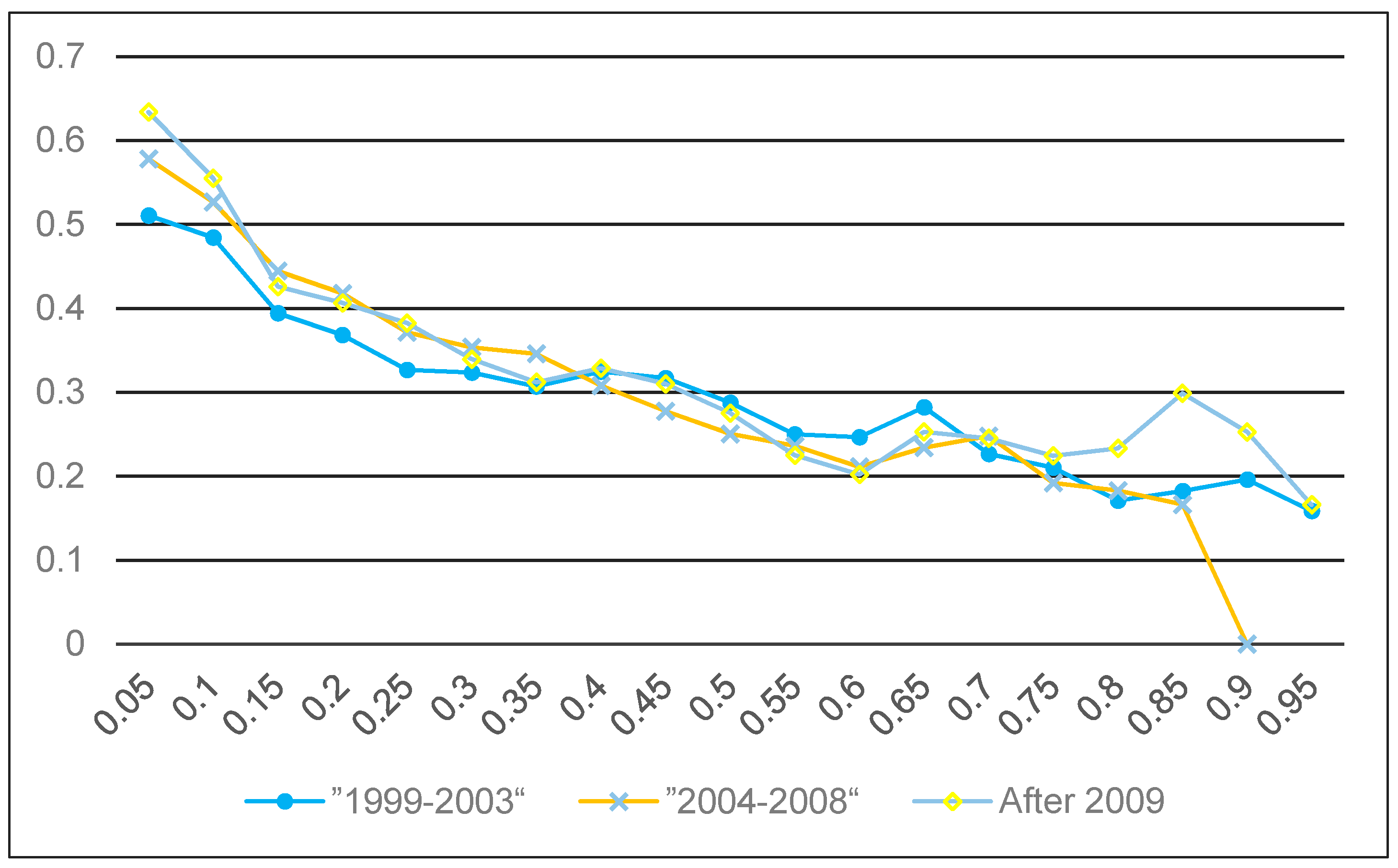
1999–2003	0.329 ***	0.485 ***	0.327 ***	0.288 ***	0.211 ***	0.197 *
2004–2008	0.341 ***	0.526 ***	0.373 ***	0.252 ***	0.195 **	0.133
After 2009	0.398 **	0.556 **	0.383 ***	0.276 **	0.224 *	0.255 *

*** p < 0.001, ** p < 0.01, * p < 0.05.

.

As can be generally observed from the OLS model (Table 3), the time of purchase or construction continues to have a significantly positive effect on housing value after controlling other variables. Compared with individuals who entered the property market before 1998, individuals who entered the property market from 1999 to 2003, 2004 to 2008, and after 2009 have an increased housing value of 39.0%, 40.6%, and 48.9%, respectively. In other words, the later an individual acquires housing, the higher the housing price. This phenomenon can be attributed to the ever-increasing housing price. Due to the ongoing process of China’s market transition, the more fully developed the marketization, the higher the housing value. Hypothesis 4a is thus proven true.

Additionally, such a positive effect varies at different quantile levels. To study the difference and changing trend of the effect in question, a quantile regression coefficient line graph is used. In Figure 1, 19 quantiles are at an interval of 0.05 on the x-axis. There are quantile regression coefficients on the y-axis. Only those regression coefficients with a p-value less than 0.1 are marked.

At the quantile levels from 0.1 to 0.25, which are mainly low-price houses, individuals who enter the real-estate market later obtain higher returns. One possible explanation for this result is that low-price houses are mostly government-subsidized housing units. Due to the commodification reform, houses acquired after 1999 can better satisfy the low-end living needs than before. With the increase of quantile, the value of low-price houses decreases gradually. At the quantile levels from 0.4 to 0.5, the housing value of individuals entering the property market from 2004 to 2008 is slightly lower than that from 1999 to 2003. This result shows that, in the early days of market transition, before a substantial amount of private capital flowed into the property market, the acquisition of middle-end housing could result in some advantages. At the quantile levels from 0.85 to 0.9, a number of high-price houses emerge after 2009 compared with 1998. Such a phenomenon is rare before 2009.

In terms of organizational factor, in

Table 4. Organizational factor of housing price model.

Model Type/Quantile	OLS	0.1	0.25	0.5	0.75	0.9
Work Unit Type
Reference Group: Collective Enterprises
Party and government organs	−0.196	−0.128	−0.206	−0.276 !	−0.169	−0.045
Public institutions, social organizations	−0.291 **	−0.261	−0.335 *	−0.289 **	−0.220 *	−0.181
State-owned enterprises	−0.330 **	−0.427!	−0.414 **	−0.312 **	−0.235 *	−0.15
Private enterprises	−0.281 **	−0.304	−0.332 **	−0.269 **	−0.224 *	−0.194
Self-employed individuals	−0.275	−0.0655	−0.304	−0.299 !	−0.229	−0.299

*** p < 0.001, ** p < 0.01, * p < 0.05, ! p < 0.1.

and Figure 2, the OLS model shows that different work units continue to exert influence on the distribution mechanism of housing, if not a great influence in the redistribution era. Unexpectedly, the housing value of collective enterprises ranks the highest, and the regression coefficients of other enterprises are negative. This is because of the many personal factors under control, and it is different from the results of early empirical studies. Based on the statistics from 1999 [26,36], the income of those from collective enterprises was substantially lower than from private enterprises, the party, and administration organs because collective enterprises were stuck between redistribution and the market. However, in housing distribution in recent years, the identity of collective enterprise has become an advantage rather than a disadvantage. Because party and administration organs do not show significance, and the difference between state-owned enterprises, public institutions, and private enterprises is small, Hypothesis 3a is not directly proven.

Although the difference in the regression coefficients among work organizations is small in the OLS model and at quantile levels from 0.4 to 0.55, the regression coefficient of state-owned enterprises is remarkably lower than other types of organization at the quantile levels from 0.1 to 0.3. In general, the regression coefficient of state-owned enterprises is lower than that of private enterprises. Additionally, the regression coefficient of public institutions is higher than that of state-owned enterprises and lower than that of private enterprises. The p-values of party and government organs, as well as self-employed individuals, are relatively low; thus, an overall pattern is difficult to observe. In general, Hypothesis 3b is proven partly false even though the housing prices of party and government organs and public institutions are higher than those of other organizations at high quantile levels from 0.65 to 0.75; this is illustrative of institutional inertia. However, the regression coefficient of state-owned enterprises ranks the lowest among low-quantile housing, which reflects the brunt of market transition toward old institutional arrangements. As state-owned enterprises have borne most of the brunt, party and government organs and public institutions remain advantageous in middle- to high-price housing.

In terms of human capital factors,

Table 5. Human capital factor of housing price model.

Model Type/Quantile	OLS	0.1	0.25	0.5	0.75	0.9
Education Level
Reference Group: Elementary School and Below
Secondary school	0.325 **	0.283	0.311 *	0.266 **	0.233 **	0.296 **
High school	0.412 ***	0.524 *	0.440 **	0.345 **	0.263 **	0.261 *
University and above	0.584 ***	0.564 *	0.633 ***	0.507 ***	0.471 ***	0.493 ***
Logarithms taken of income	0.233 ***	0.316 ***	0.268 ***	0.270 ***	0.184 ***	0.131 **

*** p < 0.001, ** p < 0.01, * p < 0.05.

and Figure 3 show that, the higher the education level, the higher the housing value. There is a remarkable advantage in college education compared with other levels of education, which corresponds to the conclusion of the OLS model. Therefore, Hypotheses 1a and 1b are proven true. With the increase in quantile, the two variables—income and education level—tend to decrease. This result demonstrates two things. First, as a type of investment, houses, especially high-price houses with a quantile over 0.7, are not directly related to income but related to the investment ability of investors. Second, regarding the acquisition of low-price and middle-price houses with a quantile below 0.65, high-school education has a greater advantage than secondary school education. However, such an advantage becomes less significant when the quantile is over 0.7, and sometimes secondary school education tends to be more rewarding. In terms of human capital, the returns on education mainly differ between individuals with or without a college education. The returns on income are higher in low-value and middle-value houses.

In terms of political capital in

Table 6. Political capital factor of housing price model.

Model Type/Quantile	OLS	0.1	0.25	0.5	0.75	0.9
Occupation
Reference Group: Ordinary Workers
Senior cadre	0.278 *	0.494 *	0.203	0.200 !	0.236 **	0.158
Junior cadre	0.231 !	0.41	0.134	0.182 !	0.176 !	0.250 **
Senior management	0.226 !	0.155	−0.158	0.161	0.223	0.537 *
Junior management	0.245 *	0.236	0.231	0.219 *	0.179 !	0.247
Intermediate and senior technician	0.144 !	0.273	0.0567	0.139 !	0.0942	0.0203
Ordinary technician	0.0382	−0.0529	−0.0257	0.0389	0.0635	0.0896
Organization clerk	0.365 **	0.455 *	0.301 *	0.301 **	0.267 *	0.356 **
Salesman of enterprises and institutions	0.0868	0.161	−0.0476	0.0701	0.0754	0.241
Business service personnel	0.118 !	0.362 *	0.0763	0.0648	0.0316	0.0173
Skilled worker	0.147 !	0.299	−0.0214	−0.0241	0.222 *	0.214 !
Self-employed entrepreneur	0.168	0.121	0.0945	0.135	0.184	0.261
Others	−0.126	−0.212	−0.393	0.323	0.068	−0.205
Party membership	−0.0928	−0.0499	−0.126 *	−0.092	−0.0467	−0.0422

*** p < 0.001, ** p < 0.01, * p < 0.05, ! p < 0.1.

, the housing value of individuals with a title of section chief or above is 32.0% higher than that of ordinary workers, 15.5% higher than that of senior technicians, and 27.8% higher than that of junior management. Hypothesis 2a is thus proven true. Because the p-value of party membership is mostly low and even negative in some quantiles, the influence of party membership on housing value is exerted through other factors, such as occupation, work unit, and education level. When the aforementioned factors are under control, party membership is not as significant as in models with fewer variables. Sometimes, the p-value of party membership in the quantile regression is negative.

The returns of housing value for senior cadre rank are higher than those for junior cadre rank, but the difference is not substantial. The influence and changing trend of political capital in different quantiles can be clearly seen in Figure 4. The occupation variable levels off in different quantiles. However, at the quantile levels from 0.75 to 0.9 and from 0.2 to 0.55, organization clerks have a higher return than other occupations, which has rarely been observed in the literature.

4.2. Housing Added-Value Model

The housing added-value model adopts the same independent variables and methodology as the housing value model. The basic condition of the model and control variables is presented in

Table 7. Basic condition of housing added-value model and control variables.

Model Type/Quantile	OLS	0.1	0.25	0.5	0.75	0.9
Age	−0.00913	−0.013	−0.0041	−0.018	0.00834	−0.00282
Square of age	0.000226	0.000309	0.000216	0.000305 !	0.000017	9.27 × 10−5
Political status	−0.0973	−0.0939	−0.155 *	−0.0935	−0.0736	0.0206
Marriage status	−0.0108	−0.00724	−0.0281	−0.0275	0.0245	0.0134
Family member number	0.0551 **	0.0415	0.0640 **	0.0467 *	0.0536 **	0.0615 *
Gender	−0.0787 *	−0.195 *	−0.112 !	−0.0898 *	−0.0268	0.0177
Province
Reference Group: Shanghai Municipality
Yunnan Province	−1.371 ***	−1.970 ***	−1.526 **	−1.273 ***	−1.212 ***	−1.088 **
Jilin Province	−1.751 ***	−1.854 ***	−1.777 ***	−1.693 ***	−1.697 ***	−1.629 ***
Guangdong Province	−0.648 *	−0.945 **	−0.906 **	−0.766 !	−0.461	−0.28
Henan Province	−1.279 ***	−1.203 ***	−1.241 ***	−1.315 ***	−1.235 ***	−1.357 ***
Gansu Province	−1.568 ***	−1.665 ***	−1.674 ***	−1.492 ***	−1.514 ***	−1.572 ***
Logarithms taken of income	0.229 ***	0.307 ***	0.260 ***	0.264 ***	0.239 ***	0.128 **
Constant term	1.713 **	−0.0158	0.822	1.848 **	1.851 **	3.495 ***
Number of cases	1.560	1.560	1.560	1.560	1.560	1.560
R2	0.533	0.3002	0.3242	0.3623	0.3859	0.3728

*** p < 0.001, ** p < 0.01, * p < 0.05, ! p < 0.1.

.

The coefficient of determination in the OLS model is 0.533, which indicates that the model fits the data well. The model of control variables corresponds to the housing value model.

Regarding time factor, the housing added-value model is different compared with the housing value model. The housing condition from 2004 to 2008 is not significant in

Table 8. Time factor of housing added-value model.

Model Type/Quantile	OLS	0.1	0.25	0.5	0.75	0.9
The Time of Purchase or Construction
Reference Group: Before 1998
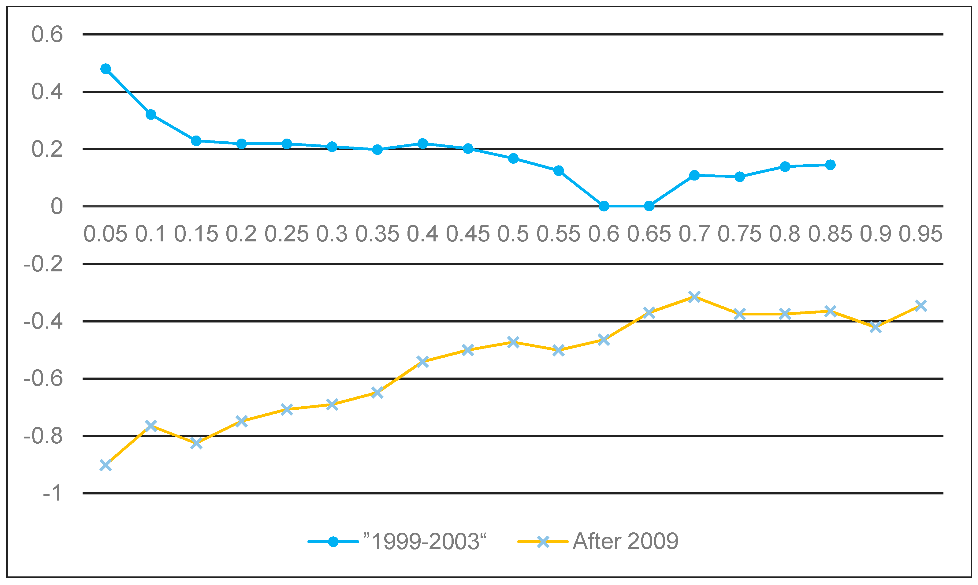
1999–2003	0.195 **	0.320 *	0.218 **	0.165 *	0.102 !	0.123 !
2004–2008	−0.00078	0.155	−0.0199	−0.0915	−0.082	−0.0658
After 2009	−0.478 **	−0.772 **	−0.711 ***	−0.476 ***	−0.376 **	−0.424 ***

*** p < 0.001, ** p < 0.01, * p < 0.05, ! p < 0.1.

. As houses before 1998 were relatively cheap and held for a longer period, new houses after 2009 had a lower added value than those before 1998. However, houses between 1999 and 2003 had a higher added value than houses before 1998. Therefore, Hypothesis 4b has been proven to be partly false.

From the distribution of quantile regression coefficients in Figure 5, small differences are observed in high-return housing after 2009 compared with high-return housing of 1998. This result indicates that low-price housing after 2009 has not fully appreciated and lags behind housing held for a longer time. Another discovery is that housing between 1999 and 2003 had a higher added value than housing before 1998. Taking the historical background into account, 1999 was the starting point of the commodification reform of housing, and premium housing resources that had been prevented from transaction were released into the redistribution system. Therefore, the purchase or construction of property at this time would result in a first-mover advantage. These have become the most value-added properties, even if they are not those selling at the highest price. Such an advantage is most remarkable at quantile levels from 0.05 to 0.15, indicating that, in low-return housing, the added value of purchase or construction from 1999 to 2003 is 23.7% to 61.4% higher than that of purchase or construction before 1998. Due to the commodification of housing, a number of people with low added-value housing have acquired the trading right of housing without much cost, allowing them to gain substantial added-value advantages. Additionally, such an advantage results in 20% more added value in other quantiles and rarely decreases as quantiles increase.

In terms of work unit type, from the overall OLS model in

Table 9. Organizational factor of housing added-value model.

Model Type/Quantile	OLS	0.1	0.25	0.5	0.75	0.9
Work Unit Type
Reference Group: Collective Enterprises
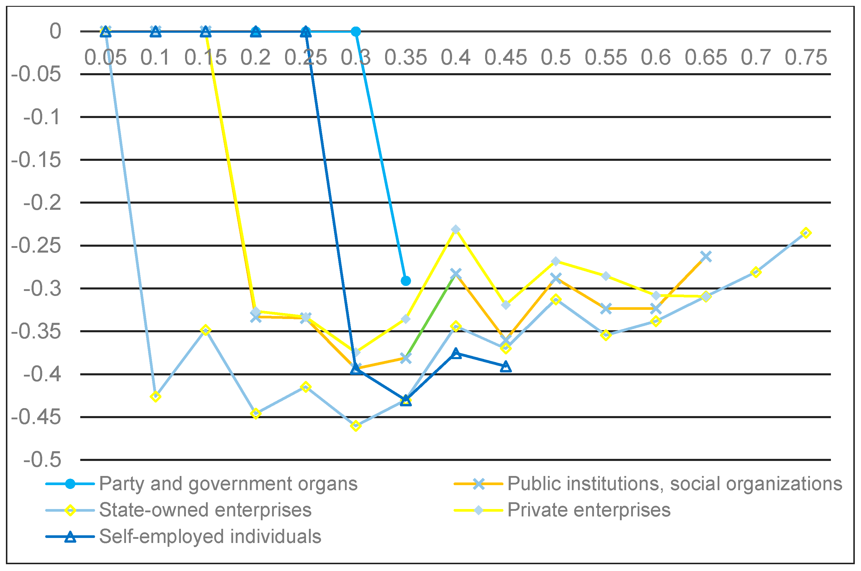
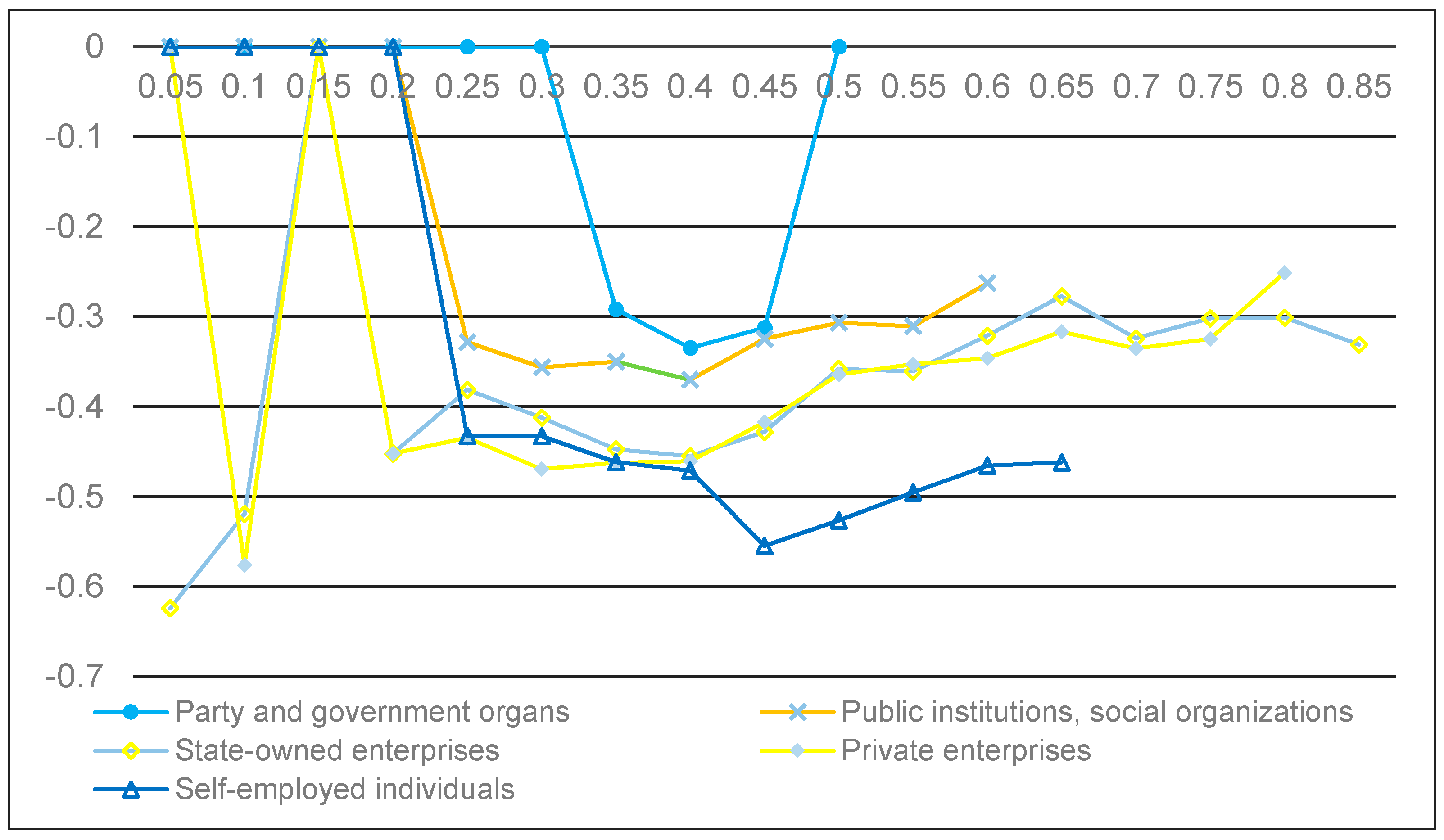
Party and government organs	−0.275 !	−0.0186	−0.204	−0.251	−0.255 *	−0.293 *
Public institutions	−0.324 *	−0.266	−0.329 !	−0.307 *	−0.244 !	−0.212
State-owned enterprises	−0.393 **	−0.521 *	−0.382 *	−0.358 **	−0.303 **	−0.257 !
Private enterprises	−0.409 **	−0.576 *	−0.434 **	−0.365 **	−0.325 **	−0.269 !
Self-employed individuals	−0.446 *	−0.372	−0.433 !	−0.526 *	−0.470 *	−0.423

*** p < 0.001, ** p < 0.01, * p < 0.05, ! p < 0.1.

, collective enterprises have the highest value-added; this is similar to the total housing value model, which followed party and government organs and public institutions. However, the p-value of party and government organs is between 0.05 and 0.1, which is not steady. Regarding the level of added value, the lower the marketization level, the higher the added value. This phenomenon applies to all types of work units except for collective enterprises. In other words, the work units that do not have a fully developed marketization similar to party and government organs and public institutions tend to have higher added value. After considering the exception of collective enterprises, Hypothesis 3b is proven to be partly true.

From the changing pattern of quantile regression coefficients in Figure 6, a similar pattern can be observed. The group of self-employed individuals is the work unit type with the highest level of marketization and the lowest added value. In quantiles after 0.45, the middle- and high-return housing with high added value do not fit into the group of self-employed individuals. Although there is a breakpoint in coefficients of party and government organs, these factors remain advantageous in low- and middle-return housing on quantile levels from 0.35 to 0.45. The income of non-corporate organizations, such as party and government agencies and public institutions from real-estate appreciation, is between 0.25 and 0.85 points, which is greater than private and state-owned enterprises. In general, in housing quantiles with higher returns, the difference between non-enterprise organizations and collective enterprises tends to be smaller.

Regarding the human capital factor, from the OLS model in

Table 10. Human capital factor of housing added-value model.

Model Type/Quantile	OLS	0.1	0.25	0.5	0.75	0.9
Education Level
Reference Group: Elementary School and Below
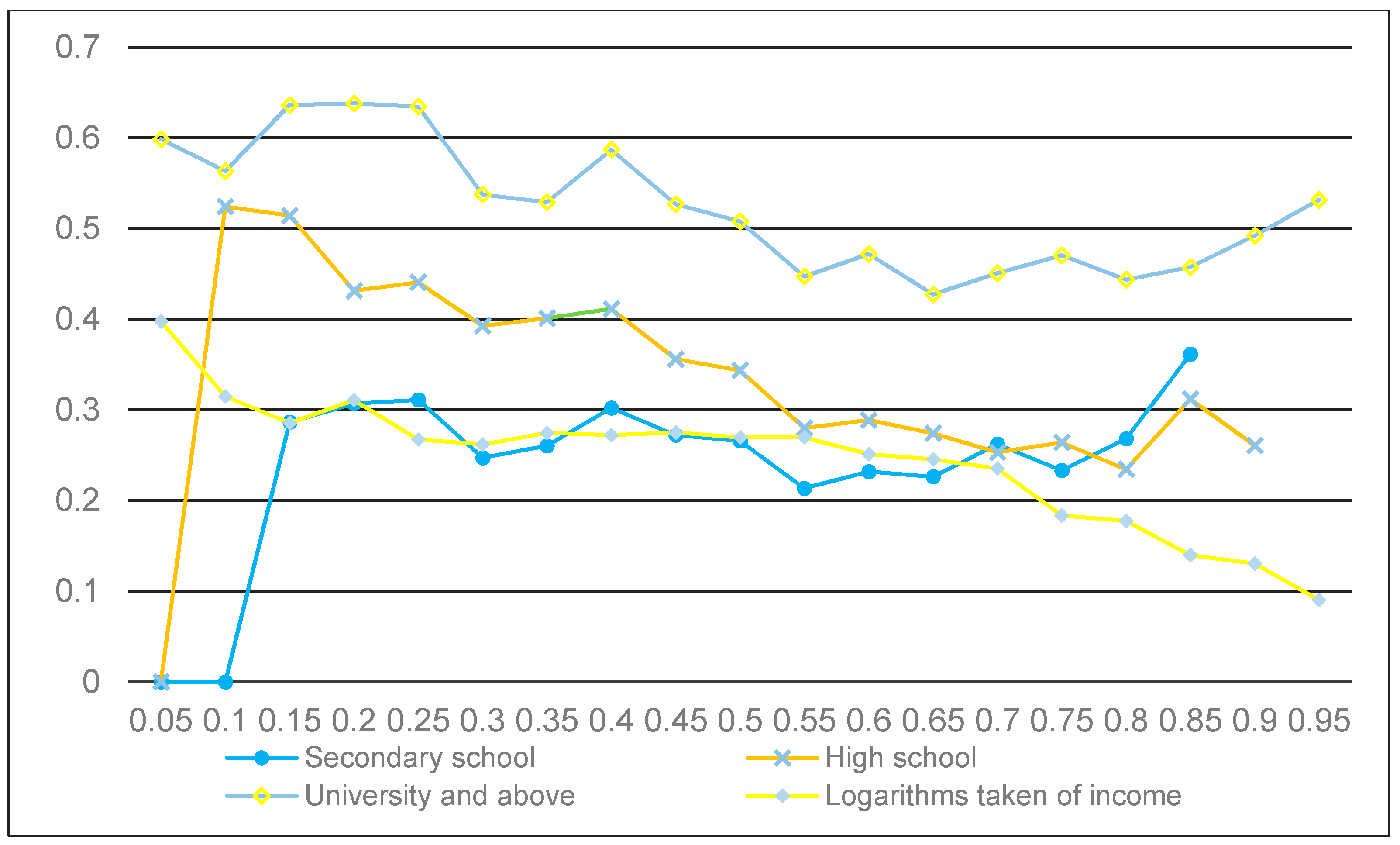
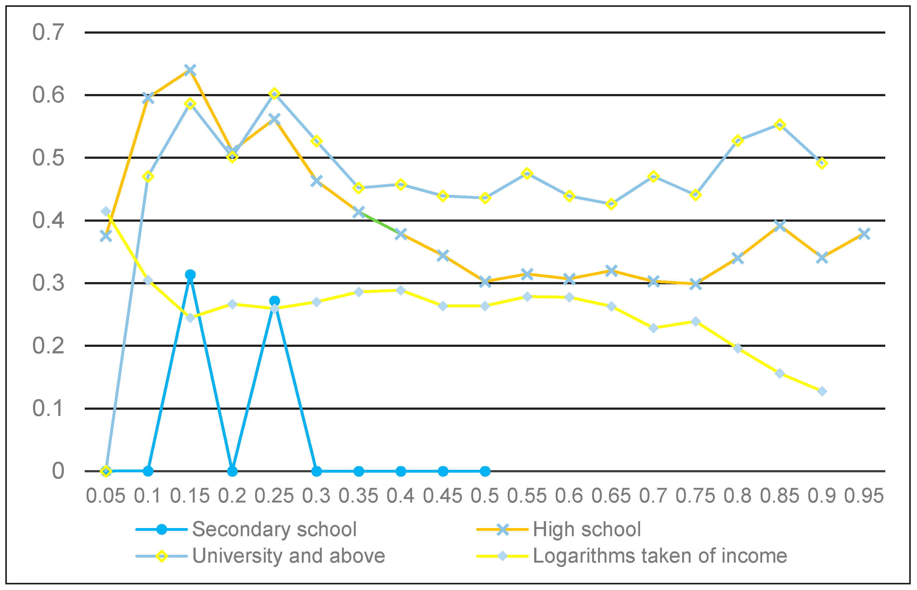
Secondary school	0.291 *	0.215	0.270 !	0.189	0.327 **	0.370 **
High school	0.460 ***	0.596 **	0.562 **	0.302 *	0.298 **	0.342 **
University and above	0.521 ***	0.470 *	0.604 **	0.436 **	0.441 ***	0.493 ***
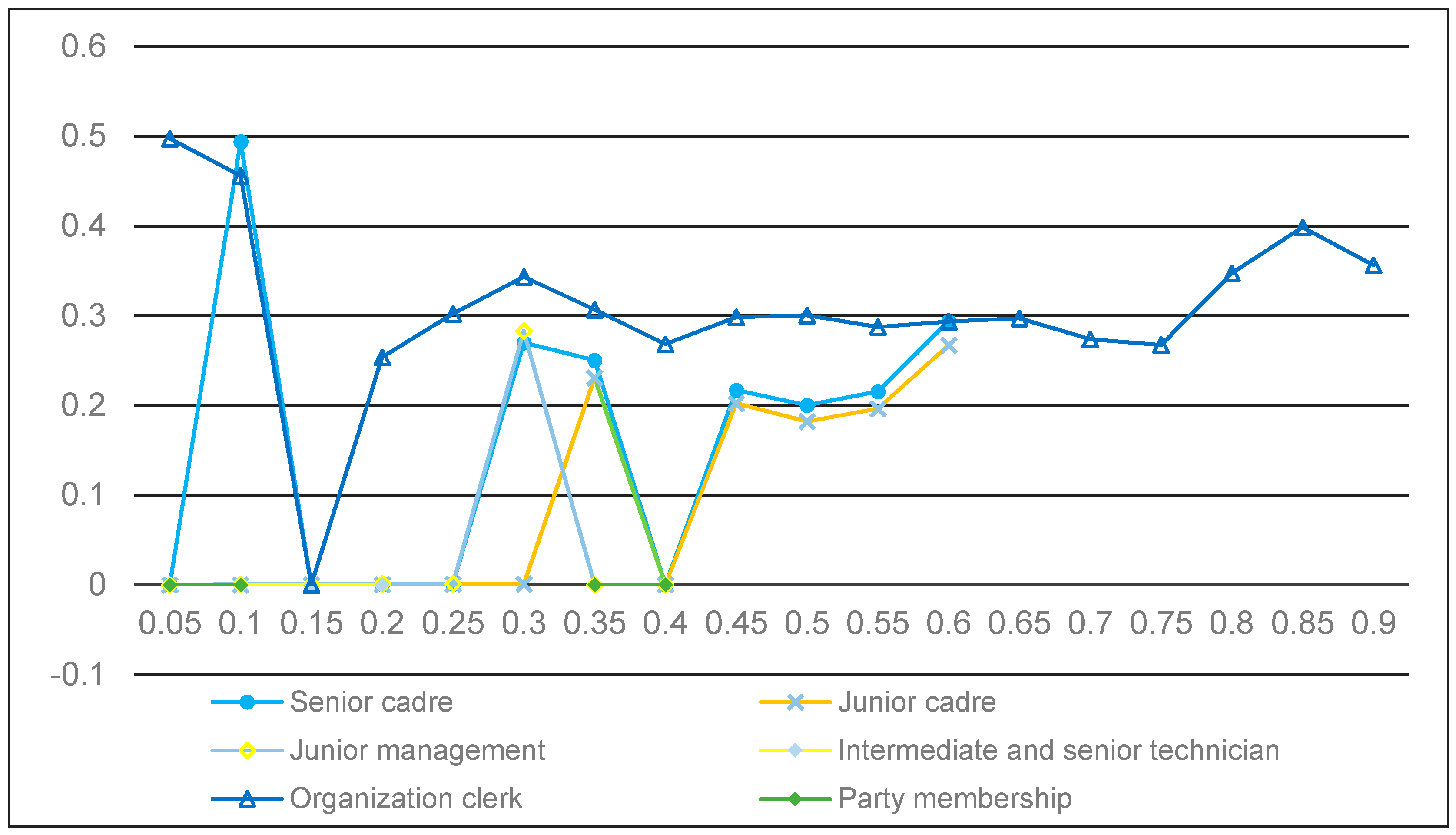
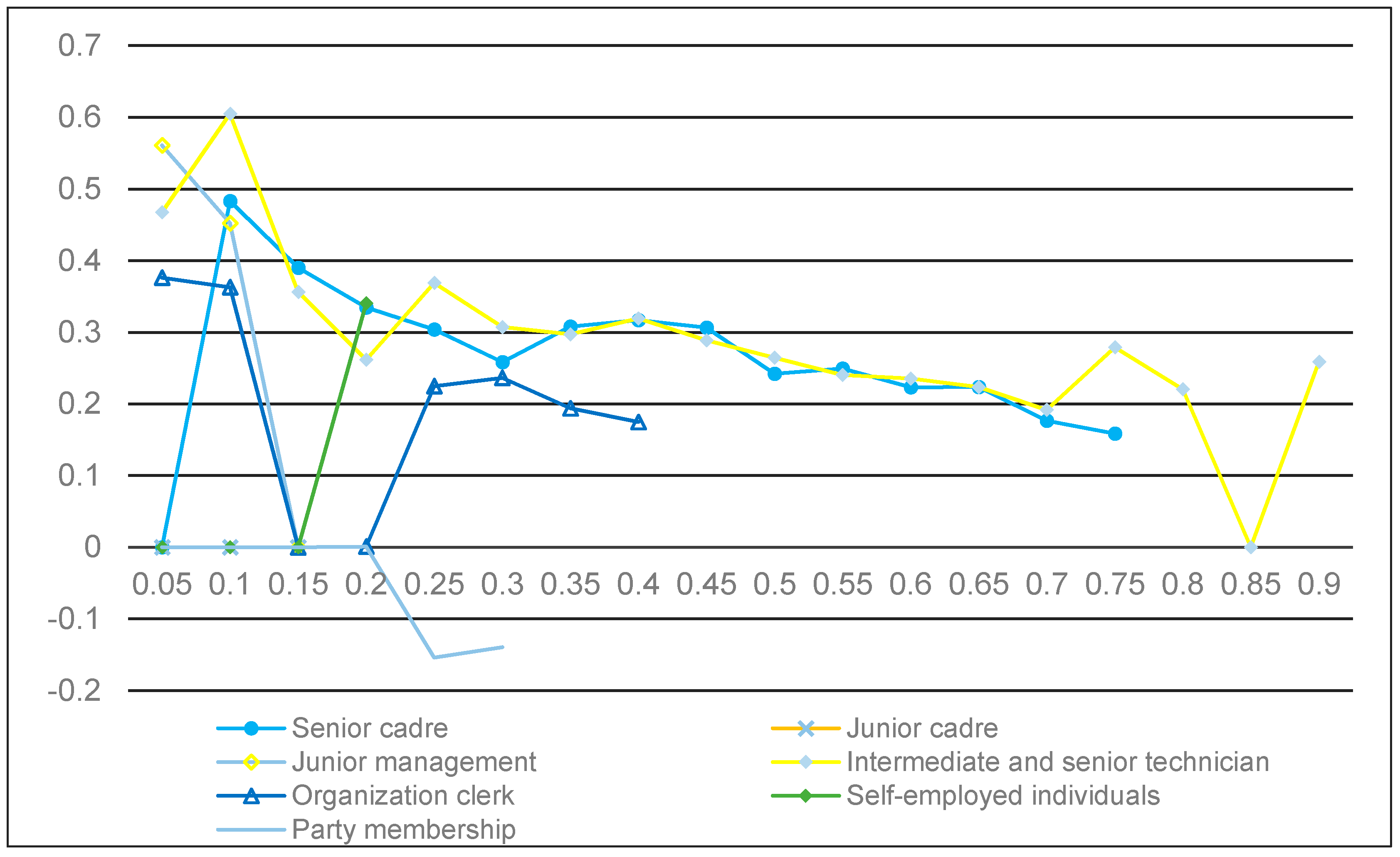
Senior cadre	0.301 *	0.482 !	0.303 *	0.243 *	0.158 !	0.117
Junior cadre	0.148	0.248	0.194	0.109	0.048	−0.0077
Logarithms taken of income	0.229 ***	0.307 ***	0.260 ***	0.264 ***	0.239 ***	0.128 **

*** p < 0.001, ** p < 0.01, * p < 0.05, ! p < 0.1.

, the higher the education level, the higher the income and the higher the housing added value. However, the advantage of a college education is less remarkable than it is in the housing value model. The housing added value of high-school education and college education is 68.3% and 58.4% higher, respectively, than elementary school education and below.

In the quantile regression model in Figure 7, the added value of college education is higher than that of other education levels at high quantile levels from 0.6 to 0.95. At low-quantile levels from 0.05 to 0.35, the difference between college education and high-school education is not substantial. The added value of high-school education is even higher than that of college education, which probably reflects that the human capital factor plays an insignificant role in low-return housing. Therefore, high-school education can also result in high returns on low-return housing. However, college education is a must to gain returns on high-return housing. With the increase in quantiles, the influence of income on housing added value decreases, which is the same as in the housing price model.

In

Table 11. Political capital factor of housing added-value model.

Model Type/Quantile	OLS	0.1	0.25	0.5	0.75	0.9
Occupation
Reference Group: Ordinary Worker
Senior management	0.255	0.339	0.269	0.101	0.198	0.33
Junior management	0.214	0.412	0.270 !	0.11	0.0392	0.0763
Intermediate and senior technician	0.176 !	0.452 *	0.0507	0.178	0.103	−0.0691
Ordinary technician	0.0294	0.119	−0.0687	0.083	0.0638	−0.0609
Organization clerk	0.372 **	0.604 **	0.368 **	0.265 *	0.278 *	0.256 *
Salesman of enterprises and institutions	0.138	0.28	0.0814	0.133	0.0808	−0.0676
Business service personnel	0.157 **	0.363 !	0.224 *	0.118 !	0.0847	−0.0145
Skilled worker	0.126	0.351	−0.162	0.0261	0.0939	0.0748
Self-employed entrepreneur	0.214	0.341	0.321 *	0.237	0.119	0.122
Others	0.195	1.059 **	0.48	0.329	0.152	−0.118
Party membership	−0.0973	−0.0939	−0.155 *	−0.0935	−0.0736	0.0206

*** p < 0.001, ** p < 0.01, * p < 0.05, ! p < 0.1.

, any variables in occupation and political capital factor are not significant, but the returns of organization clerks still rank the highest in terms of housing added value. The difference between the occupation of section chief and above and the occupation of organization clerk is smaller than that in the housing price model. The housing added value of section chief and above and organization clerk is, respectively, 35.1% and 44.9% higher than that of an ordinary worker.

In the quantile model in Figure 8, the p-value of party membership is partly negative at the low and middle quantile levels, which is similar to the housing value model. Therefore, Hypothesis 2b is proven to be partly false. The difference in the returns among various occupations is not large and decreases with the increase in quantiles. However, in the housing price model, the regression coefficients of various occupations in different housing prices are more or less steady. This result indicates that a negative correlation between the returns from the high-return property market and occupation, which is especially remarkable at quantile levels from 0.1 to 0.25.

5. Conclusions and Discussion

5.1. Conclusions

The research results show that human capital exerts significant influence. Individuals with a high education level are more likely to acquire high-value housing, especially individuals with a college education. Additionally, individuals with a high education level are more likely to profit from the added value of housing. However, a small difference was observed between individuals with a college education and individuals with a high-school education regarding low added-value housing. Individuals with low-quality and low-return housing profit more from factors such as education and income. Therefore, improving education level remains a reliable means to reduce housing inequality, especially for individuals comprising the lower classes. We found that political capital exerts less influence. When a cadre position is considered as a type of occupation, it does not result in the greatest returns, and the returns of an organization clerk outweigh those of cadres with a title of section chief or above. Party membership may exert influence through other variables. When other variables are under control, party membership even plays a negative role under some circumstances. The influence of political capital on the distribution of housing is not as strong as it was before. In the property market, the quantiles of state-owned enterprises are not as significant as those of private enterprises, and this indicates that traditional work organizations have borne the brunt of market transition. Although collective enterprises rank the highest in returns on the property market, non-enterprise organizations are better than enterprises in terms of housing added value. This result shows that the redistribution system of the work unit era has a substantial effect on current housing inequalities, and patience is required as the marketization process plays out. The later an individual acquires housing, the higher the housing value; however, this phenomenon does not mean that the longer an individual holds the property the higher the added value. The housing added-value returns of individuals who entered the property market from 1999 to 2003 are not only greater than individuals entering after 2009, but also greater than individuals owning a house before 1998. This is why first-mover advantage is critical in the early days of market transition.

5.2. Discussion

From its genesis, China’s market reform has been guided and intervened in by the government. In contrast to the “shock therapy” of the drastic changes in Eastern Europe, China’s gradual reforms are carried out under the action of improving the socialist system and exerting the institutionalization of socialism. This is the continuity of the political system and reality [37] (Liu 2003). The current social and economic state of China is not a completely self-disciplined market economy system, and all irrational interventions, including interventions of power and privileges, have not all been driven out of the market system [38,39].

On one hand, in the field of market economy, emerging economic elites have gradually emerged whose privileges are based on asset ownership. On the other hand, cadres, or at least some of them, have also learned how to use the market and successfully transfer their own bureaucrats. Privileges are therefore “commercialized” [40] (Szelenyi, 1987). This dual stratification system is particularly obvious in the housing field. On the one hand, according to the logic of market operation, housing resources are differentiated based on an individual’s financial ability, and the market provides more incentives for direct producers. Market incentive mechanisms will reflect the return of human capital indicators, such as education, skill level, and housing resources. On the other hand, the powerful elite in the original redistribution system not only use the “privatization of public housing” reform process to share advantages under the planned economic system, as housing resources are legally “privatized” and “commercialized”, but they also seize favorable political opportunities in the housing reform process or seek housing benefits through administrative power to enjoy market privileges.

While market transition theory and power continuance theory have a common assumption that China is undergoing a long process of marketization, the common concern of the two theories is how new resources resulting from the market transition are used and divided. Market elites gain resources fairly with better human capital. Powerful elites gain resources by transforming previous power advantages into market ability and status. The possible problem of such an assumption is that the speed of resources emerging from the market transition is misinterpreted into a steady speed, and a fight over resources between market elites and powerful elites is based on an unchanging number of resources.

However, when the time factor is included in this research, the speed of resources emerging from the market transition is unsteady. In the early days of market transition, such resources tend to emerge in a substantial number. Housing acquired between 1999 and 2003 has the highest added value in the housing market. This result means that the question of which party occupies the new resources first is not as critical as the question of which party first gains access to the new resources. An example of this is housing inequality. Once an individual acquires premium housing early, she or he has the capability to increase added value in the long term and profits from renting the house, deepening the stratification and forming a greater Matthew Effect. The answer to this can be found in the fundamental debate of market transition: which party can gain access to the new resources the earliest?

Based on the advantage of collective enterprises and organization clerks on housing value and housing added value, this paper proposes a third approach to answering the above question. Greater human capital and political capital do not necessarily result in more market resources. However, the work units between the market and redistribution system, such as collective enterprises, and occupations, such as organization clerk, which can directly participate in the housing redistribution process deliver the highest housing returns. Although collective enterprise did not have substantial advantages in the early days of market transition, collective enterprise is likely to profit from its vague identity between the market and redistribution system in the long process of reform. Organization clerks can profit because of their early and direct contact with the distribution of housing. These two show the competitive advantage outside the binary contrast between the market and redistribution. Regardless of which main resource distribution system is chosen, it is possible to bypass or avoid these two and then gain specific advantages. A prediction for this process is that, if such a possibility were not managed properly, a troubling group that could neither be affected nor directly influenced by marketization might emerge, further compounding the issue of housing inequality in the long term.

References

- Wang, F.; Ma, L. Boundaries and Categories: Rising Inequality in Post-Socialist Chin; Zhejiang People’s Publishing House: Hangzhou, China, 2013. [Google Scholar]
- Reuters Beijing. The First Time the Bureau of Statistics Released Gini Coefficiet in China. Available online: http://cn.reuters.com/article/cn-gini-population-reform-idCNCNE90H04A20130118 (accessed on 25 October 2021).
- Davis, D.S. Urban Chinese homeowners as citizen-consumers. In The Ambivalent Consumer edited by Sheldon Garon and Patricia Maclachlan; Cornell University Press: Ithaca, NY, USA, 2006; pp. 281–299. [Google Scholar]
- Davis, D. Urban consumer culture. China Q. 2005, 183, 692–709. [Google Scholar] [CrossRef] [Green Version]
- Gan, L. China Household Finance Survey Report; Southwestern University of Finance and Economics Press: Chengdu, China, 2012. [Google Scholar]
- Merton, R.K. The matthew effect in science, ii: Cumulative advantage and the symbolism of intellectual property. Isis 1988, 79, 606–623. [Google Scholar] [CrossRef] [Green Version]
- Walder, A.G. Property rights and stratification in socialist redistributive economies. Am. Sociol. Rev. 1992, 57, 524–539. [Google Scholar] [CrossRef]
- Parish, W.L.; Ethan, M. Politics and markets: Dual transformations. Am. J. Sociol. 1996, 101, 1042–1059. [Google Scholar] [CrossRef]
- Gerber, T.P.; Hout, M. More shock than therapy: Market transition, employment, and income in russia, 1991–1995. Am. J. Sociol. 1998, 104, 1–50. [Google Scholar] [CrossRef]
- Bian, Y.; Logan, J.R. Market transition and the persistence of power: The changing stratification system in urban china. Am. Sociol. Rev. 1996, 61, 739–758. [Google Scholar] [CrossRef]
- Zhou, X.G. Economic transformation and income inequality in urban china: Evidence from panel data. Am. J. Sociol. 2000, 105, 1135–1174. [Google Scholar] [CrossRef]
- Bian, Y.J.; Zhang, Z.X. Marketization and income distribution in urban china, 1988 and 1995. Res. Soc. Strat. Mobil. 2002, 19, 377–415. [Google Scholar] [CrossRef]
- Walder, A.G. Communist Neo-Traditionalism; University of California Press: Auckland, CA, USA, 1988. [Google Scholar]
- Bian, Y.; Liu, Y. Social stratification, home ownership, and quality of living: Evidence from china’s fifth census. Sociol. Res. 2005, 3, 82–98. [Google Scholar]
- Liu, X. Market transition and social stratification: Theoretial debates and further research issues. Soc. Sci. China 2003, 5, 102–110. [Google Scholar]
- Liu, Z.; Hu, R. Urban housing stratification: An analysis based on cgss2006 data. Chin. J. Sociol. 2010, 30, 164–192. [Google Scholar]
- Nee, V. Social inequalities in reforming state socialism: Between redistribution and markets in china. Am. Sociol. Rev. 1991, 56, 267–282. [Google Scholar] [CrossRef] [Green Version]
- Nee, V. The emergence of a market society: Changing mechanisms of stratification in china. Am. J. Sociol. 1996, 101, 908–949. [Google Scholar] [CrossRef]
- Szelenyi, I. Social inequalities in state socialist redistributive economies. Int. J. Comp. Sociol. 1978, 19, 63–87. [Google Scholar] [CrossRef]
- Chen, Z. Market transition or power conversion: The wealth distribution and the regional disparity of urban residents in mainland china. In Market, Classes and Politics: Chinese Society during Transition; Liu, Z., Ed.; Hong Kong Institute of Asia-Pacific Studies, The Chinese University of Hong Kong: Hongkong, China, 2000. [Google Scholar]
- Walder, A.G. Local governments as industrial firms: An organizational analysis of china’s transitional economy. Am. J. Sociol. 1995, 101, 263–301. [Google Scholar] [CrossRef] [Green Version]
- Liu, X. Housing inequality in urban china. Sociol. Forum Fudan Univ. 2005, 1, 149–171. [Google Scholar]
- Xie, Y.; Hannum, E. Regional variation in earnings inequality in reform-era urban china. Am. J. Sociol. 1996, 101, 950–992. [Google Scholar] [CrossRef]
- Liu, Z.Q. The economic impact and determinants of investment in human and political capital in china. Econ. Dev. Cult. Change 2003, 51, 823–849. [Google Scholar] [CrossRef]
- Song, S.G. The delayed effect of power conversion-an explanation of the regeneration and circulation of elites in the process of transforming socialist countries to markets. Sociol. Res. 1998, 3, 26–36. [Google Scholar]
- Li, B.; Walder, A.G. Career advancement as party patronage: Sponsored mobility into the chinese administrative elite, 1949–1996. Am. J. Sociol. 2001, 106, 1371–1408. [Google Scholar] [CrossRef] [Green Version]
- Fan, G.; Wang, X. Marketization index for China’s provinces. Econ. Res. 2003, 3, 9–18. [Google Scholar]
- Li, S.; Wei, Z.; Ding, S. Empirical analysis on the inequality and the reason for china’s residents’ property distribution. Econ. Res. J. 2005, 6, 4–15. [Google Scholar]
- Zhang, J. Study on the Housing Inequality in China; Dongbei University of Finance and Economics: Dalian, China, 2013. [Google Scholar]
- Hu, R. Housing inequality during market transition: Analysis of housing value and housing quantity. J. Gansu Admin. Ins. 2014, 6, 108–116. [Google Scholar]
- Li, B. Housing Policies in Differentiatio; Social Sciences Academic Press: Beijing, China, 2009. [Google Scholar]
- Luo, C.L. Housing area inequality in urban residents: An analysis based on 2000 and 2005 census in chin. Acad. Bras. 2014, 1, 80–90. [Google Scholar]
- Hu, R. Housing inequality during the market transition: Evidence from the data of cgss2006. Soc. Chin. J. Sociol. Shehui 2012, 32, 126–151. [Google Scholar]
- Wu, X.B. Gains and Losses of Economic Reform in the Course of History; Zhejiang University Press: Hangzhou, China, 2013. [Google Scholar]
- Zhou, F.Z. Fiscal Relations and Local Governance; Shanghai SDX Joint Publishing Company: Shanghai, China, 2012. [Google Scholar]
- Xie, Y.; Wu, X. Danwei profitability and earnings inequality in urban china. China Q. 2008, 195, 558–581. [Google Scholar] [CrossRef] [Green Version]
- Liu, X. Market transformation and social stratification: The focus of theoretical debate and problems to be studied. Chin. Soc. Sci. 2003, 102–110. [Google Scholar]
- Giddens, A. The Class Structure of the Advanced Society; Hutchinson: London, UK, 1973. [Google Scholar]
- Goldthorpe, J. Social Mobility and Class Structure in Modern Britain; Clarendon: Oxford Shire, UK, 1987. [Google Scholar]
- Szelnyi, I.; Manchin, R. Social policy under state socialism: Market, redistribution, and social inequalities in East European socialist societies. In Stagnation and Renewal in Social Policy; Rein, M., Esping-Anderson, G., Rainwater, L., Eds.; M.E. Sharpe: White Plains, NY, USA, 1986; pp. 102–139. [Google Scholar]