The Effect of Ageing, Gender and Environmental Problems in Subjective Well-Being

Abstract

This paper studies the relationship of factors such as ageing, gender and environmental problems included in the quality of life (QoL) with the subjective well-being represented by the life satisfaction (LS) indicator of the citizens of 33 European countries. To do so, it uses the LS of a country’s citizens as the dependent variable; ageing, gender and environmental variables as independent variables; and other factors included in the QoL indicators and macroeconomic factors as control variables. Analysis uses data from the World Values Survey (WVS) and the European Values Study (EVS) for LS, from Eurostat for QoL indicators and World Bank for macroeconomic indicators. The values of LS have been treated based on the individual data from WVS and EVS in percentages according to their levels by country, and we present four robust models (two logit model and two OLS model). The results show that arrears of people aged 65 and over are a relation of positive significative in models with low levels of LS. The opposite is true for the income of people aged 65 and over. On the other hand, pollution, grime or other environmental problems and inequality show an inverse relationship with life satisfaction in models with high levels of satisfaction and a positive relationship in models with low levels of satisfaction. Nonetheless, the study has also shown contradictions in the gender gap and poverty indicators that should be studied further.

1. Introduction

Every day, it is more usual to find citizens’ well-being among the main objectives of the governments of developed countries and many international organizations. According to some authors, there is a belief that objective well-being (such as wealth) should be part of the overall indicator of well-being, and that GDP by itself is not adequate to describe the well-being of a country. In contrast, wealth on its own is not sufficient to describe a person’s happiness [1]. The individual well-being of the citizens of a country “is highly subjective and person-specific, and thus policies should focus on making well-being possible by providing the freedoms and capabilities that allow each person to achieve what will contribute to his or her own well-being” [2] (p. 65). In that sense, the same thing happens with life satisfaction and happiness. The individual subjectivity of these variables makes it necessary to use polls for this study [3]. Among the most important surveys that include data on life satisfaction and happiness are the World Values Survey (WVS) and the European Values Study (EVS).

Many countries and researchers use psychological well-being, health, education, time use, cultural diversity and resilience, good governance, community vitality, ecological diversity and resilience, and living standards as measures of happiness or LS [4,5,6]. Many of the dimensions coincide with those considered by Eurostat and will be discussed in this study. Among them, there are four variables (income, wealth, civic commitment and governance) that report the highest quality of life indicators and the highest degree of happiness, and others (homicide rates, housing without basic services, poor working conditions and pollution) that present an inverse relationship with well-being [7].

Unlike life satisfaction and happiness, quality of life presents objective situations and subjective perceptions that combine to determine an individual’s well-being [8]. Currently, there is an accepted consensus on the importance of both dimensions for the study of well-being. The QoL indicators are included such as objective income, and others, such as LS, that are entirely subjective. Among these measures of quality of life are the ones published by the OECD Better Life Index, which includes a total of 11 dimensions that are materialized in 24 indicators including five subjective indicators, one of which is LS and that is presented by the European Statistical System with nine dimensions: material living conditions, productive or other main activity, health, education, leisure and social interactions, economic security and physical safety, governance and basic rights, natural and living environment and overall experience of life. In this work, we will focus on the effect of some indicators that make up the European Statistical System’s QoL on satisfaction with life from the World Values Survey (WVS) and the European Values Study (EVS). This work focuses especially on those indicators related to ageing, gender employment gap and the environment, and based on the studies analyzed on subjective well-being, other quality of life and macroeconomic indicators have been used as control variables. The LS indicator has been selected to reflect citizens’ well-being since it is more stable over time to measure well-being [9]. In Pavot and Diener study, it showed a degree of the temporal stability of 0.54 for four years.

There are differences in studies between income and well-being. Higher incomes than others report higher levels of happiness [10], although dissatisfaction with income occurs when what you want exceeds what you get and when people feel they deserve more than they earn [11]. Other studies show that people with higher income tend to be happier. Still, as income increases, happiness does not increase in the same way [4] as higher-income aspirations reduce life satisfaction [12].

On the other hand, among the European Statistical System’s QoL factors, there are also labour variables such as employment, unemployment, quality of work, inactivity and gender inequality. Unemployment and employment affect not only people’s economic situation but also their social environment [13]. Employment causes an increase in subjective well-being. Just as it provides for the development of a person and acquiring new skills and knowledge, it makes people feel less monotonous and routine [14]. Temporary employees have generally lower job satisfaction, although it depends on the type of contract and job security [15]. Job loss and the resulting period of unemployment can lead to a high degree of stress, causing impacts on people’s identities, depression due to the economic situation and the lack of satisfaction [16,17].

Unemployment affects people’s social lives; their consumption patterns are altered, they show symptoms of isolation, loss of self-esteem, feelings of hopelessness that can lead to the deterioration of their physical well-being producing a prolonged duration of this state and an increase of negative emotions, which affect their mental health. Another relevant aspect is that the longer the duration and repetition of unemployment, the greater the dissatisfaction. Women, during the reaction process, once they were unemployed, presented fewer negative reactions than men. Similarly, repeated unemployment did not mean that responses were better [18]. It also affects the well-being of those close to you. The existence of high unemployment makes being employed difficult. Therefore, a key factor for well-being is the security of the labour market. Job instability affects men more than women [19].

It is difficult to find indicators that measure the effects of the gender gap on women’s well-being [20]. Housework is mainly carried out by women, which prevents women’s full incorporation into the labour market and affects women’s well-being [21,22]. Therefore, the gender gap negatively affects the well-being of women [23]. More women than men are in the inactive population, although most of the existing studies on the inactive population focus on retirees.

The effect of retirement is positive with life satisfaction, but not to the same degree whether you are employed or unemployed at the time of retirement. The level of satisfaction with life when retiring is higher in employed people than in an unemployed person. Although, the well-being of the involuntarily unemployed increases considerably upon retirement [24,25]. Moreover, going from a work situation to being permanently ill implies lower levels of psychological well-being [26]. The psychosocial quality of labour and mental health is related to people’s subjective well-being [27].

Physical and psychological well-being are also essential factors for well-being. The existence of a direct relationship between physical activity and well-being and inverse with sedentary behaviour has been proven [28,29,30]. Although [31] show that health does not directly affect the satisfaction of the quality of life in general but instead has an indirect effect on health satisfaction, [32] clarifies and indicates that the relative importance of satisfaction with one’s health for QoL depends on the QoL measures used. For this author, people may perceive health as an essential factor about other vital areas of life. Still, satisfaction with their health may not necessarily be the most important determining factor in satisfaction with other critical life areas. In addition, a negative relationship has been confirmed between living in a deficient dwelling and health status [33].

Educational level also influences well-being; “Those individuals with a higher level of education are characterised by lower levels of emotional and physical distress than those with a lower level of education; those with higher levels of depression and discomfort among others; and who have lower levels of pleasure, hope, happiness, energy and physical fitness than more educated individuals. The latter is not satisfied with their work” [14] (p. 275). There is a positive relationship of educational level with QoL, associating secondary and tertiary education with a better quality of life [34,35].

Ageing, economic insecurity, payment arrears and physical safety also affects well-being. The first signs of ageing usually appear in people over 50 years of age and can negatively impact the individual’s functioning in society and interpersonal relationships [30,36,37]. It has also been found that the life satisfaction of elderly people living in social housing is very low and that moving to better housing increases life satisfaction [38]. The economic insecurity and payment arrears contribute to reducing the well-being and health of households. Mortgage arrears are an additional burden on households facing financial difficulties, making it a social problem. They can cause health problems and homelessness, with indirect effects on state finances [39]. The frequency of arrears is relevant, as the occasional incidence had a significantly lower impact [40].

The relationship between well-being and physical safety has also been analysed. Life satisfaction is lower for victims and people who lived in areas with higher crime rates. Property crime (theft) affects all household members equally. The real nature of a murder is related to the quality of life perceived by the respondent [41]. The negative effects of both property crimes and homicides may be similar among all existing household members, making the perceived quality of life a valid measure of crime victimisation’s well-being impact. Overall, all crimes and high crime rates reduce life satisfaction, and assaults quadruple the negative relationship with QoL, compared to robberies [42,43]. Personal well-being is more affected by fear of crime than by being a victim [44].

Environmental variables such as pollution, noise, and other environmental problems are also among the European Statistical System’s QoL factors. Air pollution is a global health and environmental problem, especially in major developing countries [6,45]. There is consensus on a negative relationship between air pollution and satisfaction with life. There is also a binding relationship between well-being, income and air pollution concerning air quality [46] and negative effects on the cardiovascular and respiratory systems [47]. The exposure to PM10 may not have a direct health effect. Deficient air pollution levels can reduce subjective well-being and manifest itself through irritation, discomfort or high physical stress [48]. Besides, it directly influences people’s lives through their visual perceptions, reducing their subjective well-being [6]. Climate change will have effects on physical and mental health and well-being. It is expected that extreme storms and droughts will occur, and this will result in human beings experiencing both short and long term decreases in quality of life, presenting: anxiety, depression, post-traumatic stress, substance abuse and even suicides [49].

These studies open a new path for us on the need to elaborate policies that pursue growth and development and consider the sustainability and well-being of citizens. For this reason, this work focuses on how the indicators of ageing, gender and environment included in the set of QoL indicators according to Eurostat affect the LS of citizens. This paper’s main objective is to increase our understanding of the impact on life satisfaction of the environmental and social situations that affect the citizens of the 33 countries analysed, and the combined effects of these variables. To achieve this, we have used information from individual WVS and EVS surveys covering 33 countries from 1999 to 2018 and calculated the percentage of citizens per country in the ten levels of satisfaction with life that these surveys include. We tested four relationships by constructing the LS dependent variable differently for each, and two models were built.

The contribution of this work is to study the effect of QoL factors such as ageing, gender and environment issues of the European Statistical System on life satisfaction of citizens using several specifications based on the LS index as a dependent variable and using other QoL and macroeconomic indicators as control variables in order to visualize the results with different treatments of the life satisfaction variable and to deepen the study of these variables. We have found it appropriate to focus our research on these four different approaches to one variable—satisfaction with life (LS), which contains ten levels, and explore it using different models. We used these models to test the following hypotheses:

• H1: Countries with a higher percentage of the population aged 65 and over who have arrears (mortgage or rent, utility bills or hire purchase) present a higher percentage of citizens with low levels of LS (1–5).
• H2: As income increases for people aged 65 and over, the percentage of people with life satisfaction levels of 8 or above increases.
• H3: Increasing the percentage of the population aged 65 and over who perceive their health as “very good” raises the probability that a country will have more than 35% of its population at satisfaction levels 9 and 10.
• H4: Countries with a higher percentage of gender employment gap are more likely to have more than 25% of their population with LS levels from 1 to 5 than those with less gender employment gap.
• H5: Air pollution, noise from neighbours and other environmental problems have an inverse relationship with the percentage of citizens in countries with an LS level equal to or greater than 8.

2. Materials and Methods

Like many other studies on happiness and satisfaction with life, this work has used the World Values Survey (WVS) databases, European Values Study (EVS), Eurostat and the World Bank. The WVS and EVS databases provided data on the dependent variable, satisfaction with life. Both sources could be used as the WVS website indicates that interested users in European countries study EVS WVS’s features [50,51,52,53]. The data obtained comes from citizens of 33 countries at the individual level. Eurostat provided the QoL indicator data and the World Bank the macroeconomic data on the countries under study. All previous data sets were entered into Stata statistical software (version 16) for analysis.

Previously, we have established the reasons for selecting life satisfaction as a variable to study subjective well-being and different indicators of quality of life and macroeconomics as independent and control variables. Some studies focused on these relationships, but this study goes further because it shows other models depending on the LS indicator’s treatment. For this, the dependent variable (LS) has been constructed in four different ways using data from hundreds of surveys carried out between 1999 and 2018 by the World Values Survey and European Values Study groups in 33 countries to calculate the percentages by levels.

(1)

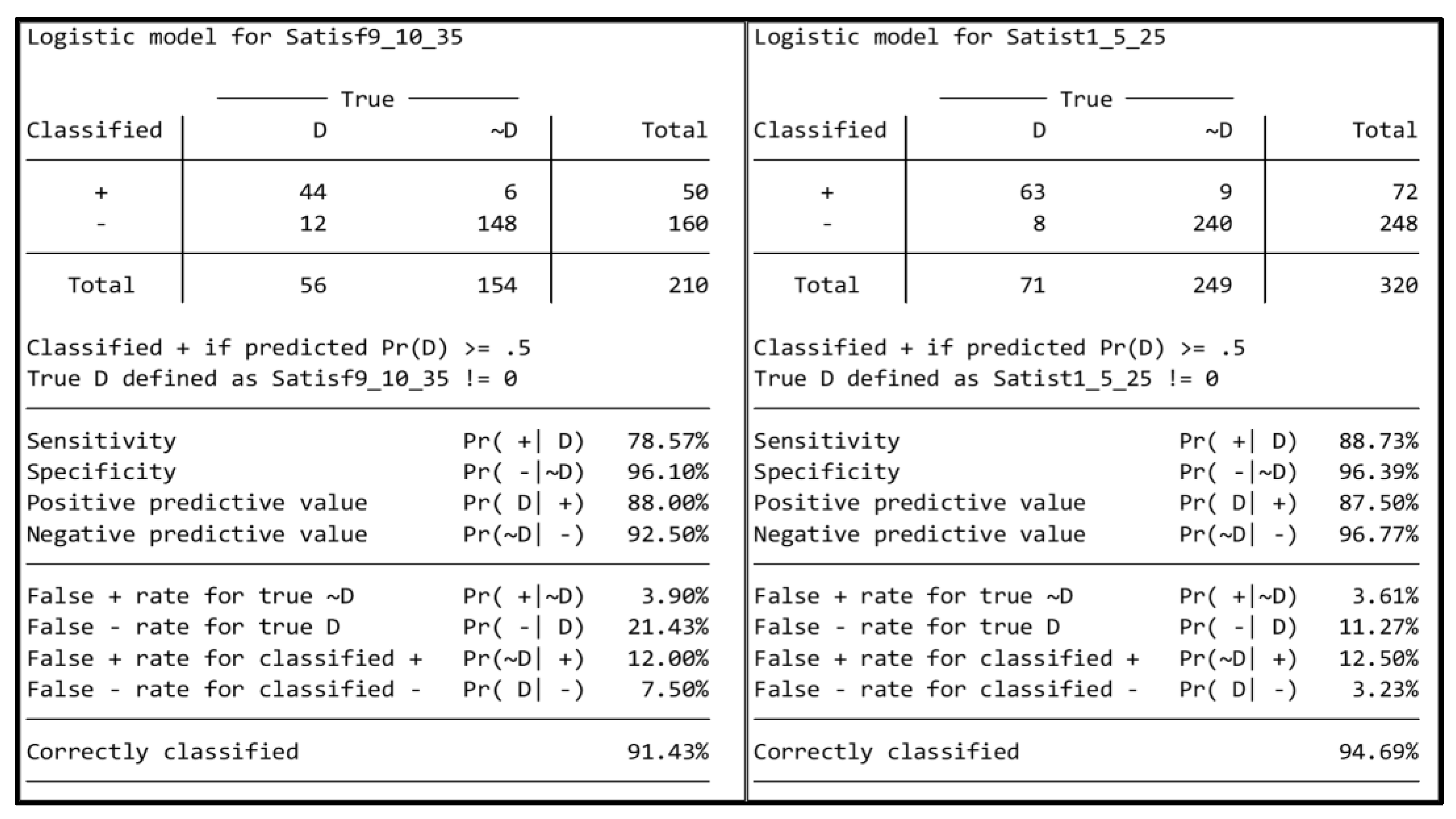
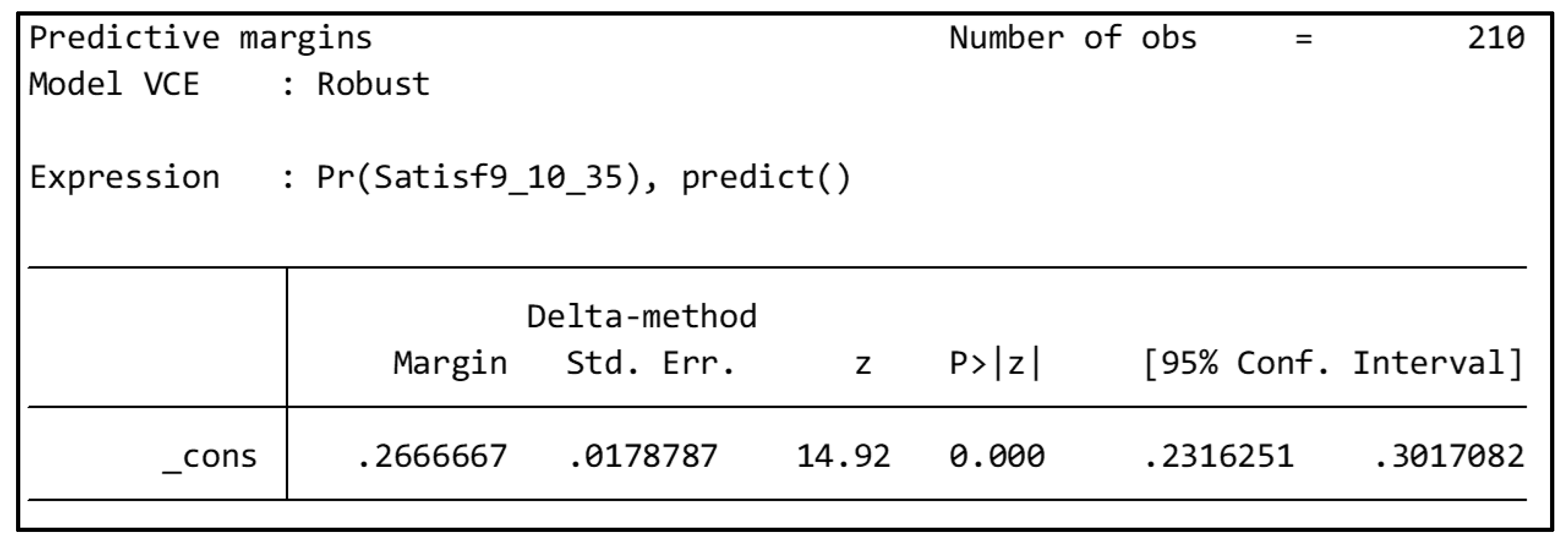
Satisf9_10_35. A dichotomous variable that takes a value of 0 when the condition is not met that more than 35% of its citizens have a satisfaction level equal to or more than 9, and the value of 1 when the condition is met.

(2)

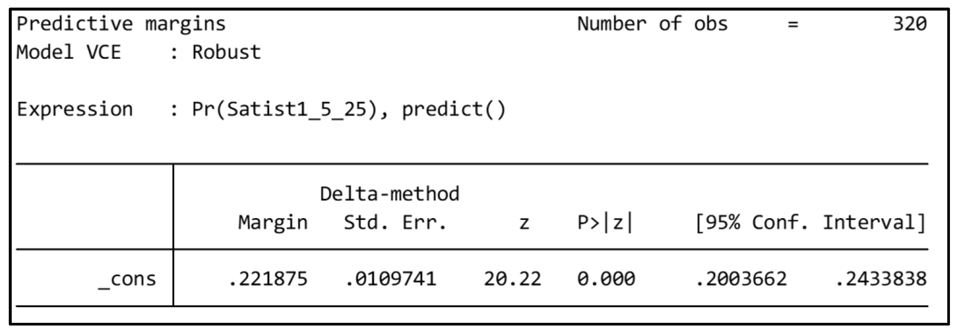
Satist1_5_25. A dichotomous variable with value 0 when the condition is not met that in a country more than 25% of its citizens have a satisfaction level equal to or less than 5, and the value of 1 when the condition is met.

(3)

Satisf8_10. It is a variable that shows the percentage by country of citizens at the level equal to or more than 8.

(4)

Satisf1_5. It is a variable that shows the percentage by country of citizens at the level equal to or less than 5.

The independent and control variables were selected based on a preliminary analysis of all QoL indicators using Eurostat data and macroeconomic indicators such as unemployment (in percentage), GDP per capita, GDP growth (in percentage), life expectancy (years) and the Human Development Index (HDI, in percentage), the Gini index (Gini, in percentage) and the poverty rate at $5.50 dollars per day (Pov55, in percentage). Finally, after reviewing the existing literature and analyzing all these variables and their correlations, those that were highly correlated were eliminated or replaced by others with similar characteristics. In addition, robust models have been built to control the observed heterogeneity. Therefore, the variables selected have been:

• Ageing QoL indicators
  • q_mlc_mh65. Total population living in a dwelling with a leaking roof, damp walls, floors or foundation, or rot. (65 years or over). Percentage.
  • q_safe_da65. Arrears (mortgage or rent, utility bills or hire purchase) from 2003 onwards—EU-SILC survey [ilc_mdes05]. One adult 65 years or over. Percentage.
  • q_hlt_spvg65. Self-perceived health as very good (65 years or over). Percentage.
  • logq_mlc_i65. Logarithm of median equivalised net income (65 years or over). Euro.
• Gender QoL indicator
  • q_gov_dgg. Gender employment gap.
• Environment QoL indicator
  • q_env_pol2.5. Exposure to air pollution by particulate matter. Particulates < 2.5 µm.
  • q_env_polpa. Pollution, grime or other environmental problems. Above 60% of median equivalised income (% Total).
  • q_env_polna. Noise from neighbours or from the street. Above 60% of median equivalised income.
• Other QoL indicators
  • q_act_qlt. Temporary employees. From 15 to 64 years (percentage of employees).
  • q_act_qtl. Long-term unemployment. From 15 to 74 years (percentage of active population).
  • logq_mlc_c. Logarithm of main GDP aggregates per capita. Actual individual consumption. Euro.
• Macroeconomic indicators
  • Gini. Gini Index.
  • Pov55. Poverty headcount ratio at $5.50 a day (2011 PPP) (% of the population).
  • UnEmpl. Unemployment (as a percentage).

The model may be specified as

$$\begin{gathered} L{S}_{it}={\beta }_0+{\displaystyle \sum }_{l=1,\dots ,e}{\beta }_{l}Agein{g}_{it}+{\displaystyle \sum }_{l=e+1,f}{\beta }_{l}Gende{r}_{it}+{\displaystyle \sum }_{l=f+1,\dots ,j}{\beta }_{l}En{v}_{it} \\ \hspace{1em}\hspace{1em}\hspace{1em}\hspace{1em}\hspace{1em}\hspace{1em}\hspace{1em}\hspace{1em}\hspace{1em}\hspace{1em}\hspace{1em}+{\displaystyle \sum }_{l=j+1\dots ,i}{\beta }_{l}Qo{L}_{it}+{\displaystyle \sum }_{l=i+1,\dots ,m}{\beta }_{l}MA{C}_{it}+I\left(WAV{E}_t\right){\beta }_{m+2}+{\epsilon }_{it} \end{gathered}$$

(1)

Our dependent variable LS is “satisfaction with the life”, measured per country “i” how satisfied their citizens are with their lives at WVS wave “t”. We include five vectors whose variables have been mentioned previously. Ageing, gender and env are independent variables, QoL and macroeconomic are control variables. We also wave “t” fixed effects I (WAVE_t) and cluster standard errors at the country level.

Results were achieved using different models as the dependent variable was processed in four ways: two dichotomous variables, one shows the percentage by country of citizens at the level equal to or more than eight and other shows the percentage by country of citizens at the level equal to or less than 5. For dichotomous dependent variables Satisf9_10_35 (models 1) and Satisf1_5_25 (models 2), we used logit models [54,55,56]. For model 3 we used Satisf8_10 as the percentage of citizens whose satisfaction with life was equal to or greater than 8, and in model 4 Satisf1_5 as the percentages of citizens whose satisfaction with life was equal to or less than 5. These two models were performed by linear regression. The same control variables were used to build the models; those that best adapted for models 1 and 3 were selected while the same procedure was applied for models 2 and 4. All models used the same fixed effects as described above.

3. Results

We built two robust models with dummy variables to control wave t fixed effects in vectors and I (WAVEt). Results for models 1 and 2 (logit) and 3 and 4 (OLS) are listed in

Table 1. Logit and Linear Regression Model.

Satisfaction Life	Modelo (1) Logit	Modelo (2) Logit	Modelo (3) Linear Regression	Modelo (4) Linear Regression
Variables	Satisf9_10_35	Satist1_5_25	Satisf8_10	Satisf1_5
q_mlc_mh65		0.0747		0.100 *
		(0.0641)		(0.0519)
q_safe_da65		0.279 ***		0.571 ***
		(0.0598)		(0.126)
q_hlt_spvg65	−0.163 **		0.0263
	(0.0641)		(0.131)
logq_mlc_i65	3.889 ***		10.64 ***
	(0.890)		(1.328)
q_gov_dgg	−0.227 ***	−0.141 ***	−0.123	−0.266 ***
	(0.0692)	(0.0441)	(0.135)	(0.0592)
q_env_pol2.5	0.166 ***		0.115
	(0.0491)		(0.124)
q_env_polpa	−0.619 ***	0.310 ***	−0.561 ***	0.214 **
	(0.235)	(0.0712)	(0.175)	(0.104)
q_env_polna	−0.0191	−0.358 ***	0.0689	0.0588
	(0.0845)	(0.0868)	(0.145)	(0.114)
q_act_qlt	−0.0719	−0.0913 *	0.272 ***	−0.361 ***
	(0.0482)	(0.0471)	(0.0866)	(0.0588)
q_act_qtl	−0.437 **		−1.826 ***
	(0.217)		(0.287)
logq_mlc_c		−5.405 ***		−16.48 ***
		(1.479)		(2.011)
Gini	−0.191 *	0.519 ***	−0.924 ***	0.421 ***
	(0.107)	(0.112)	(0.163)	(0.122)
Pov55	0.603 ***	−0.0666	0.951 ***	−0.588 ***
	(0.109)	(0.101)	(0.143)	(0.193)
UnEmpl		0.0764		0.535 ***
		(0.0908)		(0.203)
3.wave	−3.430 ***	−1.688 **	−2.823 *	1.211
	(0.934)	(0.809)	(1.532)	(0.963)
4.wave	−0.711	−5.276 ***	0.624	0.459
	(0.826)	(1.126)	(1.421)	(0.941)
Constant	−21.36 **	35.58 ***	−9.217	162.5 ***
	(8.407)	(12.11)	(14.19)	(19.73)
Observations	210	320	211	317
R-squared			0.779	0.734
Pseudo R2	0.6034	0.7567

Robust standard errors in parentheses,*** p < 0.01, ** p < 0.05, * p < 0.1.

, and models 1 and 2 marginal effects are listed in

Table 2. Margins y Odds Ratios.

Variables	dx/dy	dx/dy	Odds Ratio	Odds Ratio
	Satisf9_10_35	Satist1_5_25	Satisf9_10_35	Satist1_5_25
q_mlc_mh65		0.0028191		1.077507
q_safe_da65		0.0105275 ***		1.321502 ***
q_hlt_spvg65	−0.0115144 **		0.8494863 **
logq_mlc_i65	0.2745012 ***		48.85412 ***
q_gov_dgg	−0.015995 ***	−0.0053183 ***	0.7972397 ***	0.8686387 ***
q_env_pol2.5	0.0117133 ***		1.180504 ***
q_env_polpa	−0.0437032 ***	0.011691 ***	0.5384075 ***	1.362849 ***
q_env_polna	−0.0013499	−0.013538 ***	0.9810579	0.6987339 ***
q_act_qlt	−0.0050754	−0.0034484 *	0.9306211	0.9127323 *
q_act_qtl	−0.0308778 **		0.6456845 **
logq_mlc_c		−0.2040985 ***		0.0044962 ***
Gini	−0.0135146 *	0.0196163 ***	0.8257518 *	1.681083 ***
Pov55	0.0425479 ***	−0.0025136	1.827178 ***	0.9356063
UnEmpl		0.0028862		1.079423

*** p < 0.01, ** p < 0.05, * p < 0.1.

.

Model 1 has treated the dependent variable as a dichotomous variable with the value of 0 when is not met that more than 35% of its citizens have a satisfaction level equal to or more than nine and the value 1 of when the condition is met. A robust logit model has been constructed with the aforementioned independent variables and has a correct classification of 91.43% (78.57% sensitivity and 96.10% specificity) (Figure 1).

Results show a positive significance (p < 0.01) and consequently an increase in the probability of that in a country more than 35% of its citizens have a satisfaction level equal to or more than 9 with the increase of net income equivalent at 65 years or over (logq_mlc_i65); exposure to air pollution by particulate < 2.5 µm (q_env_pol2.5); poverty index (Pov55).

Results further show an inverse significance at p < 0.01 with variables for gender employment gap (q_gov_dgg), pollution, grime or other environmental problems (q_env_polpa) and time period covered by variables 3wave and with lower significance and effect p < 0.05 with variables for self-perceived health as “very good” at 65 years or over (q_hlt_spvg65) and long-term unemployment (q_act_qtl).

The study of the marginal effect on model 1 shows how the probability that more than 35% of its citizens have a satisfaction level equal to or more than 9 changes if the independent variables change in one unit. This positive effect is more powerful for net income equivalent at 65 years or over (0.2745 ***) and inverse or negative for grime or other environmental problems (−0.0437 ***). Overall, the marginal effect in model 1 is significant, positive and shows a result of 0.27 points; consequently, the probability that in a country more than 35% of its citizens have a satisfaction level equal to, or more than 9 when all variables are average is 26.66%, with a confidence of 95% that the probability is between 23.16% and 30.17% (Figure 2).

Model 2 has treated the dependent variable as a dichotomous variable with value 0 when the condition is not met that in a country more than 25% of its citizens have a satisfaction level equal to or less than 5, and the value of 1 when the condition is met. A robust logit model has been constructed with the aforementioned independent variables and has a correct classification of 94.69% (88.73% sensitivity and 96.39% specificity) (Figure 1).

Results show a positive significance (p < 0.01) and, consequently, an increase in the probability that in a country more than 25% of its citizens have a satisfaction level equal to or less than 5 with the increase of arrears (on mortgage or rent, utility bills or hire purchase) at 65 years or over (q_safe_da65); pollution, grime or other environmental problems (q_env_polpa); Gini index (Gini).

Results further show an inverse significance at p < 0.01 with variables for gender employment gap (q_gov_dgg), noise from neighbours or from the street (q_env_polna), of actual individual consumption (logq_mlc_c) and time period covered by variables 4wave and with lower significance and effect p < 0.05 with time period covered by variables 3wave.

The study of the marginal effect on model 2 shows how the probability that more than 25% of its citizens have a satisfaction level equal to or less than 5 changes if the independent variables change in one unit. This effect is stronger in positive Gini index (0.0196 ***) and inverse or negative on actual individual consumption (−0.2041 ***) Overall, the marginal effect in model 2 is significant, positive and shows a result of 0.22 points; subsequently, the probability that in a country more than 25% of its citizens have a satisfaction level equal to or less than 5 when all variables are average is 22.18%, with a confidence of 95% that the probability is between 20.04% and 24.34% (Figure 3).

Model 3 was performed as an ordinary least squares (OSL) regression with the dependent variable that shows the percentage by country of citizens equal to or more than 8 of LS. The results of this model showed a positive significance at p < 0.01 and consequently an increase in the percentage by country of citizens at the level equal to or more than 8 of LS with an increase of net income equivalent at 65 years or over (logq_mlc_i65); temporary employees (q_act_qlt) and poverty index (Pov55). Results further show an inverse significance at p < 0.01 with pollution, grime or other environmental problems (q_env_polpa); long-term unemployment (q_act_qtl) and Gini index (Gini). The biggest effects on the linear model of life satisfaction with one-unit variations in independent variables are found as positive for net income equivalent at 65 years or over (10.64 ***) and negative for long-term unemployment (−1.826 ***).

Model 4 was performed as an ordinary least squares (OSL) regression with the dependent variable that shows the percentage by country of citizens equal to or less than 5 of LS. The results of this model showed a positive significance at p < 0.01 and therefore, an increase in the percentage by country of citizens at the level equal to or less than 5 of LS with an increase of arrears (on mortgage or rent, utility bills or hire purchase) at 65 years or over (q_safe_da65); pollution, grime or other environmental problems (q_env_polpa); Gini index (Gini) and unemployment (UnEmpl).

Results further show an inverse significance at p < 0.01 with gender employment gap (q_gov_dgg), temporary employees (q_act_qlt); actual individual consumption (logq_mlc_c) and poverty index (Pov55). The biggest effects on the linear model of life satisfaction with one-unit variations in independent variables are found as positive for increase of arrears (on mortgage or rent, utility bills or hire purchase) at 65 years or over (0.571 ***) and negative for actual individual consumption (−16.48 ***).

4. Discussion

In relation to ageing, the income and arrears (mortgage or rent, utility bills or hire purchase) variables stand out. The study shows a positive significance (p < 0.01) of net income equivalent to 65 years and over (in logarithmic) and life satisfaction in models 1 and 3 (analyse high levels of life satisfaction). Thus, an increase of net income equivalent at 65 years or over (in logarithmic), leads to a rise in the probability that 35% of its citizens have a satisfaction level equal to or more than 9 with a probability of 27.45% (model 1), and also increases the percentage per country of citizens with a level of satisfaction level equal to or higher than 8 with β = 10.64 (model 3). These results are in line with studies by [7,10]. In the reverse direction, the individual consumption (the individual consumption variable has been used as income variables to better fit the model) shows significant inverse relationships (p < 0.01)in models 2 and 4 (analyse low levels of life satisfaction). This indicates that as consumption decreases, the probability increases in that more than 25% of a country’s citizens have satisfaction levels equal to or below 5 (model 2), and that the percentage of people in a country with satisfaction levels between 0 and 5 increases (model 4).

Moreover, the results show a relation positive significative (p < 0.01) between arrears (mortgage or rent, utility bills or hire purchase) to adults 65 years or over and low levels of life satisfaction (models 2 and 4). Therefore, a rise in arrears increases the probability that more than 25% of a country’s citizens have satisfaction levels equal to or below 5 (model 2) and increases the percentage of people in a country with satisfaction levels between 0 and 5 (model 4). These results are in line with [39,40] studies. In addition, in the results of model 1, self-perceived health as “very good” to adults 65 years or over variable, appear with a relation negative significative p < 0.05. This indicates that as this variable decreases the probability increases that more than 35% of a country’s citizens have a level equal to or more than 9. These results are in line with the study of [33].

The analysis of the gender employment gap and well-being represented in our work with the variable satisfaction with life confirms that the gender employment gap negatively affects women’s well-being [23]. Model 1 shows an inverse relationship between this variable and LS. Therefore, an increase of the gender employment gap leads to increase in the probability that 35% of the citizens in a country have a satisfaction level equal to or more than 9 with a probability of 1.6% (model 1). Although, the results of models 2 and 4 differ from the above because they present a relation negative significative (p < 0.01) since they are models with low levels of LS. This indicates that as the gender employment gap decreases, the probability increases that more than 25% of a country’s citizens have satisfaction levels equal to or below 5 (model 2), and points out that the percentage of people in a country with satisfaction levels between 0 and 5 increases (model 4). The gender gap results of models 2 and 4 are not in accordance with other studies [23]. It would be interesting to delve into the analysis of gender variables.

Regarding the environmental variables analysed, this study shows a relation negative significative effect p < 0.01 of pollution, grime or other environmental problems with life satisfaction in models with high satisfaction levels (models 1 and 3), and the inverse sense in models with low satisfaction (models 2 and 4). This is in line with the study of [46,57]. However, the exposure to air pollution by particulate < 2.5 µm presents a relation positive significative in model 1. Concerning the relationship between the noise from neighbours or from the street variable and LS, the model 2 results show a relation inverse significative p < 0.01. Therefore, its decrease increases the probability that more than 25% of a country’s citizens have satisfaction levels equal to or below 5. In line with the study conducted by [58], and in the opposite direction to the results of this work, are the studies by [59,60,61].

Concerning the variables of employment, this study shows a positive significative effect p < 0.01 of the percentage of the temporary employees (15 to 64 years) with LS in model 3, and inverse in model 4. Those results are in the same line as the studies by [15]. However, unemployment indicators show different behaviours depending on the duration of this situation. Our research shows how unemployment, in general, maintains a positive relationship in model 4 (model with low satisfaction 1–5). Its increase raises the percentage of people in a country with satisfaction levels between 0 and 5 (model 4). With respect to long-term unemployment, the results show a negative significative p < 0.05 in model 1 and p < 0.01 in model 3. Accordingly, a decrease of long-term unemployment leads to an increase in the probability that 35% of its citizens have a satisfaction level equal to or more than 9 (model 1), and also increases the percentage per country of citizens with a level of satisfaction equal to or higher than 8 (model 3). The results are similar to the study carried out by [16,17,18].

Relating the inequality (Gini variable), the results show a relation positive significative p < 0.01 in models 2 and 4, and negative in model 3. Therefore, the increase in inequality increases the probability that more than 25% of a country’s citizens have satisfaction levels equal to or below 5 (model 2) and that the percentage of people in a country with satisfaction levels between 0 and 5 increases (model 4). In addition, its decrease increases the percentage per country of citizens with a satisfaction level equal to or higher than 8 (model 3). These results are in line with the study by [62].

Furthermore, the analysis shows that the poverty indicator in a country (Pov55) shows a significant positive relationship p < 0.01 in models 1 and 3, with a marginal effect in model 1 (4.25%) and in model 3 (0.951). It also shows an inverse relationship with the percentage per country of citizens at or below level 5 (model 4), but it is not significant in model 2. These results differ from the study conducted by [62,63] and open the debate about poverty and its effects on citizens in a developed country.

5. Conclusions

To conclude, it is possible to affirm from these results that countries with a higher percentage of the population aged 65 and over who have arrears (mortgage or rent, utility bills or hire purchase) present a higher percentage of citizens with low levels of LS (1–5). Therefore, hypothesis 1 is accepted.

We can also point out that as the income of people aged 65 and over increases, the percentage of people with life satisfaction levels equal to or higher than 8 increases (hypothesis 2 is accepted), and raises the probability that a country will have more than 35% of its population at satisfaction levels 9 and 10. In addition, as the percentage of the population aged 65 and over who perceive their health as “very good” increases, the probability of a country having more than 35% of its population in satisfaction levels 9 and 10 increases too, but with a lower significance p < 0.05. Consequently, hypothesis 3 is accepted considering its lower significance.

This paper also shows a significant inverse relationship p < 0.01 between the gender labour gap and LS indicators in three models (models 1, 2 and 4). Model 1 is in line with previous studies, but models 2 and 3 should be studied in more depth and detail as they show that as the gender employment gap decreases, this increases the probability that more than 25% of a country’s citizens have satisfaction levels equal to or below 5 (model 2) (Hypothesis 4 is rejected), and indicates that the percentage of people in a country with satisfaction levels between 0 and 5 increases (model 4).

With regard to the analysis of the environmental variables, specifically the variable pollution, grime, or other environmental problems, the study reveals an inverse relationship between this indicator and life satisfaction in the models with high levels of satisfaction (model 1 and 3) and a positive relationship in models 2 and 4. These results are in line with previous studies and lead to the acceptance of hypothesis 5.

Finally, it is important to note the significant positive relationship of inequality (Gini index) with the models that represent low levels of satisfaction with life. These results go in the same direction as other studies analysed. Unlike this, the poverty indicator shows a relationship contrary to the expected one that should be studied further. What is more, we believe that it would be interesting to study these variables, including developing and underdeveloped countries in the study.

References

1. D’Acci, L. Measuring Well-Being and Progress. Soc. Indic. Res. 2010, 104, 47–65. [Google Scholar] [CrossRef] [Green Version]
2. Rogers, D.S.; Duraiappah, A.K.; Antons, D.C.; Munoz, P.; Bai, X.; Fragkias, M.; Gutscher, H. A vision for human well-being: Transition to social sustainability. Curr. Opin. Environ. Sustain. 2012, 4, 61–73. [Google Scholar] [CrossRef]
3. Benjamin, D.J.; Heffetz, O.; Kimball, M.S.; Szembrot, N. Beyond Happiness and Satisfaction: Toward Well-Being Indices Based on Stated Preference. Am. Econ. Rev. 2014, 104, 2698–2735. [Google Scholar] [CrossRef] [Green Version]
4. Diener, E.; Lucas, R.; Schimmack, U.; Helliwell, J. Well-Being for Public Policy; Oxford University Press: Oxford, UK, 2009. [Google Scholar]
5. Brooks, J.S. Avoiding the Limits to Growth: Gross National Happiness in Bhutan as a Model for Sustainable Development. Sustainability 2013, 5, 3640–3664. [Google Scholar] [CrossRef] [Green Version]
6. Li, Y.; Guan, D.; Tao, S.; Wang, X.; He, K. A review of air pollution impact on subjective well-being: Survey versus visual psychophysics. J. Clean. Prod. 2018, 184, 959–968. [Google Scholar] [CrossRef]
7. Cortés, S.G.; Delgado, R.M.J.; Ortega, G.M. La medición de la felicidad y la construcción de indicadores de bienestar subjetivo. Aplicación del modelo de Rasch. In Claves Para un Desarrollo Sostenible la Creatividad y Hapiness Ma-Nagement Como Portafolio de la Innovación Tecnológica, Empresarial y Marketing Social; Rafael Ravina Ripoll, Luis Bayardo Tobar Pesántez, Araceli Galiano Coronil Coords: Granada, Spain, 2018; pp. 81–98. ISBN 978-84-9045-679-8. [Google Scholar]
8. Stiglitz, J.; Sen, A.; Fitoussi, J.P. The Measurement of Economic Performance and Social Progress Revisited. Reflections and Overview; Commission on the Measurement of Economic Performance and Social Progress: Paris, France, 2009. [Google Scholar]
9. Pavot, W.; Diener, E. Review of the Satisfaction With Life Scale. In Assessing Well-Being; Diener, E., Ed.; Springer: Dordrecht, The Netherlands, 2009; Volume 39, pp. 101–117. [Google Scholar] [CrossRef]
10. Stutzer, A. The role of income aspirations in individual happiness. J. Econ. Behav. Organ. 2004, 54, 89–109. [Google Scholar] [CrossRef] [Green Version]
11. Sweeney, P.D.; McFarlin, D.B.; Inderrieden, E.J. Research notes. Using relative deprivation theory to explain satisfaction with income and pay level: A multistudy examination. Acad. Manag. J. 1990, 33, 423–436. [Google Scholar] [CrossRef]
12. Layard, R. Happiness: Has Social Science a Clue? London School of Economics: London, UK, 2003; Volume 24. [Google Scholar]
13. Jahoda, M. Empleo y Desempleo: Un Análisis Socio-Psicológico; Ediciones Morata: Madrid, Spain, 1987; pp. 18–19. [Google Scholar]
14. Ross, C.E.; Van Willigen, M. Education and the Subjective Quality of Life. J. Health Soc. Behav. 1997, 38, 275–297. [Google Scholar] [CrossRef]
15. Dawson, C.; Veliziotis, M.; Hopkins, B. Temporary employment, job satisfaction and subjective well-being. Econ. Ind. Democr. 2014, 38, 69–98. [Google Scholar] [CrossRef] [Green Version]
16. Vansteenkiste, M.; Lens, W.; De Witte, S.; De Witte, H.; Deci, E.L. The‘why’ and‘why not’ of job search behaviour: Their relation to searching, unemployment experience, and well-being. Eur. J. Soc. Psychol. 2004, 34, 345–363. [Google Scholar] [CrossRef]
17. Binder, M.; Coad, A. Heterogeneity in the Relationship Between Unemployment and Subjective Wellbeing: A Quantile Approach. Economica 2015, 82, 865–891. [Google Scholar] [CrossRef] [Green Version]
18. Lucas, R.E.; Clark, A.E.; Georgellis, Y.; Diener, E. Unemployment Alters the Set Point for Life Satisfaction. Psychol. Sci. 2004, 15, 8–13. [Google Scholar] [CrossRef] [PubMed] [Green Version]
19. Clark, A.; Knabe, A.; Rätzel, S. Boon or bane? Others’ unemployment, well-being and job insecurity. Labour Econ. 2010, 17, 52–61. [Google Scholar] [CrossRef] [Green Version]
20. Klasen, S. Gender-related Indicators of Well-being. In Human Well-Being; Palgrave Macmillan: London, UK, 2007; pp. 167–192. [Google Scholar]
21. Perrons, D. Final Comparative Report: Flexible Working and the Reconciliation of Work and Family Life-or a New form of Precariousness. In Equality between Men and Women. European Commission; Employment and Social Affairs: Brussels, Belgium, 1998. [Google Scholar]
22. Figart, D.M.; Mutari, E. Horarios largos y cortos: Qué puede aprender norteamérica de europa? Investig. Econ. 2000, 60, 53–71. [Google Scholar]
23. Offer, S.; Schneider, B. Revisiting the gender gap in time-use patterns: Multitasking and well-being among mothers and fathers in dual-earner families. Am. Sociol. Rev. 2011, 76, 809–833. [Google Scholar] [CrossRef]
24. Hetschko, C.; Knabe, A.; Schöb, R. Changing Identity: Retiring from Unemployment. Econ. J. 2014, 124, 149–166. [Google Scholar] [CrossRef] [Green Version]
25. Ponomarenko, V.; Leist, A.K.; Chauvel, L. Increases in well-being in the transition to retirement for the unemployed: Catching up with formerly employed persons. Ageing Soc. 2019, 39, 254–276. [Google Scholar] [CrossRef]
26. Flint, E.; Bartley, M.; Shelton, N.; Sacker, A. Do labour market status transitions predict changes in psychological well-being? J. Epidemiol. Community Health 2013, 67, 796–802. [Google Scholar] [CrossRef] [PubMed]
27. LaMontagne, A.D.; Milner, A.; Krnjacki, L.; Schlichthorst, M.; Kavanagh, A.; Page, K.; Pirkis, J. Psychosocial job quality, mental health, and subjective well-being: A cross-sectional analysis of the baseline wave of the Australian longitudinal study on male health. BMC Public Health 2016, 16, 33–41. [Google Scholar] [CrossRef] [Green Version]
28. Marans, R.W. Understanding environmental quality through quality of life studies: The 2001 DAS and its use of subjective and objective indicators. Landsc. Urban Plan. 2003, 65, 73–83. [Google Scholar] [CrossRef]
29. Steptoe, A.; Deaton, A. A Stone, A. Subjective wellbeing, health, and ageing. Lancet 2015, 385, 640–648. [Google Scholar] [CrossRef] [Green Version]
30. Rétsági, E.; Prémusz, V.; Makai, A.; Melczer, C.; Betlehem, J.; Lampek, K.; Ács, P.; Hock, M. Association with subjective measured physical activity (GPAQ) and quality of life (WHOQoL-BREF) of ageing adults in Hungary, a cross-sectional study. BMC Public Health 2020, 20, 1–11. [Google Scholar] [CrossRef] [PubMed]
31. Michalos, A.C.; Zumbo, B.D. Healthy Days, Health Satisfaction and Satisfaction with the Overall Quality of Life. Soc. Indic. Res. 2002, 59, 321–338. [Google Scholar] [CrossRef]
32. Hsieh, C.-M. The Relative Importance of Health. Soc. Indic. Res. 2008, 87, 127–137. [Google Scholar] [CrossRef]
33. Ayala, L.; José, M. Labeaga & Carolina Navarro, “undated”. “Housing deprivation and health status: Evidence from Spain?”. In Working Papers; Fedea: Madrid, Spain, 2005; p. 02. [Google Scholar]
34. Bowling, A.; Windsor, J. Towards the Good Life: A Population Survey of Dimensions of Quality of Life. J. Happiness Stud. 2001, 2, 55–82. [Google Scholar] [CrossRef]
35. Skevington, S.M. Qualities of life, educational level and human development: An international investigation of health. Soc. Psychiatry Psychiatr. Epidemiol. 2009, 45, 999–1009. [Google Scholar] [CrossRef] [PubMed] [Green Version]
36. Chen, C. Aging and Life Satisfaction. Soc. Indic. Res. 2001, 54, 57–79. [Google Scholar] [CrossRef]
37. Abbasimoghadam, M.A.; Dabiran, S.; Safdari, R.; Djafarian, K. Quality of life and its relation to sociodemographic factors among elderly people living in Tehran. Geriatr. Gerontol. Int. 2009, 9, 270–275. [Google Scholar] [CrossRef]
38. Addae-Dapaah, K.; Juan, Q.S. Life Satisfaction among Elderly Households in Public Rental Housing in Singapore. Health. 2014, 6, 1057–1076. [Google Scholar] [CrossRef] [Green Version]
39. Gerlach-Kristen, P.; Lyons, S. Determinants of mortgage arrears in Europe: Evidence from household microdata. Int. J. Hous. Policy 2017, 18, 545–567. [Google Scholar] [CrossRef]
40. Białowolski, P. Hard Times! How do Households Cope with Financial Difficulties? Evidence from the Swiss Household Panel. Soc. Indic. Res. 2017, 139, 147–161. [Google Scholar] [CrossRef]
41. Powdthavee, N. Unhappiness and Crime: Evidence from South Africa. Economica 2005, 72, 531–547. [Google Scholar] [CrossRef] [Green Version]
42. Staubli, S.; Killias, M.; Frey, B.S. Happiness and victimisation: An empirical study for Switzerland. Eur. J. Criminol. 2014, 11, 57–72. [Google Scholar] [CrossRef]
43. Spencer, N.; Liu, Z. Victimisation and life satisfaction: Evidence from a high crime country. Soc. Indic. Res. 2019, 144, 475–495. [Google Scholar] [CrossRef]
44. Møller, V. Resilient or Resigned? Criminal Victimisation and Quality of Life in South Africa. Soc. Indic. Res. 2005, 72, 263–317. [Google Scholar] [CrossRef]
45. Cooper, C.D.; Alley, F.C. Air Pollution Control: A design Approach; Waveland Press: Long Grove, IL, USA, 2010. [Google Scholar]
46. Welsch, H. Environment and happiness: Valuation of air pollution using life satisfaction data. Ecol. Econ. 2006, 58, 801–813. [Google Scholar] [CrossRef]
47. Giovanis, E. Worthy to lose some money for better air quality: Applications of Bayesian networks on the causal effect of income and air pollution on life satisfaction in Switzerland. Empir. Econ. 2018, 57, 1579–1611. [Google Scholar] [CrossRef] [Green Version]
48. Orru, K.; Orru, H.; Maasikmets, M.; Hendrikson, R.; Ainsaar, M. Well-being and environmental quality: Does pollution affect life satisfaction? Qual. Life Res. 2016, 25, 699–705. [Google Scholar] [CrossRef] [PubMed]
49. Manning, C.; Clayton, S. Threats to mental health and well-being associated with climate change. In Psychology and Climate Change; Academic Press: Cambridge, MA, USA, 2018; pp. 217–244. [Google Scholar]
50. Systems Institute; WVSA Secretariat. In World Values Survey: All Rounds—Country-Pooled Datafile; Inglehart, R.; Haerpfer, C.; Moreno, A.; Welzel, C.; Kizilova, K.; Diez-Medrano, J.; Lagos, M.; Norris, P.; Ponarin, E.; Puranen, B.; et al. (Eds.) Systems Institute & WVSA Secretariat: Madrid, Spain, 2020; Available online: http://www.worldvaluessurvey.org/WVSDocumentationWVL.jsp (accessed on 15 February 2021).
51. European Values Study. Integrated Dataset (EVS 2017). In ZA7500 Data File Version 4.0; GESIS Data Archive: Cologne, Germany, 2017. [Google Scholar] [CrossRef]
52. Blanchflower, D.G.; Oswald, A.J. International Happiness: A New View on the Measure of Performance. Acad. Manag. Perspect. 2011, 25, 6–22. [Google Scholar] [CrossRef] [Green Version]
53. Letelier-S, L.E.; Sáez-Lozano, J.L. Expenditure Decentralization: Does It Make Us Happier? An Empirical Analysis Using a Panel of Countries. Sustainability 2020, 12, 7236. [Google Scholar] [CrossRef]
54. Aldrich, J.; Nelson, F. Quantitative Applications in the Social Sciences: Linear Probability, Logit, and Probit Models; SAGE Publications, Inc.: Thousand Oaks, CA, USA, 1984. [Google Scholar]
55. Hosmer, D.W.; Lemeshow, S. Applied Logistic Regression; John Wiley & Sons: New York, NY, USA, 2000. [Google Scholar]
56. Cramer, J.S. Logit Models from Economics and Other Fields; Cambridge University Press: Cambridge, UK, 2003. [Google Scholar] [CrossRef] [Green Version]
57. Luechinger, S. Life satisfaction and transboundary air pollution. Econ. Lett. 2010, 107, 4–6. [Google Scholar] [CrossRef]
58. Ortega-Gil, M.; Cortés-Sierra, G.; ElHichou-Ahmed, C. The Effect of Environmental Degradation, Climate Change, and the European Green Deal Tools on Life Satisfaction. Energies 2021, 14, 5839. [Google Scholar] [CrossRef]
59. Clark, C.; Paunovic, K. WHO Environmental Noise Guidelines for the European Region: A Systematic Review on Environmental Noise and Quality of Life, Wellbeing and Mental Health. Int. J. Environ. Res. Public Health 2018, 15, 2400. [Google Scholar] [CrossRef] [PubMed] [Green Version]
60. JarosiŃska, D.; Héroux, M.-È.; Wilkhu, P.; Creswick, J.; Verbeek, J.; Wothge, J.; Paunović, E. Development of the WHO Environmental Noise Guidelines for the European Region: An Introduction. Int. J. Environ. Res. Public Health 2018, 15, 813. [Google Scholar] [CrossRef] [PubMed] [Green Version]
61. Shepherd, D.; Dirks, K.; Welch, D.; McBride, D.; Landon, J. The Covariance between Air Pollution Annoyance and Noise Annoyance, and Its Relationship with Health-Related Quality of Life. Int. J. Environ. Res. Public Health 2016, 13, 792. [Google Scholar] [CrossRef] [PubMed] [Green Version]
62. Cooper, D.; McCausland, W.D.; Theodossiou, I. Income Inequality and Wellbeing: The Plight of the Poor and the Curse of Permanent Inequality. J. Econ. Issues 2013, 47, 939–958. [Google Scholar] [CrossRef]
63. Lawless, N.M.; Lucas, R. Predictors of Regional Well-Being: A County Level Analysis. Soc. Indic. Res. 2010, 101, 341–357. [Google Scholar] [CrossRef]
Figure 1. Classification statistics and table logit models (Models 1 y 2).
Land 10 01314 g001
Figure 2. Predictive Margins Model 1.
Land 10 01314 g002
Figure 3. Predictive Margins Model 2.
Land 10 01314 g003