Research on the Evaluation of Real Estate Inventory Management in China

Abstract

Inventory management not only determines the health of the real estate market development, but also affects the regional economy and the capacity of sustainable social development. In this paper we use the DPSIR framework to integrate multi-dimensional influence factors, such as economic, social, and environmental factors, to construct a real estate inventory management performance evaluation and obstacle diagnosis model, and conduct an empirical study on 31 Chinese provinces and cities. The results show that: first, China’s real estate inventory is huge in size, with significant spatial heterogeneity and agglomeration; second, China’s real estate inventory management performance is unsatisfactory and still shows no improvement despite the strong policy intervention of the central and local governments; third, the obstacle factors of real estate inventory management are becoming increasingly diversified and complicated, with great differences among provinces—significantly, Profits of Real Estate Enterprises, Disposable Income of Urban Residents, Financial Revenue, Per Capital GDP, Resident Population, Gross Domestic Product, Total Retail Sales of Social Consumer Goods, Financial Expense, and Loans Balance of Financial Institutes are critical obstacle factors; and fourth, it is suggested that, on the basis of mastering the actual conditions of supply and demand in the real estate market, differentiated and precise response strategies should be formulated by integrating near-term and long-term goals, direct and indirect forces, and administrative and market instruments.

1. Introduction

1.1. Background

Inventory is an important part of the material security of enterprise production and sales, having a high place in enterprise operations and remaining a hot topic of concern for business managers and researchers [1,2]. A certain amount of inventory helps enterprises ensure normal, continuous, and stable production, and also helps to respond and meet customer needs in a timely manner, maintain a corporate reputation, and consolidate market share. Real estate is a leading industry in most countries of the world, featuring a large investment scale, high product value, high risk, and high return. Against the background of high inventory and high housing prices, the level of inventory management has become an important index reflecting the competition of real estate enterprises, the development of the industry, and the health of market operation, and has a significant impact on the sustainable development of cities and regions, and even the national economy and society. It has received attention from researchers in different disciplines such as land management, spatial planning, human geography, real estate economics, and business management [3].

China’s real estate market is huge in scale, and with the continuous increase in inventory in recent years, financial, market, economic, and social risks continue to accumulate, making it a typical representative in the world [4]. After decades of rapid development, China’s real estate has experienced a decline in investment growth and oversupply in the market. Especially since 2010, China’s real estate market has fallen into the dilemma of an increasing inventory. High inventory and high housing prices have become a great threat to the healthy development of the economy and social harmony and stability. In 2015, the Central Economic Work Conference made real estate “destocking” one of the government’s five key tasks, indicating that real estate destocking has officially risen to a national task. Local governments at all levels have issued special policies on real estate destocking, such as Opinions of Shaanxi Provincial People’s Government’s on Real Estate Destocking and Structure Optimization, Implementation Opinions of Qinghai Provincial People’s Government on Promoting Real Estate Destocking, Implementation Opinions of Anhui Provincial People’s Government on Destocking and Promoting Stable Development of Real Estate Market, Opinions of General Office of Chongqing Municipal People’s Government on Promoting the Stable and Healthy Development of the City’s Commercial and Commercial Real Estate Market, and Opinions of Guangzhou on Further Promoting the Stable and Healthy Development of the City’s Real Estate Market.

The central government and local governments at all levels have successively implemented a number of real estate destocking policies and achieved certain results after years of management, but the achievement has failed to meet expectations and there is still a big gap to fill to reach the ultimate goal [5]. China’s real estate inventory is huge, and there is a significant spatial difference in destocking pressure, making the task of inventory management arduous and complicated. As indicated in the Market Size Report on Global Real Estate, China has grown to be the fourth largest real estate market in the world, with global representation. Therefore, it is of great theoretical significance and practical value to carry out research on the inventory management performance evaluation of China’s real estate market and analyze the main obstacles and coping strategies for destocking.

1.2. Literature Review

Inventory management is a difficult issue of long-term and continuous concern for industry, politics, and academia. The current research focuses on inventory management technology innovation and application, development of inventory management strategies for multiple scenario models, and exploration of specific enterprise and product inventory management methods [6]. It should be noted that real estate inventory management is receiving more and more attention as an emerging field.

1.2.1. Research on Technology Innovation and Application of Inventory Management

The research foci on inventory management technology innovation and application in different fields, industries, and enterprises include inventory management model and system development, method innovation and application, and index and index construction [7]. For example, Yan [8], Melikov [9], Preil [10], and Drakaki [11] developed inventory management models and systems based on System Dynamics, Markov Model, Artificial Intelligence, and Colored Petri Net-based modeling methods. Mamani [12] and Borgonovo [13] conducted a robustness and sensitivity analysis of inventory management models. Hill [14] developed a forecastability quotient index for inventory forecasting. Subramanian [15] developed a supply chain inventory management control model, and Perez [16] proposed an optimization method for inventory management algorithms. Borgonovo [17] developed a new inventory management model sensitivity measure using differential importance (D) and the comparative statics (CS) techniques. Almaktoom [18] developed a method of quantifying the reliability of an inventory management system, and Jonsson [19] conducted a comparative study of different methods of safety inventory management (SIM). Lei [20] analyzed the dynamics of the Nonlinear Inventory Management System by means of the eigenvalue trajectory, bifurcations, chaotic attractor, and yjr the largest Lyapunov exponent diagram, Fractional-Order Approximate Entropy, finding the equilibrium of the inventory management system. Rahaman [21] analyzed the synergy of inventory management in uncertain environments based on memory and learning effects. In general, the existing research focuses on the development technology of models, systems, and algorithms, but pays little attention to the performance evaluation and application effect of inventory management. Technology innovation is a front-end research topic, while technology application and effect evaluation is a back-end research topic. In the enterprise development practice, more emphasis is placed on the latter, as enterprises are eager to know what state and problems of inventory management are when using a certain system or model. However, the existing papers give little attention to inventory management performance evaluation methods and problem diagnosis technology, which does not match the practical needs and restricts the application and reinvention of inventory management technology.

1.2.2. Research on Multi-Scenario Inventory Management Strategies

As a complex, non-linear, and systematic project, inventory management is greatly influenced by various external environment and internal factors, so scholars pay close attention to the research of differentiation strategy of inventory management in different scenarios. For example, Bendavid [22], Steinker [23], and Katehakis [24] argued that the goal of inventory management models is to achieve a continuous balance between costs and sales by effective strategies, and it is necessary to consider the constraints of working capital. Sharma [25] analyzed inventory management models in the context of order constraints; Fu [26] and Buzacott [27] analyzed inventory management methods in inventory-dependent financing scenarios; Herrmann [28] analyzed inventory management models during high-frequency trading in imperfectly competitive environments; Xu [29], Chen [30], and Mokhtari [31] analyzed inventory management technology in the context of joint pricing; Guo [32] studied inventory management schemes under the condition of mass customization; Chen [33], Xiao [34], and Transchel [35] analyzed inventory management strategies under dynamic price effects; Park [36] analyzed optimal inventory management schemes under buy-one-give-one conditions; Xie [37] and Muharremoglu [38] analyzed measures to achieve inventory management robustness in the presence of multiple supply sources; Mascle [39] developed an inventory management system with integrated sales volume forecasting; and Nenes [40] and Cao [41] provide a case study of inventory management in irregular and non-smooth demand scenarios. In summary, to improve the competitiveness and adaptability of enterprises, scholars have analyzed inventory management models in many situations from different perspectives, mainly focusing on case and qualitative studies, with less attention to quantitative and empirical studies, thus impairing the accuracy and practicability of the research conclusions.

1.2.3. Research on Inventory Management of Specific Enterprises and Products

The current research focuses mainly on the inventory management of industrial manufacturing, retail, and supply chain service companies, while the inventory management for special products, such as oil, disaster relief supplies, and shared bicycles, is attracting increasing attention [42]. In the field of industrial production, the focus is placed on spare parts inventory management in the manufacturing industry. For example, Muniz [43] and Turrini [44] analyzed spare parts inventory management in the Brazilian mining industry and German renewable energy industry, Kranenburg [45] analyzed service differentiation of spare parts inventory management, and Dendauw [46] proposed the critical state of spare parts inventory management. Furthermore, remanufactured product inventory management [47], supply chain inventory management in Industry 4.0 [48,49], and industrial inventory management in China [50] and India [51] have also received some attention, and there are many empirical research papers. In the supply chain and services sector, the main focus is on retailer inventory management. Jaksic [52] analyzed optimal inventory management in the context of supply backorders for retailers; Agrawal [53] analyzed optimal inventory management models for retail chain stores in the context of demand differentiation (differences in economic conditions, culture and demographics, and store formats); Ehrenthal [54] analyzed inventory management solutions in different seasonal demand differentiation scenarios; Turgut [55] studied retail inventory management models with back-office effects; Saputro [56], Sarkar [57], and DeCroix [58] analyzed inventory management methods in the context of supply disruptions; and Hasan [59] proposed an inventory management scheme for e-commerce retailers. In the field of special product inventory management, Raviv [60] and Swaszek [61] analyzed inventory management technology for shared bicycles; Chuang [62] analyzed inventory management solutions for General Motors, Mostafaei [63], Siddiqui [64], and Dimas [65] analyzed inventory management strategies for oil; Toyasaki [66], Loree [67], and Natarajan [68] analyzed the inventory management model for humanitarian relief materials; and Paam [69] and Golas [70] analyzed the inventory management methods for agriculture.

1.2.4. Research on Inventory Management in Real Estate Market

Real estate inventory management has been on the rise. Geman [71] was the first to introduce the inventory management concept into the real estate and conducted an empirical study of the UK. Pham [72], based on an analysis of dynamic panel data of Vietnamese real estate companies for the 2011–2018 period, believes that inventory size, installment payment, and financing policies are the main factors affecting sales growth. Bian [73] studied the effect of inventory size on residential prices and liquidity and concluded that real estate inventories bear obvious externality. Caplin [74] constructed a joint model between real estate inventories, prices, and sales, arguing that high inventories lead to higher prices. Ott [75] found high inventories of real estate in the US, particularly in cities such as Atlanta, Las Vegas, and Orlando, and proposed an optimal staging and inventory decision model for large residential developments. Wen [76], based on the real estate practice in China, proposed an inventory management model in the context of demand uncertainty and dynamic price changes. Kwoun [77] introduced system dynamics to analyze unsold new housing stocks, and developed Causal Loop Diagrams and Stock-Flow Diagrams for quantitative simulation. Morales [78], Jiang [79], and Muczynski [80] provided a brief analysis of real estate inventories in Brazil, China, and Poland. Yoo [81] and Nam [82] conducted an in-depth case study of the factors influencing real estate inventories and their management responses in Gyeonggi Province, South Korea. Real estate inventory management research is generally still in its infancy, and the existing research is fragmented significantly, lacking a systematic and mature research framework and methods.

1.3. Aim and Question

The change trends in real estate inventory levels vary across countries and industries, and the factors affecting inventory management are also very different. China is a global representative in real estate inventory management, so the empirical study of China can provide experience and decision-making reference for countries and regions with similar conditions. China’s real estate development is characterized by significant spatial heterogeneity, with uneven destocking pressure in different provincial and municipal governments. To reveal the current status, changing trends, performance levels, major obstacles, and management strategies of China’s real estate inventory, this paper is devoted to answering the following three questions: (1) What are the characteristics of the spatial and temporal evolution of China’s real estate inventory, including the time series change trend and spatial pattern characteristics under different measurement indexes? (2) How does one construct the performance evaluation index system of China’s real estate inventory management, including the index composition, weight scheme, and result grading? (3) What is the optimization strategy for real estate inventory management in China, including the analysis of the influence factors of inventory management, identification of the main obstacle factors, and policy design suggestions?

2. Research Design

2.1. Study Area: China

The study area of this paper covers 31 provinces, autonomous regions, and municipalities directly under the central government of China, excluding Taiwan, Hong Kong, and Macao due to a lack of data (Figure 1). According to the data released by the National Bureau of Statistics, China’s real estate inventory showed a rapid rise in scale in 2010, and a decline only after 2015 under the strong policy intervention. However, it currently is still at a high level. Significantly, the scale of China’s long-term real estate inventory (staying on the market for 3 years or more) has continued to grow rapidly over the same period, with a surge in growth in the last two years in particular (Figure 2). At the same time, from the perspective of population and land scale in the study area, the characteristics of unbalanced development and inequality are prominent, which should be properly considered when studying the spatial differentiation of real estate inventory (Figure 3).

2.2. Research Methods

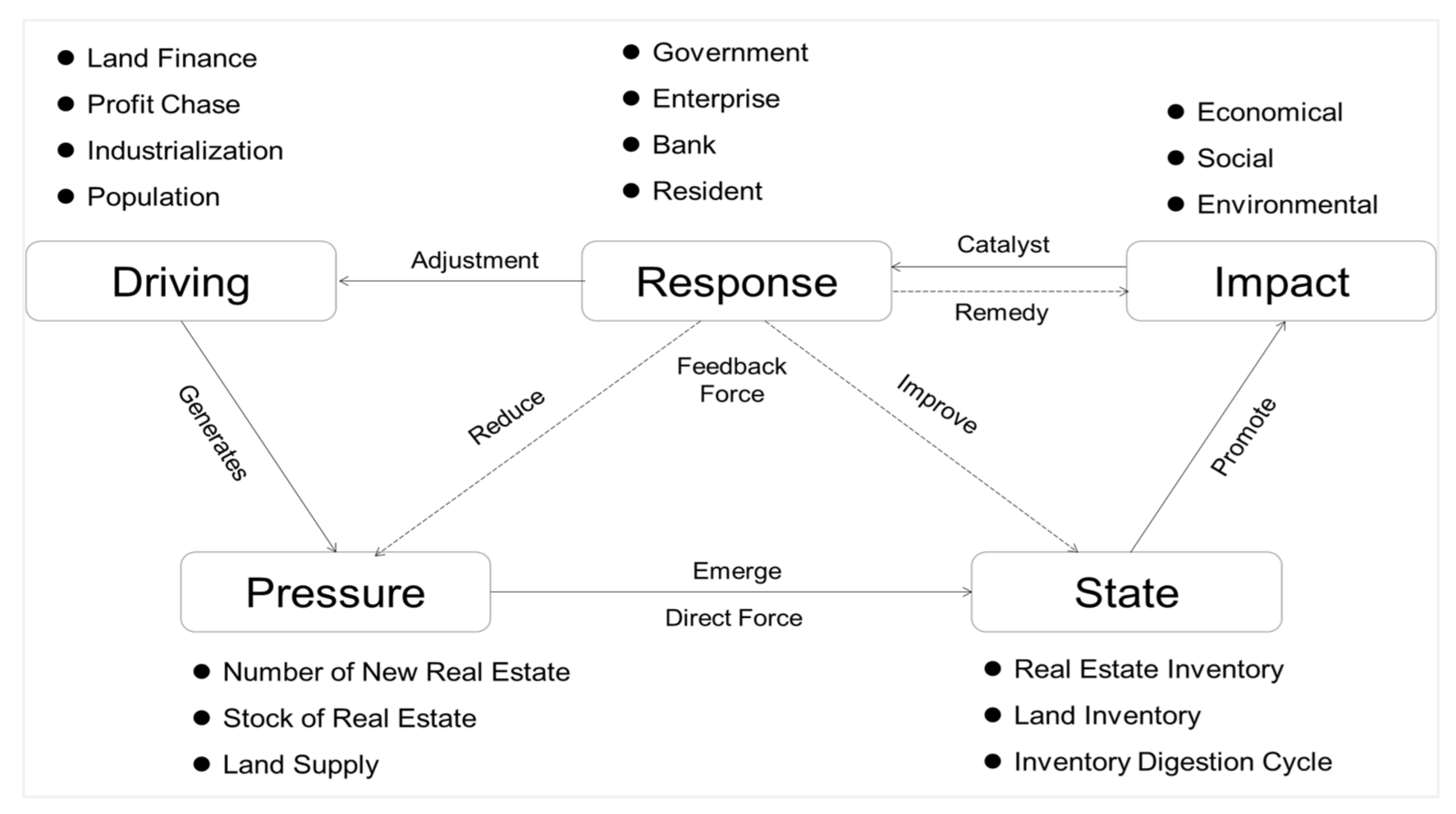
2.2.1. DPSIR Model

The Driver–Pressure–State–Impact–Response (DPSIR) model, created by the European Environment Agency, serves as a comprehensive model dedicated to the study of environmental issues [83]. It is a combination of the advantages of the Pressure–State–Response (PSR) model and Driver–State–Response (DSR) model, characterized by comprehensiveness, systematism, integrity, and flexibility, and containing the causal relationship of “what happens, why it happens, and how to respond”. It provides a technical framework for comprehensive analysis of the relationship between society, economy, resources, and environment in urban and regionally complex systems [84,85]. The model has been widely used in recent years in regional ecological safety and environmental management [86], resource utilization evaluation [87], urban and regional sustainable development [88,89], and industrial and economic high-quality development evaluation [90,91], and has gradually become an effective tool for judging the causal relationship between development performance and problems. Real estate inventory management involves a wide range of corporate, governmental, market, social, economic, and environmental factors, which are interconnected and constrained at multiple levels.

The DPSIR model offers a framework that helps decompose, simplify, and then effectively synthesize complex problems, providing a technical route for the study of real estate inventory management problems [92] (Figure 4). The Driver is the potential factor causing real estate inventory—that is, the deep-seated reason or fundamental driving force that leads to the oversupply of real estate—and represents the behavior and demands of multiple participants, such as the government, enterprises, and citizens. Pressure is the direct cause that acts directly on real estate inventories and drives changes under the influence of driving forces. State describes the inventory status and changing trends in the real estate market under the driving force and pressure, including product and raw material inventory and long- and short-term inventories. Impact reveals the state of the real estate inventories and the consequences of their changes on the economy, society, and the environment. Response is the countermeasure taken by the stakeholders in the real estate market to the abovementioned state, impact, and changes, including government policies, corporate investments, and citizens’ decisions. Based on the research needs, some indexes were selected to represent each part of the model separately, and a quantitative approach was adopted to obtain the empirical data in this study (detailed in Section 2.3).

The DPSIR model is a method initiated by the United Nations Organization for Economic Cooperation and Development (OECD) and the United Nations Environment Programme (UNEP), specifically designed for sustainable development evaluation. It reveals the causal relationships and feedback mechanisms among social, economic, demographic, environmental, and policy elements, and is widely used in sustainable development assessment and governance. Real estate inventory management is not only an important part of achieving sustainable development of the real estate market, but also a complex system involving many fields and subjects, such as society, economy, environment, as well as government, residents, and enterprises. The DPSIR model helps capture the “action–feedback–reaction” cycle of real estate inventory management from the perspective of sustainability, describing and demonstrating the causal chain between the domains of real estate inventory management performance evaluation. It is applicable to this study. Of course, it must be noted that there are many methods to analyze the imbalance between supply and demand in the real estate market, such as regression analysis or machine learning, which have great advantages in influencing the factor analysis and future prediction. In this study, we choose the DPSIR model based on two main rationales. First, for real estate inventory management, an emerging research area, the influencing factors are still unclear, the variable selection is highly uncertain when using regression analysis and machine learning, and the multicollinearity among indicators is also a big challenge. Second, when choosing research methods, we should focus more on “useful” than “better” or “newer”, and the potential to achieve our research goals (sustainability) is the primary principle for the selection of different methods.

2.2.2. Obstacle Factor Diagnosis

To further explore the constraints of real estate inventory management in China, this study introduces the obstacle degree model and uses it as a basis to propose targeted and applicable optimization strategies [93,94]. In this paper, we calculate the obstacle index intensity of each factor with the help of the obstacle degree model and find out the key constraints based on comparative analysis, so as to find out the countermeasures to solve the real estate inventory problem in each place. With $X_j^{\prime }$ standing for the standardized value of the index $j$, $n$ standing for the number of evaluation indexes, $D_j$ standing for the difference between the standardized value of the index $j$ and the ideal value, $W_j$ standing for its weight, and $O_j$ standing for the obstacle degree of the index $j$ to the efficient management of real estate inventory, the obstacle degree is calculated as follows [95]:

$$D_j=1-X_j^{\prime }$$

(1)

$$O_j=\frac{D_j\times W_j}{{{\displaystyle \sum }}_{j=1}^n\left(D_j\times W_j\right)}$$

(2)

2.3. Index Selection

According to the framework diagram of the DPSIR model, 23 indexes were selected to build a comprehensive evaluation system of real estate inventory management performance based on the connotation of real estate inventory management and the characteristics of its influence factors, as well as the relevant research results, in line with the principles of scientificity, representativeness, comparability, and operability of the indexes (

Table 1. Index system based on the DPSIR framework.

Code		Name	Attribute
Driving	$X_1$	Financial Revenue	+
	$X_2$	Profits of Real Estate Enterprises	+
	$X_3$	Per Capita GDP	+
	$X_4$	Resident Population	+
Pressure	$X_5$	New Construction Area of House	-
	$X_6$	Building Construction Area of House	-
	$X_7$	Completed Construction Area of House	-
	$X_8$	Land Area Purchased by Real Estate Enterprises	-
State	$X_9$	Area of Real Estate for Sale	-
	$X_{10}$	Inventory Digestion Cycle of Real Estate	-
	$X_{11}$	Area of Real Estate for Sale in Long Term	-
	$X_{12}$	Land Area Waiting for Construction	-
Impact	$X_{13}$	Gross Domestic Product	+
	$X_{14}$	GDP Growth Rate	+
	$X_{15}$	Total Retail Sales of Social Consumer Goods	+
	$X_{16}$	Disposable Income of Urban Residents	+
Response	$X_{17}$	Financial Expense	+
	$X_{18}$	Area of Land Requisitioned	-
	$X_{19}$	Loans Balance of Financial Institutions	+
	$X_{20}$	Urbanization Rate of Population	+
	$X_{21}$	Investment of Real Estate Enterprises	-
	$X_{22}$	Average House Price	-
	$X_{23}$	Number of Real Estate Enterprises	-

). Indexes include positive and negative categories. A positive index with a larger value has a greater positive effect on the evaluation results; a negative index with a larger value has a smaller positive effect on the evaluation results. In Table 1, we use positive and negative signs to represent them, respectively. The management of inventories at high levels not only requires reasonable destocking measures to reduce the pressure and impact of risks, it also needs to discourage the emergence of new inventory; that is, weaken the force that drives inventory formation. Therefore, the construction of the performance evaluation index system around the process and needs of real estate inventory management should integrate multi-dimensional indexes such as response, motivation, pressure, and impact, with status indexes as the core. For the state of inventory, the current total housing inventory and the long-term inventory are two important indexes to consider, which present the severity of the inventory risk. In addition, it is necessary to take into account the digestion period and land inventory. The former indicates the potential for future inventory resolution, while the latter reflects the scale of new inventory in the future. It should be noted that inventory is negative while performance is positive, so a smaller value of the performance index represents a higher inventory risk, indicating that the market oversupply is more serious.

Based on historical information, development status and trends, and criteria widely used in the relevant research literature [96,97], this paper classifies real estate destocking management performance into five levels. The index value of the Lower level is 0~0.2 and the indicator lamp is red, representing very poor inventory management performance and a huge risk; the index value of the Low level is 0.2~0.4 and the indicator lamp is orange, representing poor inventory management performance and a big risk; the index value of the Mean level is 0.4~0.6 and the indicator lamp is yellow, representing medium inventory management performance and an average risk; the index value of the High level is 0.6~0.8, and the indicator lamp is blue, representing good inventory management performance and a low risk; the index value of the Higher level is 0.8~1.0 and the indicator lamp is green, representing very good inventory management performance and basically no risk. By multiplying the standardized values of each index with the weights and then summing all indexes, we can calculate the real estate inventory management performance index for each region. Taking $X_j$ as the raw data for the index $j$, $X_{max}$ as its maximum value, and $X_{min}$ as its minimum value (all provinces of the study area in a year, not all years), the data normalization and inventory management performance index is calculated by the following equations:

$$\mathrm{Positive} \mathrm{index}: X_j^{\prime }=\frac{X_j-X_{min}}{X_{max}-X_{min}}$$

(3)

$$\mathrm{Negative} \mathrm{index}: X_j^{\prime }=\frac{X_{max}-X_j}{X_{max}-X_{min}}$$

(4)

$$\mathrm{Performance} \mathrm{management} \mathrm{index}: P_{index}={{\displaystyle \sum }}_{j=1}^n (X_j^{\prime }\times W_j)$$

(5)

At the Driver level, real estate destocking policies have catered to land finance to some extent and led to lucrative profits for real estate developers, represented by Financial Revenue and Profits of Real Estate Enterprises, and representing the micro driving forces for government and market entities. In the stage of economic development, especially in the industrialization process, new urbanization, especially the transformation of “semi-urbanization” population, is the macro driving force of real estate destocking, which can be represented by the Per Capita GDP and Resident Population. To achieve real estate destocking, it is necessary to reduce blind investment by developers, and also to control the expansion of government land finance at a deep level, to coordinate the game of interests between local governments’ land finance and real estate developers’ corporate profits, and to promote the scale of the real estate supply to meet the population demand and be in balance with the stage of economic development [98,99].

At the Pressure level, New Construction Area of House, Building Construction Area of House, and Completed Construction Area of House represent the area of houses built and under construction in the current real estate market, reflecting the direct inventory pressure in the real estate market. The New Construction Area of House refers to the building area newly started in the current year, and the Building Construction Area of House refers to the total building area constructed in the current year. The Completed Construction Area of House refers to the sum of the building area of all types of houses fully completed in accordance with the design requirements in the current year, which meet the requirements of use, pass the appraisal, or reach the completion and acceptance criteria, and can be officially handed over for use. The Land Area Purchased by Real Estate Enterprises represents the area of land acquired by real estate companies through various means of access, reflecting the potential pressure on the real estate market inventory [100].

At the State level, the Area of Real Estate for Sale refers to the portion of commercial properties completed for sale or lease in the current year that have not yet been sold or leased, including those completed in previous years and those completed in the current year. It does not include the construction completed after demolition, houses built in a systematic or agent way and public supporting buildings, nor does it include the real estate company’s self-use rooms, relocation housing, and other unsellable or other building areas that cannot be sold or leased. The Inventory Digestion Cycle of Real Estate reflects the time required to digest real estate inventory, and it is calculated using the ratio of real estate area for sale to sales area [101]. The Area of Real Estate for Sale in Long Term refers specifically to the area of houses staying on the market for three years or more, which reflects the real estate destocking is a long-term and arduous task. The Land Area Waiting for Construction represents the area of land that real estate enterprises have obtained the right to use by a variety of means with the approval of government but have not yet been put into construction, which reflects the potential level of the real estate inventory [102].

At the Impact level, real estate destocking is not only an economic but also a social and livelihood issue. It is an important means for the government to cope with the new normal of economic development (China’s macroeconomic development has shifted from high-speed growth to medium-speed growth, and from factor-driven and investment-driven to innovation-driven), expand domestic demand, upgrade consumption, and raise residents’ income. Gross Domestic Product and GDP Growth Rate represent the impact of real estate destocking on economic development with focus on the economic dimension [103]; Total Retail Sales of Social Consumer Goods and Disposable Income of Urban Residents represent the impact of real estate inventory on urban residents’ consumption and income, focusing on the social dimension [104,105].

At the Response level, Financial Expense represents the government’s ability to digest real estate inventory through purchase and investment [106], Area of Land Requisitioned represents the government’s ability to resolve real estate inventory at source by controlling land supply [107], Loans Balance of Financial Institutions represents the ability of the government and banks to solve real estate inventories by adjusting credit policies [108], and Urbanization Rate of Population represents the ability to solve real estate inventories through urbanization [109]. They together represent government actions and their feedbacks. Investment of Real Estate Enterprises represents the control of business investment in the context of high inventory, Average House Price and Number of Real Estate Enterprises represent the response of the real estate market and industry in the context of high inventory, and together they reflect the market behavior of real estate enterprises and their feedbacks.

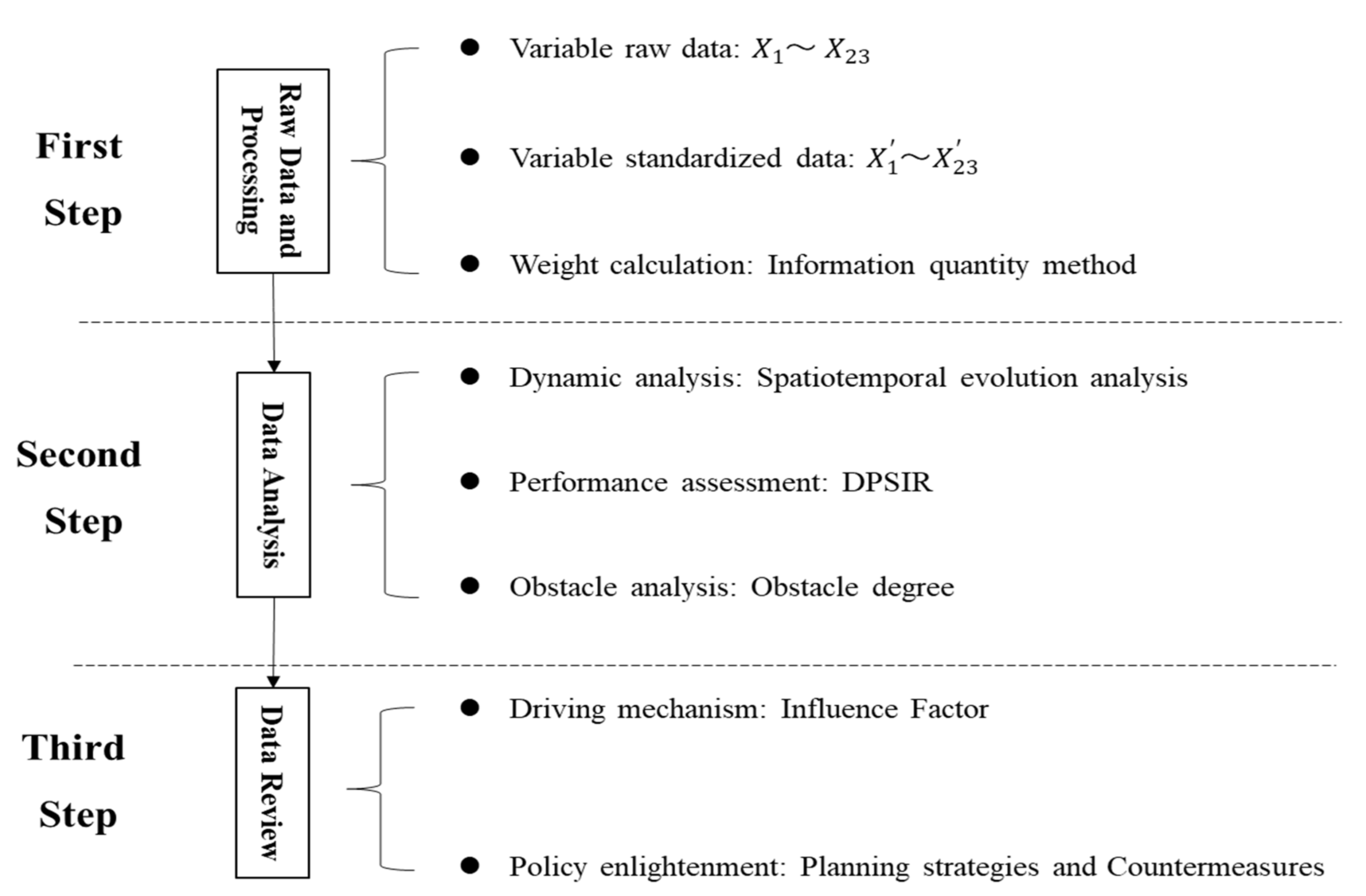
2.4. Research Steps and Data Sources

This study consists of three steps (Figure 5).

The first step is the raw data processing; that is, to create complete raw data tables using data published on statistical sites. Since the scale units of each index are different and the indexes cannot be directly compared with each other, Equations (3) and (4) were applied to standardize the positive and negative indexes, respectively. As the research on the performance of real estate inventory management using the DPSIR model is still an emerging field, we currently only know that there should be differences among indexes, but we are still unable to determine the degree of differences in importance between them. It is very simple and convenient to calculate the weight based on the information content method. Using the information content within the data to identify the index weights applies to both large and small samples of data. For an exploratory study of real estate inventory management performance evaluation in this paper, to calculate the weights by the information content method is a good solution to open the “black box”. The coefficient of variation of each index is first calculated, then it is normalized, and the new value obtained is used as the weight. The coefficient of variation is the core of the method, and generally the weight assigned is greater when the coefficient of variation is larger. In this paper, we calculate the weights by information content, and calculate the weighting results using the software SPSSAU.

The second step is data analysis, including Dynamic Analysis, Performance Assessment, and Obstacle Analysis. Dynamic Analysis includes both time series analysis and spatial analysis. The former studies the development trend based on data changes from 2010 to 2019, while the latter studies the spatial characteristics based on the coefficient of variation and spatial clustering. We should note that the coefficient of variation is an important index to measure spatial heterogeneity, and its trend can also better reflect the characteristics of convergence. According to the research by Guan [110], Zhang [111], Ruan [112], Liu [113], Miyamoto [114], and She [115], dispersion is classified into weak, medium, and strong levels based on the CV values. That is, a CV value of 0–0.15 shows weak dispersion, reflecting a low degree of spatial inequality of urbanization; a value of 0.16–0.35 shows medium dispersion, reflecting a high degree of spatial inequality of urbanization; a value of 0.36 or more shows strong dispersion, reflecting a very high degree of spatial inequality of urbanization. Performance Assessment includes real estate inventory management performance rating analysis and spatial clustering analysis, while Obstacle Analysis includes analysis of the critical obstacle factors to real estate destocking management and comparative analysis of the differences between different regions.

The third step is data review. This section discusses the real estate inventory management performance and influence factors in China, and proposes optimization strategies or policy insights for real estate inventory management. This is a summary of the analysis of the results in Section 3, drawing a conclusion that is broadly applicable, replicable, and worthy for popularization. We also present some policy suggestions here based on our analysis to lay the foundation for the government and enterprises to apply the findings of this paper for real estate inventory management.

The indexes in this paper mainly come from the China Real Estate Statistics Yearbook, China Statistical Yearbook, China City Statistical Yearbook, and China Urban Construction Statistical Yearbook. Some missing data were collected from provincial and city statistical yearbooks, statistical bulletins, and government work reports. There are two main reasons for setting the study period from 2010 to 2019. One is to ensure the consistency of the statistical caliber of the data. For example, in 2009, the National Bureau of Statistics adjusted the “vacant area of commercial buildings” to “area for sale”, and a prolonged research time would affect the accuracy of the conclusion due to poor comparison between the two indexes. The other is to maintain the relative consistency of the policy background. China’s housing market as a whole was under severe control from 2010 to 2019, when anti-overheating, financial retrenchment, destocking, and housing without speculation constituted the keynote policy; especially, a series of special policies on real estate destocking were implemented after 2015.

3. Results

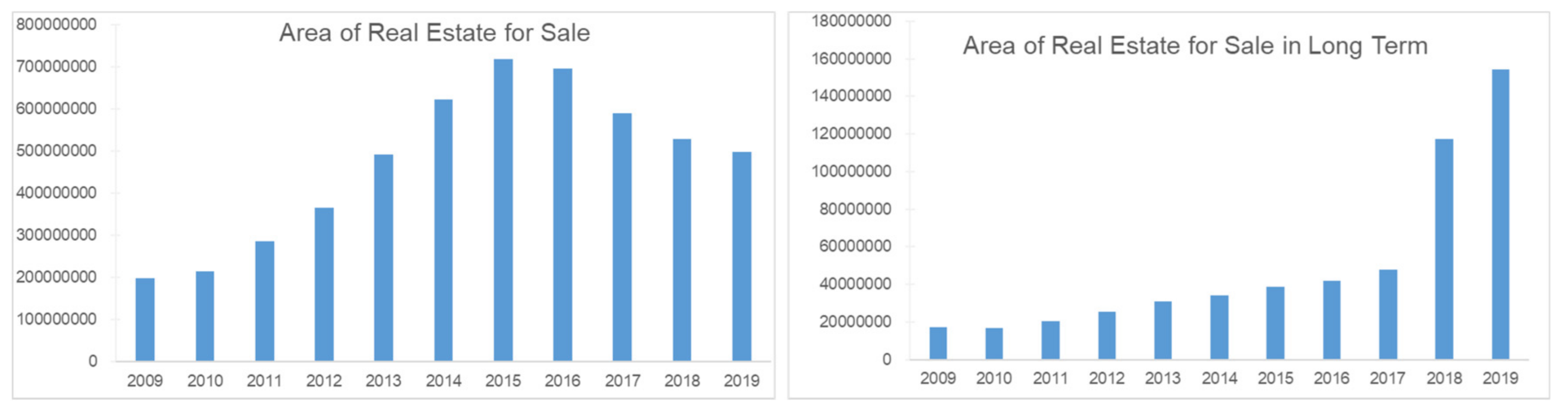
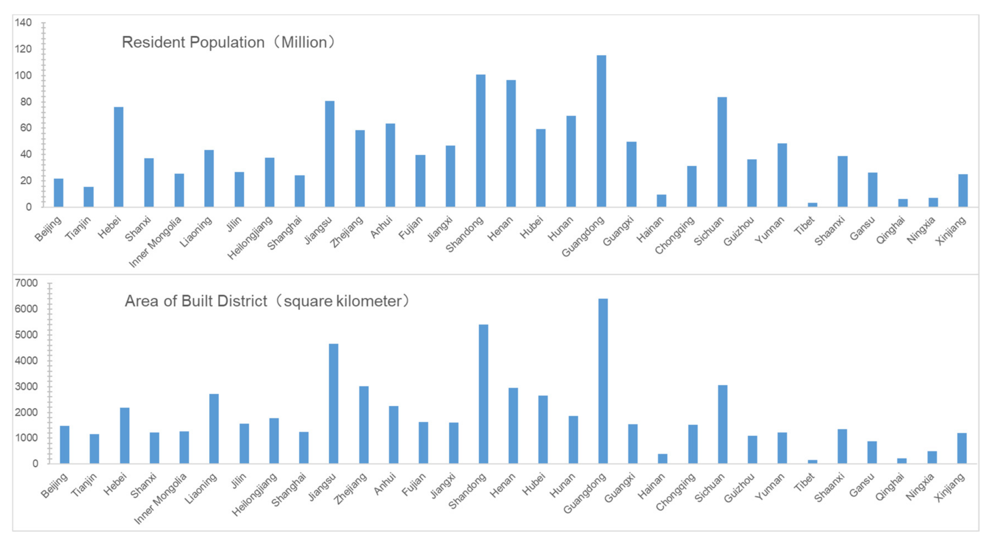
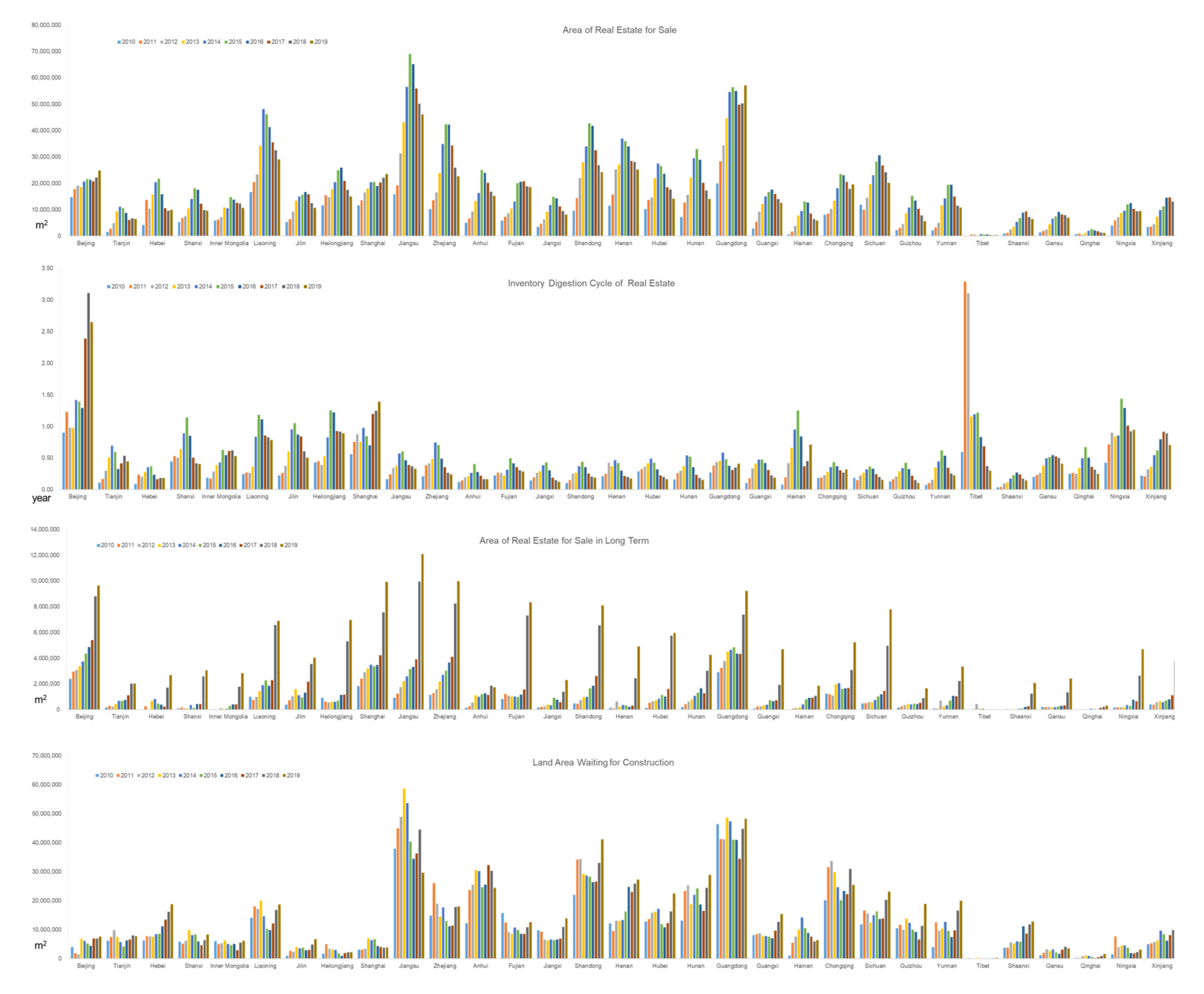
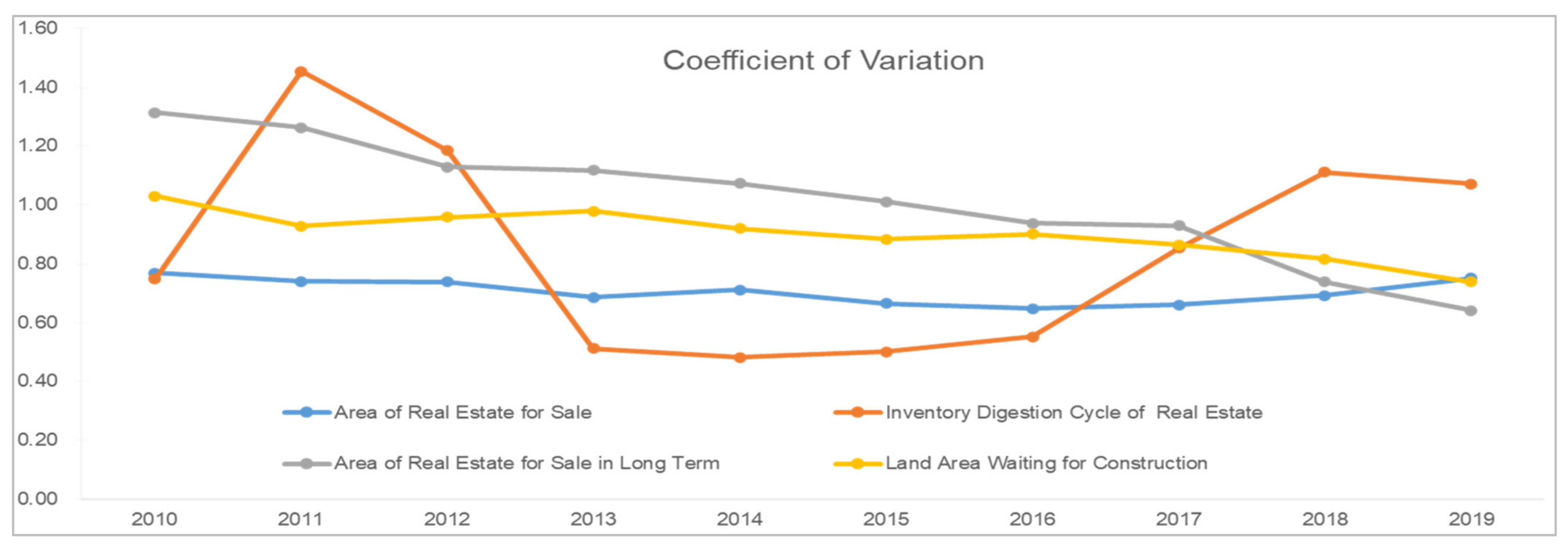
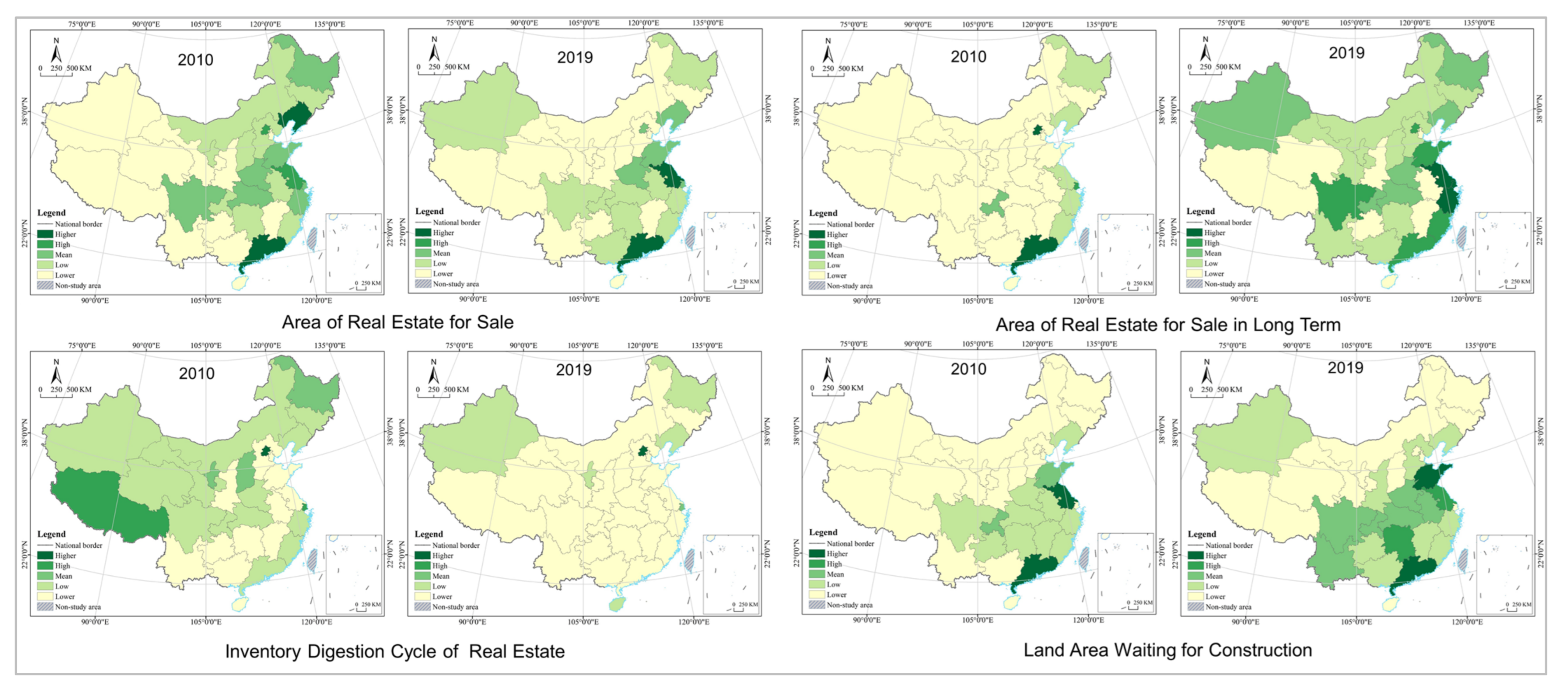
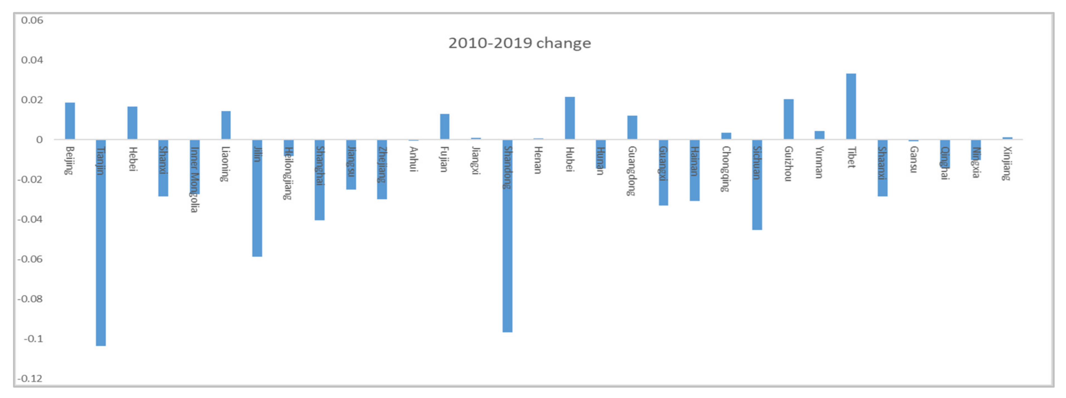
3.1. Spatial and Temporal Dynamic Analysis

From the perspective of Area of Real Estate for Sale, Jiangsu, Guangdong, and Liaoning have the largest inventory of real estate, followed by Zhejiang, Shandong, and Henan, which also have a large one. From 2010 to 2019, all provinces and cities in China, except Beijing and Shanghai, showed an “inverted U-shaped” trend under the intervention of real estate destocking policy (Figure 6). The coefficient of variation remained around 0.8 from 2010 to 2019, much larger than 0.36, indicating a very high degree of spatial inequality in the amount of real estate inventory [116] (Figure 7). According to the relative share of the real estate inventory scale ($\frac{X_j}{X_{max}}\times 100\%$), the 31 provinces and cities were divided into five levels with significant spatial differentiation and agglomeration [117] (Figure 8). In 2010, Guangdong and Liaoning were at the Higher level; Jiangsu and Beijing were at the High level; Sichuan, Heilongjiang, Shanghai, Henan, Hubei, Zhejiang, Shandong, and Chongqing were at the Mean level; Hunan, Inner Mongolia, Fujian, Jilin, Shanxi, Anhui, Hebei, and Ningxia were a the Low level; and Jiangxi, Xinjiang, Guangxi, Guizhou, Yunnan, Tianjin, Gansu, Shaanxi, Qinghai, Hainan, and Tibet were at the Lower level. In 2019, the regions of Lower level underwent a significant expansion; there were no High-level regions; the regions of Higher level were Guangdong and Jiangsu; the regions of Mean level were Shanghai, Shandong, Beijing, Henan, and Liaoning; and the regions of Low level were Zhejiang, Sichuan, Chongqing, Fujian, Anhui, Heilongjiang, Hubei, Hunan, Guangxi, and Xinjiang. The real estate in this paper includes houses for residential, office, commercial, industrial, and other purposes, which are used for market operation and sales, excluding public welfare buildings such as government, schools, hospitals, science and technology museums, and museums.

From the perspective of Inventory Digestion Cycle of Real Estate, Beijing and Tibet have the longest period of real estate destocking, much longer than 1.5 years, followed by Shanxi, Liaoning, Jilin, Heilongjiang, Shanghai, Hainan, Ningxia, and Xinjiang, which have a longer period, remaining at around 1 year for a long time. From 2010 to 2019, the destocking period of most provinces and cities showed an “inverted U-shaped” trend under the intervention of the real estate destocking policy. It is worth noting that Beijing and Shanghai showed a rapid upward trend in the fluctuation (Figure 6). The coefficient of variation fluctuated from 2010 to 2019, but always above 0.36, indicating a high degree of spatial inequality and a very unstable development of the real estate destocking period (Figure 7). In 2010, Beijing was at the Higher level; Tibet and Shanghai were at the High level; Heilongjiang, Shanxi, and Ningxia were at the Mean level; Jilin, Liaoning, Zhejiang, Fujian, Guangdong, Henan, Hubei, Qinghai, and Xinjiang were a the Low level; and most regions, such as Hainan, Guizhou, Jiangsu, and Tianjin, were at the Lower level. In 2019, Beijing was still the only region at the Higher level; no province or city was a the High level; Shanghai was the only region at the Mean level; regions at the Low level shrank greatly (only Heilongjiang, Liaoning, Hainan, Ningxia, and Xinjiang); and regions at the Lower level expanded significantly, showing a significant decrease in spatial complexity (Figure 8).

From the perspective of Area of Real Estate for Sale in Long Term, Jiangsu, Shanghai, Zhejiang, Fujian, Shandong, Guangdong, Sichuan, Beijing, Liaoning, and Heilongjiang have the largest inventory, followed by Ningxia, Xinjiang, Chongqing, and Hubei, which have a larger one. Different from the Area of Real Estate for Sale, the Area of Real Estate for Sale in Long Term in provinces and cities across China except Tibet generally has enjoyed a rapid growth, especially in the last two years (Figure 6). The coefficient of variation was in a continuous decline from 2010 to 2019, but always over 0.36, indicating that the spatial inequality of long-term real estate inventory was very high with spatial convergence (Figure 7). In 2010, Beijing and Guangdong were at the Higher level; Shanghai was the only region at the High level; Chongqing was the only region at the Mean level; Heilongjiang, Liaoning, Jiangsu, Zhejiang, and Fujian were at the Low level; and most regions, such as Shandong, Hebei, Hainan, and Shanghai, were at the Lower level. In 2019, regions at the Higher level were Jiangsu, Shanghai, and Zhejiang; Beijing, Tianjin, Shandong, Sichuan, Fujian, and Guangdong were at the High level; regions at the Mean level expanded to Heilongjiang, Liaoning, Henan, Hubei, and Xinjiang; regions at the Low level expanded significantly with the coverage of Yunnan, Guangxi, Hunan, Gansu, Ningxia, Inner Mongolia, Shanxi, and Hebei; and regions at the Lower level shrank significantly to only Hainan, Jiangxi, Anhui, Beijing, Tianjin, Shaanxi, Qinghai, and Tibet (Figure 8).

From the perspective of Land Area Waiting for Construction, real estate enterprises in Jiangsu, Guangdong, Shandong, Anhui, and Chongqing have the largest area, followed by those in Henan, Hunan, Sichuan, Liaoning, Hubei, and Yunnan, which also have a large one. From 2010 to 2019, the undeveloped land area of real estate enterprises in provinces and cities of China showed a variety of changing forms, including a J-shaped change in Hebei, Jilin, Shaanxi, and Xinjiang, U-shaped change in Liaoning, Jiangxi, and Fujian, inverted U-shaped change in Hainan, Shanghai, and Jiangsu, and wave-shaped change in Tianjin, Shanghai, and Inner Mongolia (Figure 6). The coefficient of variation showed a slow decline from 2010 to 2019, but still remaining above 0.8, much larger than 0.36, indicating a very high spatial inequality of undeveloped land of real estate enterprises with spatial convergence (Figure 7). In 2010, Guangdong and Jiangsu were at the Higher level; no regions were at the High level; Shandong and Chongqing were at the Mean level; Liaoning, Zhejiang, Fujian, and Anhui were at the Low level; and most regions, such as Hainan, Guangxi, Yunnan, and Xinjiang, were at the Lower level. In 2019, regions of Higher level were Shandong and Guangdong; only Jiangsu and Hunan were at the High level; regions at the Mean level expanded significantly with the coverage of Sichuan, Yunnan, and Hunan; and regions at the Lower level shrank slightly, but they were still highly concentrated (Figure 8).

In general, the spatio-temporal evolution of China’s real estate inventory is characterized by the following features: in terms of the evolution trend, Area of Real Estate for Sale and Inventory Digestion Cycle of Real Estate shows an “inverted U-shaped” change; Area of Real Estate for Sale in Long Term is dominated by “J-shaped” growth; while Land Area Waiting for Construction has diversified trends, such as “J-shaped”, “U-shaped” and “inverted U-shaped”. In terms of spatial distribution, the spatial heterogeneity and agglomeration of real estate inventories in China are prominent, with provinces having large total inventories clustered mainly in the coastal and riverine (Yangtze) regions, especially Jiangsu, Guangdong, Shanghai, Zhejiang, and Fujian. It is worth noting that China has a long and lengthening real estate destocking period, with long-term real estate inventory growing rapidly over the past two years.

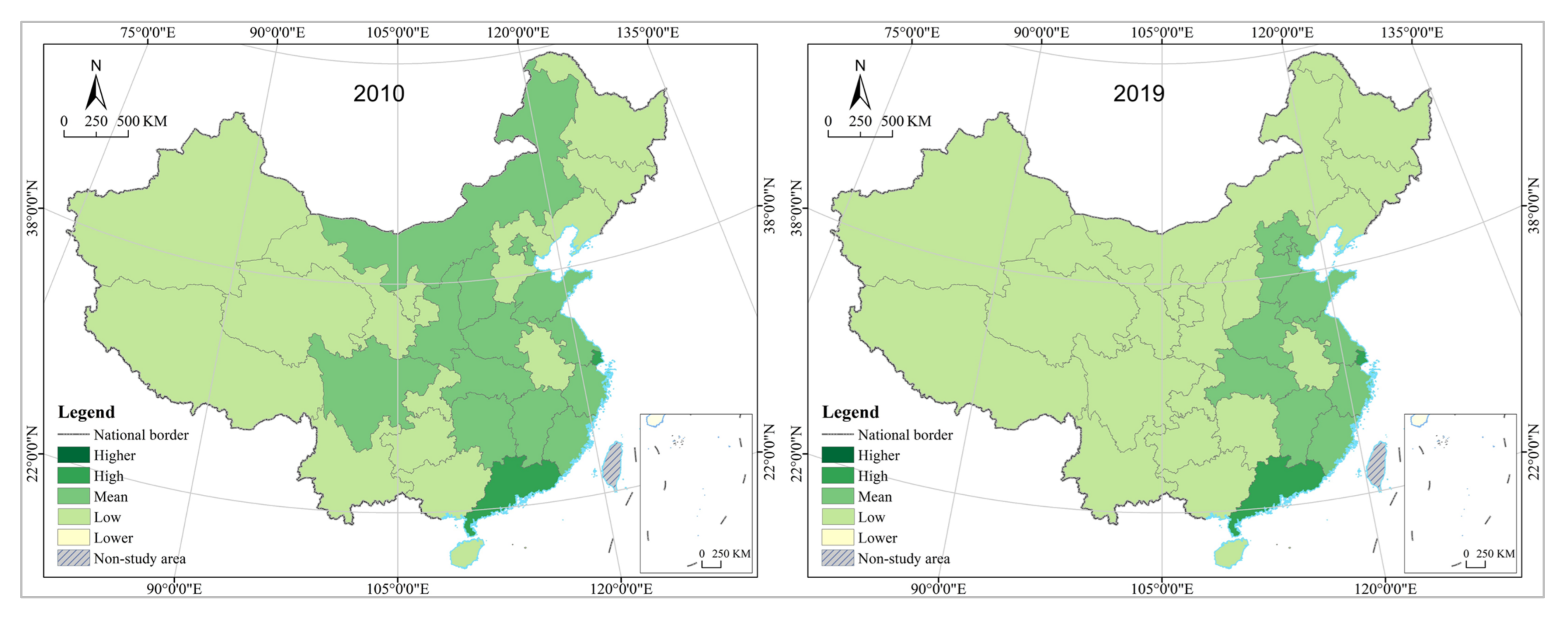
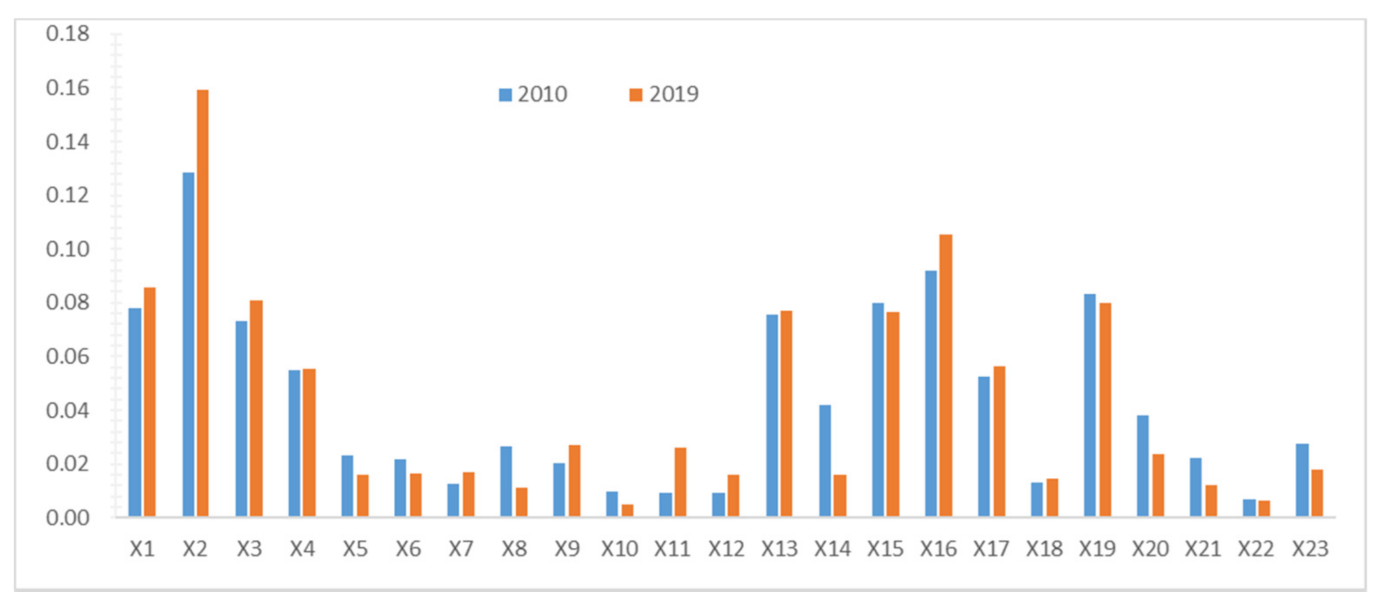
3.2. Performance and Obstacle Analysis

We calculated the real estate inventory management performance indexes of all provinces based on Equation (5) and averaged them to represent the general level of real estate inventory management performance in China (

Table 2. Performance evaluation of the real estate inventory management index in China.

		2010			2019
Code	Name	Index	Ranking	Light	Index	Ranking	Light
1	Beijing	0.5456	5	Yellow	0.5641	26	Yellow
2	Tianjin	0.5276	6	Yellow	0.4238	29	Yellow
3	Hebei	0.3957	17	Orange	0.4122	25	Yellow
4	Shanxi	0.4057	14	Yellow	0.3772	27	Orange
5	Inner Mongolia	0.4257	11	Yellow	0.3982	13	Orange
6	Liaoning	0.3822	21	Orange	0.3966	23	Orange
7	Jilin	0.3954	18	Orange	0.3367	20	Orange
8	Heilongjiang	0.3806	22	Orange	0.3724	22	Orange
9	Shanghai	0.6519	1	Blue	0.6115	17	Blue
10	Jiangsu	0.5750	3	Yellow	0.5500	18	Yellow
11	Zhejiang	0.5569	4	Yellow	0.5270	28	Yellow
12	Anhui	0.3671	26	Orange	0.3666	30	Orange
13	Fujian	0.4391	8	Yellow	0.4521	1	Yellow
14	Jiangxi	0.4027	15	Yellow	0.4034	14	Yellow
15	Shandong	0.4992	7	Yellow	0.4025	7	Yellow
16	Henan	0.4025	16	Yellow	0.4031	11	Yellow
17	Hubei	0.4224	12	Yellow	0.4438	12	Yellow
18	Hunan	0.4130	13	Yellow	0.3984	10	Orange
19	Guangdong	0.6350	2	Blue	0.6470	6	Blue
20	Guangxi	0.3784	23	Orange	0.3454	24	Orange
21	Hainan	0.3852	19	Orange	0.3544	5	Orange
22	Chongqing	0.3835	20	Orange	0.3871	4	Orange
23	Sichuan	0.4340	9	Yellow	0.3885	2	Orange
24	Guizhou	0.3520	30	Orange	0.3724	21	Orange
25	Yunnan	0.3717	25	Orange	0.3759	31	Orange
26	Tibet	0.3351	31	Orange	0.3683	16	Orange
27	Shaanxi	0.4277	10	Yellow	0.3991	15	Orange
28	Gansu	0.3572	27	Orange	0.3563	19	Orange
29	Qinghai	0.3759	24	Orange	0.3618	9	Orange
30	Ningxia	0.3566	28	Orange	0.3462	8	Orange
31	Xinjiang	0.3563	29	Orange	0.3576	3	Orange

). The average real estate inventory management performance index in China in 2010 was 0.43, with the maximum being 0.65 (Shanghai) and the minimum being 0.34 (Tibet). According to the classification criteria, there are no geographical areas at the Lower and Higher real estate inventory management performance levels in China. In 2010, Guangdong and Shanghai were at the High level; regions at the Mean and Low levels were concentrated in a contiguous distribution; regions at the Mean level were mainly distributed in the eastern coast and central China, including Beijing, Tianjin, Shandong, Jiangsu, Zhejiang, Fujian, Hunan, Hubei, Jiangxi, Henan, Shaanxi, Shanxi, Inner Mongolia, and Sichuan; and regions at the Low level were mainly distributed northeast, northwest, and southwest China, including Heilongjiang, Liaoning, Jilin, Hebei, Xinjiang, Gansu, Qinghai, Yunnan, Guangxi, Guizhou, Hainan, and Anhui (Figure 9). The average real estate inventory management performance index decreased to 0.42 in 2019, with the maximum being 0.65 (Guangdong) and the minimum being 0.34 (Jilin). According to the classification criteria, there were still no regions at the Lower and Higher levels; only Guangdong and Shanghai were regions at the High level; regions at the Mean level shrank significantly, with a concentrated, contiguous distribution in coastal areas and some parts of central China; and regions at the Low level underwent further expansion, mainly distributed in northwest, northeast, and southwest China. From the perspective of changes in real estate inventory management level from 2010 to 2019, Tibet, Beijing, Hebei, Liaoning, Hubei, Fujian, Guangdong, and Guizhou had a significant increase; Tianjin, Shandong, Jilin, Sichuan, Shanghai, Inner Mongolia, Shanxi, Jiangsu, Zhejiang, Guangxi, Hainan, and Shaanxi showed a significantly decrease; and Anhui, Jiangxi, Chongqing, Yunnan, Gansu, and Xinjiang remained stable (Figure 10).

We calculated the obstacle degree of each index to real estate inventory management based on Equations (1) and (2), with the results listed in

Table A1. Obstacle factor analysis of China’s real estate inventory management in 2010.

	${\mathit{X}}_1$	${\mathit{X}}_2$	${\mathit{X}}_3$	${\mathit{X}}_4$	${\mathit{X}}_5$	${\mathit{X}}_6$	${\mathit{X}}_7$	${\mathit{X}}_8$	${\mathit{X}}_9$	${\mathit{X}}_{10}$	${\mathit{X}}_{11}$	${\mathit{X}}_{12}$	${\mathit{X}}_{13}$	${\mathit{X}}_{14}$	${\mathit{X}}_{15}$	${\mathit{X}}_{16}$	${\mathit{X}}_{17}$	${\mathit{X}}_{18}$	${\mathit{X}}_{19}$	${\mathit{X}}_{20}$	${\mathit{X}}_{21}$	${\mathit{X}}_{22}$	${\mathit{X}}_{23}$
Beijing	0.09	0.22	0.00	0.10	0.00	0.01	0.01	0.00	0.01	0.04	0.06	0.01	0.10	0.02	0.10	0.00	0.07	0.01	0.08	0.00	0.01	0.05	0.01
Tianjin	0.10	0.18	0.07	0.08	0.00	0.01	0.01	0.01	0.01	0.00	0.01	0.01	0.10	0.03	0.10	0.09	0.07	0.01	0.09	0.00	0.01	0.01	0.01
Hebei	0.08	0.18	0.10	0.03	0.02	0.02	0.01	0.01	0.02	0.00	0.01	0.02	0.07	0.01	0.08	0.12	0.05	0.01	0.08	0.03	0.01	0.00	0.02
Shanxi	0.09	0.17	0.10	0.06	0.01	0.01	0.01	0.01	0.01	0.00	0.01	0.01	0.09	0.02	0.09	0.12	0.06	0.00	0.09	0.02	0.00	0.00	0.01
Inner Mongolia	0.10	0.18	0.08	0.07	0.01	0.01	0.00	0.01	0.01	0.00	0.01	0.01	0.09	0.03	0.10	0.10	0.06	0.01	0.10	0.02	0.00	0.00	0.01
Liaoning	0.09	0.17	0.09	0.06	0.01	0.01	0.01	0.01	0.02	0.01	0.03	0.02	0.08	0.02	0.08	0.11	0.06	0.00	0.08	0.02	0.01	0.00	0.01
Jilin	0.09	0.16	0.09	0.06	0.00	0.01	0.01	0.01	0.01	0.00	0.02	0.01	0.09	0.04	0.09	0.12	0.06	0.01	0.09	0.02	0.00	0.00	0.01
Heilongjiang	0.10	0.17	0.10	0.06	0.00	0.01	0.01	0.00	0.01	0.01	0.03	0.00	0.09	0.03	0.09	0.13	0.06	0.01	0.06	0.02	0.00	0.00	0.01
Shanghai	0.08	0.18	0.01	0.11	0.01	0.01	0.02	0.00	0.01	0.02	0.07	0.01	0.11	0.03	0.11	0.00	0.07	0.01	0.07	0.00	0.02	0.04	0.02
Jiangsu	0.05	0.12	0.05	0.04	0.04	0.05	0.06	0.03	0.08	0.00	0.07	0.04	0.01	0.02	0.02	0.10	0.03	0.06	0.03	0.02	0.04	0.01	0.04
Zhejiang	0.06	0.15	0.06	0.06	0.03	0.03	0.03	0.03	0.05	0.00	0.06	0.02	0.06	0.02	0.05	0.05	0.05	0.03	0.04	0.02	0.03	0.01	0.04
Anhui	0.08	0.14	0.09	0.04	0.02	0.02	0.03	0.04	0.04	0.00	0.01	0.02	0.07	0.01	0.06	0.11	0.05	0.04	0.08	0.03	0.02	0.00	0.02
Fujian	0.10	0.16	0.05	0.06	0.01	0.02	0.02	0.01	0.03	0.00	0.04	0.01	0.07	0.01	0.07	0.10	0.07	0.01	0.09	0.02	0.02	0.01	0.02
Jiangxi	0.09	0.16	0.10	0.05	0.01	0.01	0.01	0.01	0.03	0.00	0.01	0.01	0.08	0.00	0.08	0.12	0.06	0.02	0.09	0.03	0.01	0.00	0.01
Shandong	0.06	0.15	0.08	0.01	0.05	0.04	0.05	0.04	0.06	0.00	0.04	0.04	0.04	0.02	0.03	0.10	0.03	0.03	0.06	0.02	0.02	0.00	0.04
Henan	0.08	0.14	0.09	0.01	0.03	0.03	0.03	0.01	0.06	0.00	0.02	0.03	0.05	0.01	0.05	0.13	0.04	0.01	0.08	0.03	0.02	0.00	0.04
Hubei	0.09	0.15	0.08	0.05	0.02	0.02	0.01	0.01	0.04	0.00	0.03	0.02	0.07	0.01	0.06	0.12	0.05	0.02	0.09	0.03	0.01	0.00	0.02
Hunan	0.09	0.16	0.09	0.04	0.02	0.02	0.02	0.02	0.04	0.00	0.02	0.03	0.07	0.01	0.07	0.11	0.05	0.01	0.08	0.03	0.01	0.00	0.02
Guangdong	0.00	0.00	0.10	0.00	0.06	0.08	0.08	0.03	0.11	0.01	0.07	0.08	0.00	0.03	0.00	0.14	0.00	0.04	0.00	0.02	0.07	0.02	0.08
Guangxi	0.09	0.16	0.09	0.05	0.01	0.01	0.01	0.01	0.03	0.00	0.02	0.01	0.08	0.02	0.08	0.11	0.05	0.02	0.08	0.03	0.01	0.00	0.01
Hainan	0.10	0.16	0.09	0.08	0.00	0.00	0.01	0.00	0.00	0.01	0.01	0.01	0.10	0.02	0.10	0.11	0.07	0.00	0.10	0.02	0.00	0.01	0.01
Chongqing	0.09	0.14	0.07	0.06	0.01	0.01	0.02	0.01	0.03	0.00	0.02	0.02	0.08	0.02	0.08	0.11	0.06	0.02	0.09	0.02	0.01	0.00	0.01
Sichuan	0.08	0.15	0.09	0.02	0.03	0.03	0.02	0.01	0.06	0.00	0.04	0.02	0.06	0.01	0.05	0.12	0.04	0.04	0.07	0.03	0.02	0.00	0.02
Guizhou	0.09	0.17	0.10	0.06	0.01	0.01	0.00	0.01	0.02	0.00	0.01	0.02	0.09	0.00	0.09	0.12	0.06	0.00	0.09	0.03	0.01	0.00	0.01
Yunnan	0.09	0.17	0.10	0.05	0.02	0.01	0.01	0.01	0.02	0.00	0.01	0.02	0.08	0.00	0.08	0.11	0.05	0.01	0.09	0.03	0.01	0.00	0.01
Tibet	0.11	0.17	0.09	0.08	0.00	0.00	0.00	0.00	0.00	0.00	0.00	0.00	0.10	0.00	0.10	0.11	0.07	0.00	0.10	0.05	0.00	0.00	0.00
Shaanxi	0.09	0.17	0.08	0.06	0.01	0.01	0.01	0.01	0.02	0.00	0.01	0.01	0.08	0.02	0.08	0.12	0.06	0.01	0.09	0.02	0.01	0.00	0.01
Gansu	0.10	0.17	0.10	0.06	0.01	0.01	0.00	0.00	0.01	0.00	0.01	0.00	0.09	0.02	0.09	0.12	0.06	0.01	0.09	0.03	0.00	0.00	0.01
Qinghai	0.11	0.17	0.09	0.08	0.00	0.00	0.00	0.00	0.00	0.00	0.00	0.00	0.10	0.02	0.10	0.12	0.08	0.00	0.10	0.03	0.00	0.00	0.00
Ningxia	0.10	0.17	0.09	0.08	0.00	0.00	0.00	0.00	0.00	0.01	0.02	0.00	0.10	0.01	0.10	0.11	0.08	0.00	0.10	0.02	0.00	0.00	0.00
Xinjiang	0.09	0.17	0.09	0.06	0.01	0.01	0.00	0.01	0.01	0.01	0.02	0.01	0.09	0.02	0.09	0.12	0.06	0.01	0.10	0.03	0.00	0.00	0.01

and

Table A2. Obstacle factor analysis of China’s real estate inventory management in 2019.

	$X_1$	$X_2$	$X_3$	$X_4$	$X_5$	$X_6$	$X_7$	$X_8$	$X_9$	$X_{10}$	$X_{11}$	$X_{12}$	$X_{13}$	$X_{14}$	$X_{15}$	$X_{16}$	$X_{17}$	$X_{18}$	$X_{19}$	$X_{20}$	$X_{21}$	$X_{22}$	$X_{23}$
Beijing	0.07	0.09	0.00	0.10	0.02	0.02	0.01	0.02	0.01	0.05	0.04	0.00	0.10	0.09	0.09	0.02	0.06	0.01	0.07	0.00	0.05	0.04	0.04
Tianjin	0.10	0.17	0.01	0.10	0.01	0.01	0.01	0.02	0.01	0.00	0.00	0.01	0.11	0.00	0.12	0.06	0.09	0.01	0.11	0.01	0.01	0.02	0.01
Hebei	0.08	0.14	0.08	0.03	0.04	0.03	0.02	0.06	0.02	0.00	0.00	0.00	0.06	0.05	0.07	0.10	0.04	0.01	0.08	0.04	0.03	0.00	0.03
Shanxi	0.09	0.16	0.08	0.06	0.01	0.01	0.01	0.02	0.01	0.02	0.00	0.00	0.09	0.03	0.09	0.11	0.06	0.00	0.10	0.04	0.01	0.00	0.02
Inner Mongolia	0.09	0.14	0.05	0.07	0.03	0.02	0.01	0.04	0.02	0.01	0.00	0.00	0.08	0.02	0.09	0.10	0.06	0.00	0.10	0.03	0.01	0.00	0.02
Liaoning	0.06	0.12	0.06	0.05	0.05	0.04	0.02	0.06	0.04	0.01	0.01	0.01	0.06	0.03	0.06	0.09	0.04	0.03	0.07	0.03	0.04	0.00	0.04
Jilin	0.09	0.15	0.07	0.06	0.01	0.01	0.01	0.02	0.01	0.01	0.01	0.00	0.09	0.03	0.09	0.11	0.06	0.01	0.10	0.03	0.01	0.00	0.01
Heilongjiang	0.09	0.14	0.08	0.05	0.02	0.01	0.01	0.02	0.01	0.02	0.01	0.00	0.08	0.04	0.08	0.11	0.05	0.01	0.10	0.03	0.01	0.00	0.02
Shanghai	0.07	0.00	0.00	0.12	0.02	0.03	0.01	0.01	0.02	0.04	0.04	0.00	0.11	0.12	0.12	0.00	0.06	0.02	0.06	0.00	0.04	0.05	0.05
Jiangsu	0.01	0.05	0.06	0.03	0.08	0.07	0.05	0.05	0.07	0.01	0.02	0.04	0.01	0.06	0.03	0.08	0.01	0.06	0.00	0.04	0.07	0.01	0.07
Zhejiang	0.06	0.09	0.06	0.06	0.04	0.05	0.02	0.05	0.03	0.01	0.02	0.02	0.06	0.07	0.06	0.04	0.05	0.03	0.01	0.04	0.05	0.02	0.07
Anhui	0.08	0.13	0.09	0.04	0.03	0.02	0.01	0.04	0.02	0.00	0.00	0.01	0.07	0.03	0.08	0.10	0.05	0.02	0.09	0.04	0.03	0.00	0.03
Fujian	0.09	0.14	0.07	0.06	0.02	0.02	0.01	0.03	0.01	0.01	0.01	0.01	0.08	0.04	0.08	0.07	0.07	0.01	0.09	0.03	0.02	0.01	0.03
Jiangxi	0.09	0.15	0.09	0.05	0.01	0.01	0.01	0.01	0.01	0.00	0.00	0.01	0.08	0.03	0.09	0.11	0.06	0.00	0.10	0.04	0.01	0.00	0.02
Shandong	0.05	0.13	0.07	0.01	0.06	0.05	0.03	0.06	0.06	0.00	0.01	0.02	0.02	0.06	0.02	0.09	0.03	0.02	0.05	0.05	0.05	0.00	0.06
Henan	0.07	0.14	0.09	0.01	0.03	0.03	0.02	0.05	0.03	0.01	0.00	0.01	0.05	0.05	0.06	0.10	0.03	0.01	0.08	0.05	0.03	0.00	0.04
Hubei	0.09	0.14	0.08	0.04	0.02	0.02	0.01	0.03	0.02	0.01	0.00	0.01	0.07	0.03	0.07	0.11	0.05	0.02	0.09	0.04	0.02	0.00	0.03
Hunan	0.08	0.15	0.09	0.03	0.03	0.02	0.01	0.02	0.02	0.01	0.00	0.01	0.07	0.03	0.07	0.10	0.05	0.01	0.09	0.05	0.02	0.00	0.03
Guangdong	0.00	0.06	0.09	0.00	0.06	0.07	0.04	0.05	0.06	0.02	0.06	0.06	0.00	0.08	0.00	0.09	0.00	0.03	0.01	0.04	0.07	0.02	0.09
Guangxi	0.09	0.14	0.09	0.05	0.02	0.02	0.01	0.02	0.01	0.00	0.00	0.01	0.08	0.03	0.09	0.09	0.06	0.02	0.09	0.05	0.01	0.00	0.03
Hainan	0.10	0.14	0.09	0.08	0.00	0.00	0.00	0.01	0.00	0.00	0.00	0.00	0.10	0.01	0.10	0.10	0.08	0.00	0.11	0.04	0.01	0.01	0.00
Chongqing	0.08	0.13	0.08	0.06	0.02	0.02	0.01	0.02	0.02	0.01	0.02	0.02	0.09	0.00	0.09	0.09	0.06	0.01	0.09	0.03	0.02	0.00	0.02
Sichuan	0.07	0.13	0.10	0.02	0.03	0.03	0.02	0.02	0.04	0.01	0.01	0.01	0.07	0.02	0.07	0.11	0.02	0.02	0.08	0.05	0.03	0.00	0.04
Guizhou	0.09	0.13	0.10	0.05	0.01	0.01	0.00	0.02	0.01	0.00	0.00	0.01	0.09	0.04	0.09	0.11	0.06	0.00	0.10	0.05	0.01	0.00	0.01
Yunnan	0.08	0.14	0.10	0.05	0.01	0.01	0.01	0.02	0.01	0.00	0.00	0.00	0.09	0.05	0.09	0.10	0.05	0.02	0.09	0.05	0.01	0.00	0.02
Tibet	0.10	0.14	0.09	0.08	0.00	0.00	0.00	0.00	0.00	0.02	0.00	0.00	0.09	0.04	0.10	0.10	0.07	0.00	0.11	0.06	0.00	0.00	0.00
Shaanxi	0.09	0.15	0.09	0.06	0.01	0.02	0.00	0.01	0.01	0.00	0.00	0.00	0.09	0.03	0.09	0.11	0.06	0.01	0.10	0.04	0.01	0.00	0.01
Gansu	0.09	0.15	0.09	0.06	0.01	0.00	0.00	0.01	0.00	0.01	0.00	0.00	0.09	0.05	0.09	0.11	0.06	0.00	0.10	0.05	0.00	0.00	0.01
Qinghai	0.10	0.15	0.08	0.08	0.00	0.00	0.00	0.00	0.00	0.01	0.00	0.00	0.10	0.02	0.10	0.11	0.08	0.00	0.11	0.04	0.00	0.00	0.00
Ningxia	0.10	0.15	0.08	0.08	0.01	0.00	0.00	0.01	0.00	0.01	0.00	0.00	0.09	0.04	0.10	0.10	0.08	0.00	0.10	0.04	0.00	0.00	0.00
Xinjiang	0.09	0.14	0.08	0.07	0.01	0.01	0.00	0.01	0.01	0.01	0.01	0.00	0.09	0.06	0.09	0.11	0.06	0.00	0.10	0.04	0.00	0.00	0.01

. Since there are many factors in the evaluation index system of China’s real estate inventory management level, this paper takes the indexes ranked in the top 5 obstacles as the critical factors. According to the different obstacle factors, the 31 provinces for 2010 were divided into three categories. The first category covers the widest geographical area, including Beijing, Tianjin, Hebei, Shanxi, Inner Mongolia, Liaoning, Jilin, Heilongjiang, Shanghai, Jiangsu, Zhejiang, Anhui, Fujian, Jiangxi, Shandong, Henan, Hubei, and Hunan. Their critical obstacle factors are New Construction Area of House, Building Construction Area of House, Completed Construction Area of House, Land Area Purchased by Real Estate Enterprises, and Area of Real Estate for Sale, reflecting the great impact of supply exceeding demand and historical inventory. The second category covers Hainan, Tibet, Shaanxi, Qinghai, Ningxia, Xinjiang, Guizhou, Yunnan, and Gansu, mainly underdeveloped areas in western China. Their critical obstacle factors are Financial Revenue (or Per Capital GDP), Profits of Real Estate Enterprises, Total Retail Sales of Social Consumer Goods, Disposable Income of Urban Residents, and Loans Balance of Financial Institutions, which reflect the great impact of lagging economic development. The third category covers Guangdong, Guangxi, Chongqing and Sichuan, and their critical obstacle factors are complex (Table A1).

The 31 provinces and cities for 2019 can be divided into five categories, with significant geographical differentiation and increasingly complex obstacle factors. The division is based on the commonness and dissimilarity of the obstacle factors. The first category covers Hebei, Shanxi, Jilin, Jiangxi, Anhui, Henan, Hubei, Hunan, Sichuan, Guizhou, and Yunnan. Their obstacle factors are Financial Revenue, Profits of Real Estate Enterprises, Per Capital GDP, Disposable Income of Urban Residents, and Loans Balance of Financial Institutions. The obstacle factors are reflected in the process of declining economic growth and structural transformation, in which the government’s reliance on land finance and companies’ pursuit of profits are coupled, resulting in a real estate supply that exceeds demand and does not match the current stage of industrialization, the size of the population, nor its income level. The second category covers Hainan, Tibet, Shaanxi, Qinghai, Ningxia, and Xinjiang, mainly the less developed areas in western China. Their critical obstacle factors include Financial Revenue, Profits of Real Estate Enterprises, Total Retail Sales of Social Consumer Goods, Disposable Income of Urban Residents, and Loans Balance of Financial Institutions. The difference with the first category is that consumption power has replaced the level of industrialization. The third category covers Liaoning, Heilongjiang, Shandong, Guangxi, Gansu, and Inner Mongolia. Their critical obstacle factors are Financial Revenue, Profits of Real Estate Enterprises, and Disposable Income of Urban Residents, supplemented by Per Capita GDP and Total Retail Sales of Social Consumer Goods. The fourth category covers Fujian, Chongqing, Beijing, Tianjin, and Shanghai. Their critical obstacle factors are Financial Revenue, Profits of Real Estate Enterprises and Gross Domestic Product, supplemented by Total Retail Sales of Social Consumer Goods and Loans Balance of Financial Institutes. The fifth category covers Jiangsu, Zhejiang, and Guangdong, and their critical barrier factors have a complex composition and are significantly different from those of other geographic regions (Table A2).

The evolution of China’s real estate inventory management performance generally shows the following characteristics. In terms of index changes, the real estate inventory management performance in China is at a low level with a downward trend. In terms of performance types, regions at the higher and lower levels never appear, regions at the high level remain unchanged, regions at the mean level are spatially clustered but cover a significantly contracted territory, and regions at the low level areas are rapidly expanding. In terms of the obstacle degree, the barrier factors of different regions vary widely and are becoming more complicated, especially the differentiation between coastal and western regions is becoming more significant. The historical inventory is the primary constraint for the eastern region, while the lower level of economic development is the biggest obstacle and challenge of destocking in the western region.

4. Discussion

4.1. Influence Factor

With the average obstacle degree of each province and city representing the overall obstacle degree of China’s real estate inventory management, and based on the comprehensive analysis of the calculated results, we can find that Profits of Real Estate Enterprises, Disposable Income of Urban Residents, Financial Revenue, Per Capita GDP, Resident Population, Gross Domestic Product, Total Retail Sales of Social Consumer Goods, Financial Expense, and Loans Balance of Financial Institutions are critical obstacle factors (Figure 11). Changes in the obstacle degree of each factor were significantly differentiated from 2010 to 2019. Specifically, Profits of Real Estate Enterprises, Area of Real Estate for Sale in Long Term, Disposable Income of Urban Residents, Financial Revenue, and Per Capita GDP had a further increase as obstacles, while GDP Growth Rate, GDP Growth Rate, Land Area Purchased by Real Estate Enterprises, Urbanization Rate of Population, Investment of Real Estate Enterprises, and Number of Real Estate Enterprises had a decline, with the rest of the factors remaining stable.

Some of the findings of the study support certain viewpoints of the existing papers. Zhao [118] conducted an empirical study based on GeoDetector and data from 35 key cities in China, finding that the factors influencing real estate inventories in Chinese cities are becoming increasingly diverse, with real estate market competition intensity, population size, government support, and social consumption vitality level having the strongest influence on inventories, and that different factors show the interaction between bifactor enhancement and non-linear enhancement, and the driving mechanism is becoming increasingly complex. Shen [119] analyzed the panel data of 35 key cities in China of 2004–2014, arguing that land supply has a significant positive impact on real estate destocking. Based on spatial autoregressive models and principal component analysis, Barreca [120] concluded that community services and retail activity have a large and positive impact on real estate inventory levels. Li [121] and Hoekstra [122] argued that population size, especially population structure, has a huge impact on the real estate markets in China and the Netherlands, and that the size of urban real estate inventories will further expand in the future as the population ages and the number of empty nesters increases. Wang [123], Hui [124], and Coskun [125] believed that real estate drags down the social consumption vitality in China and OECD countries (Organization for Economic Co-operation and Development), and significantly squeezes household consumption. Besides, some empirical results in this paper are inconsistent with the findings of existing studies, and they can be considered as an important addition to the theory of real estate inventory management as a new finding. For example, Cai [126] and Hidalgo [127] argued that real estate is closely associated with urbanization development, but this paper finds no significant connection between the population urbanization rate and real estate destocking. The obvious success of China’s household registration system reform in recent years may be an important reason for that. Wu [128] argued that the Chinese real estate market is not experiencing oversupply, and it is clear that this paper does not support this view. Such a discrepancy may stem from differences in the timing of the study and the selection of indexes.

Influenced by multiple factors such as government policies, corporate sales strategies, and residents’ house purchasing behaviors, the housing price is in a very complex relationship with inventories in China. Lazear [129] believed that there is a reverse correlation between real estate inventory and price, and a high housing price is the key factor affecting destocking, but the empirical results of this paper indicates that the housing price has no significant impact on inventory management. In other words, the housing price is not the critical obstacle to real estate destocking, and it is hard to achieve the destocking target by enforcing a lower housing price. There are two possible reasons to explain it: first, China’s housing prices are highly influenced by government and policy interventions, especially in recent years when the central and local governments have executed vigorous regulation and control over the real estate market; and second, there is a long-standing abnormal relationship between housing prices and real estate sales in China, and residents buy houses “when the prices are going up instead of going down”, which further leads to the complicated relationship between housing prices and inventory. To get a refined view on the relationship between the two, specialized empirical studies are needed in the future.

There are also some deficiencies in our research, which may affect the accuracy and applicability of some research conclusions in this paper. For example, in recent years, Chinese governments at all levels have intensively issued a series of real estate market development and governance policies, which have exerted a great impact on inventory management [130]. However, due to the difficulties in data acquisition and quantification, they are not included in the index system of this paper.

4.2. Policy Suggestion

Due to the huge scale and significant spatial variation in China’s real estate inventory, as well as the increasingly diverse and complex factors influencing inventory management, real estate destocking policies must be tailored to local conditions and a “one-size-fits-all” approach should not be allowed. The first step is to find out the real situation of the real estate market and get acquainted with the inventory quantity, inventory structure, inventory distribution, and companies with high inventory pressure in each province. The second step is that the central government should delegate more autonomy to local governments, so that they can formulate and implement differentiated real estate destocking policies according to local social and economic foundations and different development stages. The third step is to design differentiated policies based on the real conditions of supply and demand in the real estate market, focusing on coordinating the short-term and long-term goals of destocking, direct and indirect forces, and administrative and market means, so as to steadily improve the performance level of inventory management.

From the perspective of destocking goals, it is necessary to take into account and connect the relationship between short-term tactical objectives and long-term strategic objectives. The near-term goal is to achieve sustainable development of the real estate market, so it is required to control the investment scale and improve corporate profits, encourage mergers and acquisitions of real estate enterprises, improve industry concentration, and enhance the destocking capacity and financial risk tolerance of real estate enterprises. For example, tighten the financial support policies in the investment field of real estate enterprises, and moderately relax the conditions of residents’ house purchase loans. The long-term goal is to reduce the risks posed to the financial and economic system by high real estate inventories, so the government must take reasonable measures to accelerate economic development, increase GDP per capita, and promote high-quality industrialization and urbanization [131]. For example, reduce the proportion of real estate investment in urban investment, promote the decoupling between urban financial (or GDP) growth and real estate, and gradually resolve the dependence of urban economy on real estate.

We should note that the high inventory of real estate in China is not only a market economy phenomenon but also an issue involving politics and economics. The government plays a vital role in generating and clearing up the inventory of real estate. With its monopoly on urban land supply and over-reliance on “land finance”, the Chinese government has long adopted a land grant model similar to that of Hong Kong; i.e., restricting land supply to drive up land prices, resulting in structural imbalances in the real estate market. The coexistence of a high inventory and high housing price has become a popular phenomenon in China’s urban real estate market. From the results of obstacle degree analysis in the section above, government financial input and bank credit policy are significant and even critical obstacle factors in Shaanxi, Inner Mongolia, Qinghai, Ningxia, Tibet, Hainan, and Guizhou; the structure and scale of land supply also play a remarkable constraining role in Jiangsu, Zhejiang, Shandong, Guangdong, and Sichuan. Therefore, local and city governments must develop and implement destocking policies according to their local conditions. The first is to accelerate the reform of the government’s land supply system, for first- and second-tier cities and developed regions, to moderately expand the scale of land supply, while tightening the real estate supply in third- and fourth-tier cities and western regions. The second is to update the real estate purchase restriction policy; specifically, to standardize the purchase restriction policy in the first- and second-tier cities and keep it stable to prevent speculation caused by policy fluctuations. The third is to remove the house purchase quota policy in the third- and fourth-tier cities and less developed regions that are under great pressure to reduce inventory, and encourage purchasing houses and settling. The fourth is to reform financially, especially real estate credit-related policies, specifically for third- and fourth-tier cities and less developed regions with high real estate inventory pressure, to raise the share of housing provident fund loans, promote off-site loans, increase the loan amount, extend the loan term, relax the withdrawal conditions, reduce taxes, provide deed subsidies, reduce the down payment and interest rates, and make a rational use of financial leverage to meet and activate potential demand, to rebalance the market supply and demand; on the contrary, for the first- and second-tier cities and developed regions to strictly control speculative demand. The fifth is to change the government’s financial investment mode, increase investment in urban construction in third- and fourth-tier cities and less developed regions, and prioritize the strengthening of urban hardware facilities and the software environment, such as transportation, education, medical care, leisure, entertainment, culture, and security, to enhance the attractiveness to the population, and in turn to stimulate the demand for home ownership and achieve sustainable development of the real estate market.

From the perspective of destocking forces, the roles of direct and indirect driving forces should be integrated. It has been indicated in the previous section that population size, residents’ income level, and corporate profits are the critical obstacles affecting inventory management. Therefore, taking reasonable measures to improve the agglomeration, attractiveness, and carrying capacity of cities for the population should become a priority for the government in real estate destocking [132]. In addition, to improve the income and consumption ability of urban residents, to increase the supervision and regulation of the real estate market, to control the profitability of the industry and real estate prices, and to reduce the impulse of the society and the market to blindly invest in real estate are all relevant tasks that should not be ignored in real estate inventory management.

From the perspective of destocking measures, the government and market forces should be integrated, starting from both the supply side and demand side. Bao [133], Wang [134], Deng [135], Han [136], Jin [137], and Agunbiade [138] et al. analyzed the connection between supply-side land reserves, land finance, and real estate development, indirectly suggesting that land finance and land supply reform are the keys to destocking. This paper also finds that fiscal revenue and land supply are the critical obstacles to inventory management, showing that promoting the reform of land supply and financial system should be the core work of the government in the process of destocking [139], such as scientific preparation of annual plans for land supply, mastering the timing of land supply, controlling the scale of land supply, reducing “raw land” sales, and preventing excessive land allocation to reduce real estate inventory from the beginning [140,141]. Moreover, on the demand side, the influence of per capita GDP and GDP on real estate inventory management is increasing, which enlightens the government to take reasonable measures to improve the driving force of economic development, especially to promote industrialization, guide population agglomeration with industrial development, and create real estate consumption demand, thereby indirectly driving real estate destocking, and realizing the rebalancing of real estate market development.

5. Conclusions

Inventories of varying degrees can be found in real estate markets at present around the world, so it is of great theoretical and practical importance to reasonably evaluate inventory management performance and reveal its critical obstacle factors. With the help of the DPSIR framework, we constructed a real estate inventory management performance evaluation and obstacle diagnosis model based on multidimensional influence factors such as economic, social, and environmental elements, and conducted an empirical study on 31 provinces and cities in China, finding that the scale of real estate inventory in China is huge with significant spatial heterogeneity and agglomeration, the inventory management performance is unsatisfactory for a long time, the inter-provincial differences are large, and the inventory management barrier factors are becoming increasingly diversified and complex. Therefore, we propose the development of differentiated and precise response strategies based on the knowledge of the actual supply and demand in the real estate market and the integration of near-term and long-term goals, direct and indirect forces, and administrative and market instruments.

From a theoretical perspective, this study provides a new research framework and methodology for researchers in real estate economics, land management, human geography, spatial economics, and spatial planning, which facilitates revealing the patterns of real estate inventory management and its governance mechanisms [142].The current characteristics of an inventory are the core of real estate inventory management, but not all, and must be extended to the front end, focusing on the drive to create inventory and the pressure; and extended to the back end, considering the behavior of enterprises and governments in the face of inventory, as they are the key segments in the inventory management that should not be ignored. Past studies have been concerned only with inventory status evaluation, ignoring the front-end and back-end segments. The innovation of this paper is to incorporate the causes of inventory, current status, and response initiatives into a holistic framework, achieving a comprehensive study with full front-end–middle-end–back-end coverage. From a practical perspective, this paper analyzes the development trends and evolution laws of China’s real estate inventory, as well as the performance evaluation, obstacle diagnosis, and coping strategies of inventory management, which is helpful for policy makers and decision makers to find a scientific and reasonable real estate inventory governance model and provides the necessary decision basis for government management and policy regulation [143]. The research methods and findings of this paper are not only applicable to China but also can be used as a reference for decision making to solve the real estate inventory management problems in the United States, India, Japan, Mexico, Germany, the United Kingdom, Italy, and other countries.

References

1. Song, J.S.; van Houtum, G.J.; Van Mieghem, J.A. Capacity and Inventory Management: Review, Trends, and Projections. Manuf. Serv. Oper. Manag. 2020, 22, 36–46. [Google Scholar] [CrossRef]
2. Gutierrez, V.; Vidal, C.J. Inventory management models in supply chains: A literature review. Rev. Fac. Ing. Univ. Antioquia 2008, 43, 134–149. [Google Scholar]
3. Zhao, Y.; Wei, R.; Zhong, C.W. Research on Spatial Spillover Effects and Regional Differences of Urban Housing Price in China. Econ. Comput. Econ. Cybern. Stud. Res. 2021, 55, 211–228. [Google Scholar] [CrossRef]
4. Jang, H.; Song, Y.; Sohn, S.; Ahn, K. Real Estate Soars and Financial Crises: Recent Stories. Sustainability 2018, 10, 4559. [Google Scholar] [CrossRef] [Green Version]
5. Chen, K.; Song, Y.Y.; Pan, J.F.; Yang, G.L. Measuring destocking performance of the Chinese real estate industry: A DEA-Malmquist approach. Soc. Econ. Plan. Sci. 2020, 69, 100691. [Google Scholar] [CrossRef]
6. Ye, Y.; Ge, Y.Q. A bibliometric analysis of inventory management research based on knowledge mapping. Electron. Libr. 2019, 37, 127–154. [Google Scholar] [CrossRef]
7. Lopez, J.A.; Mendoza, A.; Masini, J. A Classic and Effective Approach to Inventory Management. Int. J. Ind. Eng. Theory Appl. Pract. 2013, 20, 372–386. [Google Scholar]
8. Yan, B.; Wu, J.W.; Liu, L.F.; Chen, Q.Q. Inventory Management Models in Cluster Supply Chains Based on System Dynamics. Rairo Oper. Res. 2017, 51, 763–778. [Google Scholar] [CrossRef]
9. Melikov, A.Z.; Shahmaliyev, M.O. Markov Models of Inventory Management Systems with a Positive Service Time. J. Comput. Syst. Sci. Int. 2018, 57, 766–783. [Google Scholar] [CrossRef]
10. Preil, D.; Krapp, M. Artificial intelligence-based inventory management: A Monte Carlo tree search approach. Ann. Oper. Res. 2021, 19, 1–25. [Google Scholar] [CrossRef]
11. Drakaki, M.; Tzionas, P. A Colored Petri Net-based modeling method for supply chain inventory management. Simul. Trans. Soc. Model. Simul. Int. 2021, 00375497211038755. [Google Scholar] [CrossRef]
12. Mamani, H.; Nassiri, S.; Wagner, M.R. Closed-Form Solutions for Robust Inventory Management. Manag. Sci. 2017, 63, 1625–1643. [Google Scholar] [CrossRef] [Green Version]
13. Borgonovo, E.; Peccati, L. Global sensitivity analysis in inventory management. Int. J. Prod. Econ. 2007, 108, 302–313. [Google Scholar] [CrossRef]
14. Hill, A.V.; Hang, W.Y.; Urch, G.F. Forecasting the forecastability quotient for inventory management. Int. J. Forecast. 2015, 31, 651–663. [Google Scholar] [CrossRef]
15. Subramanian, K.; Rawlings, J.B.; Maravelias, C.T. Economic model predictive control for inventory management in supply chains. Comput. Chem. Eng. 2014, 64, 71–80. [Google Scholar] [CrossRef]
16. Perez, H.D.; Hubbs, C.D.; Li, C.; Grossmann, I.E. Algorithmic Approaches to Inventory Management Optimization. Processes 2021, 9, 102. [Google Scholar] [CrossRef]
17. Borgonovo, E. Differential importance and comparative statics: An application to inventory management. Int. J. Prod. Econ. 2008, 111, 170–179. [Google Scholar] [CrossRef]
18. Almaktoom, A.T. Stochastic Reliability Measurement and Design Optimization of an Inventory Management System. Complexity 2017, 1460163. [Google Scholar] [CrossRef] [Green Version]
19. Jonsson, P.; Mattsson, S.A. An inherent differentiation and system level assessment approach to inventory management: A safety stock method comparison. Int. J. Logist. Manag. 2019, 30, 663–680. [Google Scholar] [CrossRef]
20. Lei, T.F.; Li, R.Y.M.; Fu, H.Y. Dynamics Analysis and Fractional-Order Approximate Entropy of Nonlinear Inventory Management Systems. Math. Probl. Eng. 2021, 2021, 5516703. [Google Scholar] [CrossRef]
21. Rahaman, M.; Mondal, S.P.; Alam, S.; Goswami, A. Synergetic study of inventory management problem in uncertain environment based on memory and learning effects. Sadhana Acad. Proc. Eng. Sci. 2021, 46, 39. [Google Scholar] [CrossRef]
22. Bendavid, I.; Herer, Y.T.; Yucesan, E. Inventory management under working capital constraints. J. Simul. 2017, 11, 62–74. [Google Scholar] [CrossRef]
23. Steinker, S.; Pesch, M.; Hoberg, K. Inventory management under financial distress: An empirical analysis. Int. J. Prod. Res. 2016, 54, 5182–5207. [Google Scholar] [CrossRef]
24. Katehakis, M.N.; Melamed, B.; Shi, J. Cash-Flow Based Dynamic Inventory Management. Prod. Oper. Manag. 2016, 25, 1558–1575. [Google Scholar] [CrossRef] [Green Version]
25. Sharma, S.; Abouee-Mehrizi, H.; Sartor, G. Inventory Management under Storage and Order Restrictions. Prod. Oper. Manag. 2020, 29, 101–117. [Google Scholar] [CrossRef]
26. Fu, K.; Gong, X.T.; Hsu, V.N.; Xue, J.Y. Dynamic Inventory Management with Inventory-based Financing. Prod. Oper. Manag. 2021, 30, 1313–1330. [Google Scholar] [CrossRef]
27. Buzacott, J.A.; Zhang, R.Q. Inventory management with asset-based financing. Manag. Sci. 2004, 50, 1274–1292. [Google Scholar] [CrossRef]
28. Herrmann, S.; Muhle-Karbe, J.; Shang, D.P.; Yang, C. Inventory Management for High-Frequency Trading with Imperfect Competition. Siam J. Financ. Math. 2020, 11, 1–26. [Google Scholar] [CrossRef]
29. Xu, C.; Duan, Y.R.; Huo, J.Z. Joint pricing and inventory management under servitisation. J. Oper. Res. Soc. 2019, 71, 893–909. [Google Scholar] [CrossRef]
30. Chen, Y.W.; Shi, C. Joint Pricing and Inventory Management with Strategic Customers. Oper. Res. 2019, 67, 1610–1627. [Google Scholar] [CrossRef]
31. Mokhtari, H. Joint ordering and reuse policy for reusable items inventory management. Sustain. Prod. Consum. 2018, 15, 163–172. [Google Scholar] [CrossRef]
32. Guo, S.; Choi, T.M.; Shen, B.; Jung, S.J. Inventory Management in Mass Customization Operations: A Review. IEEE Trans. Eng. Manag. 2019, 66, 412–428. [Google Scholar] [CrossRef]
33. Chen, X.; Hu, P.; Shum, S.; Zhang, Y.H. Dynamic Stochastic Inventory Management with Reference Price Effects. Oper. Res. 2016, 64, 1529–1536. [Google Scholar] [CrossRef] [Green Version]
34. Xiao, G.; Yang, N.; Zhang, R.Y. Dynamic Pricing and Inventory Management Under Fluctuating Procurement Costs. Manuf. Serv. Oper. Manag. 2015, 17, 321–334. [Google Scholar] [CrossRef] [Green Version]
35. Transchel, S. Inventory management underprice-based and stockout-based substitution. Eur. J. Oper. Res. 2017, 262, 996–1008. [Google Scholar] [CrossRef]
36. Park, S.; Huh, W.T.; Kim, B.C. Optimal inventory management with buy-one-give-one promotion. IISE Trans. 2021. [Google Scholar] [CrossRef]
37. Xie, C.; Wang, L.Q.; Yang, C.L. Robust inventory management with multiple supply sources. Eur. J. Oper. Res. 2021, 295, 463–474. [Google Scholar] [CrossRef]
38. Muharremoglu, A.; Yang, N. Inventory Management with an Exogenous Supply Process. Oper. Res. 2010, 58, 111–129. [Google Scholar] [CrossRef] [Green Version]
39. Mascle, C.; Gosse, J. Inventory management maximization based on sales forecast: Case study. Prod. Plan. Control. 2014, 25, 1039–1057. [Google Scholar] [CrossRef]
40. Nenes, G.; Panagiotidou, S.; Tagaras, G. Inventory management of multiple items with irregular demand: A case study. Eur. J. Oper. Res. 2010, 205, 313–324. [Google Scholar] [CrossRef]
41. Cao, Y.; Shen, Z.J.M. Quantile forecasting and data-driven inventory management under nonstationary demand. Oper. Res. Lett. 2019, 47, 465–472. [Google Scholar] [CrossRef]
42. Zhang, S.; Huang, K.; Yuan, Y.F. Spare Parts Inventory Management: A Literature Review. Sustainability 2021, 13, 2460. [Google Scholar] [CrossRef]
43. Muniz, L.R.; Conceicao, S.V.; Rodrigues, L.F.; Almeida, J.F.D.; Affonso, T.B. Spare parts inventory management: A new hybrid approach. Int. J. Logist. Manag. 2020, 32, 40–67. [Google Scholar] [CrossRef]
44. Turrini, L.; Meissner, J. Spare parts inventory management: New evidence from distribution fitting. Eur. J. Oper. Res. 2019, 273, 118–130. [Google Scholar] [CrossRef]
45. Kranenburg, A.A.; Van Houtum, G.J. Service differentiation in spare parts inventory management. J. Oper. Res. Soc. 2008, 59, 946–955. [Google Scholar] [CrossRef]
46. Dendauw, P.; Goeman, T.; Claeys, D.; De Turck, K.; Fiems, D.; Bruneel, H. Condition-based critical level policy for spare parts inventory management. Comput. Ind. Eng. 2021, 157, 107369. [Google Scholar] [CrossRef]
47. Zhang, F.; Guan, Z.L.; Zhang, L.; Cui, Y.Y.; Yi, P.X.; Ullah, S. Inventory management for a remanufacture-to-order production with multi-components (parts). J. Intell. Manuf. 2019, 30, 59–78. [Google Scholar] [CrossRef]
48. Aviles-Sacoto, S.V.; Aviles-Gonzalez, J.F.; Garcia-Reyes, H.; Bermeo-Samaniego, M.C.; Canizares-Jaramillo, A.K.; Izquierdo-Flores, S.N. A Glance of Industry 4.0 At Supply Chain and Inventory Management. Int. J. Ind. Eng. Theory Appl. Pract. 2019, 26, 486–506. [Google Scholar]
49. Fang, X.D.; Chen, H.C. Using vendor management inventory system for goods inventory management in IoT manufacturing. Enterp. Inf. Syst. 2021. [Google Scholar] [CrossRef]
50. Shan, J.; Zhu, K.J. Inventory Management in China: An Empirical Study. Prod. Oper. Manag. 2013, 22, 302–313. [Google Scholar] [CrossRef]
51. Swaminathan, A.M. Structural reforms and inventory management: Evidence from Indian industries. Int. J. Prod. Econ. 2001, 71, 67–78. [Google Scholar] [CrossRef]
52. Jaksic, M.; Fransoo, J.C. Optimal inventory management with supply backordering. Int. J. Prod. Econ. 2015, 159, 254–264. [Google Scholar] [CrossRef] [Green Version]
53. Agrawal, N.; Smith, S.A. Optimal inventory management for a retail chain with diverse store demands. Eur. J. Oper. Res. 2013, 225, 393–403. [Google Scholar] [CrossRef]
54. Ehrenthal, J.C.F.; Honhon, D.; Van Woensel, T. Demand seasonality in retail inventory management. Eur. J. Oper. Res. 2014, 238, 527–539. [Google Scholar] [CrossRef]
55. Turgut, O.; Taube, F.; Minner, S. Data-driven retail inventory management with backroom effect. Spectrum 2018, 40, 945–968. [Google Scholar] [CrossRef]
56. Saputro, T.E.; Figueira, G.; Almada-Lobo, B. Integrating supplier selection with inventory management under supply disruptions. Int. J. Prod. Res. 2020, 59, 3304–3322. [Google Scholar] [CrossRef]
57. Sarkar, S.; Kumar, S. A behavioral experiment on inventory management with supply chain disruption. Int. J. Prod. Econ. 2015, 169, 169–178. [Google Scholar] [CrossRef]
58. DeCroix, G.A. Inventory Management for an Assembly System Subject to Supply Disruptions. Manag. Sci. 2013, 59, 2079–2092. [Google Scholar] [CrossRef]
59. Hasan, M.R.; Daryanto, Y.; Roy, T.C.; Feng, Y. Inventory management with online payment and preorder discounts. Ind. Manag. Data Syst. 2020, 120, 2001–2023. [Google Scholar] [CrossRef]
60. Raviv, T.; Kolka, O. Optimal inventory management of a bike-sharing station. IIE Trans. 2013, 45, 1077–1093. [Google Scholar] [CrossRef]
61. Swaszek, R.M.A.; Cassandras, C.G. Receding Horizon Control for Station Inventory Management in a Bike-Sharing System. IEEE Trans. Autom. Sci. Eng. 2020, 17, 407–417. [Google Scholar] [CrossRef]
62. Chuang, C.H.; Zhao, Y.B. Demand stimulation in finished-goods inventory management: Empirical evidence from General Motors dealerships. Int. J. Prod. Econ. 2019, 208, 208–220. [Google Scholar] [CrossRef]
63. Mostafaei, H.; Castro, P.M.; Relvas, S.; Harjunkoski, I. A holistic MILP model for scheduling and inventory management of a multiproduct oil distribution system. Omega Int. J. Manag. Sci. 2021, 98, 102110. [Google Scholar] [CrossRef]
64. Siddiqui, A.; Verma, M.; Verter, V. An integrated framework for inventory management and transportation of refined petroleum products: Pipeline or marine? Appl. Math. Model. 2018, 55, 224–247. [Google Scholar] [CrossRef]
65. Dimas, D.; Murata, V.V.; Neiro, S.M.S.; Relvas, S.; Barbosa-Povoa, A.P. Multiproduct pipeline scheduling integrating for inbound and outbound inventory management. Comput. Chem. Eng. 2018, 115, 377–396. [Google Scholar] [CrossRef]
66. Toyasaki, F.; Arikan, E.; Silbermayr, L.; Sigala, I.F. Disaster Relief Inventory Management: Horizontal Cooperation between Humanitarian Organizations. Prod. Oper. Manag. 2017, 26, 1221–1237. [Google Scholar] [CrossRef] [Green Version]
67. Loree, N.; Aros-Vera, F. Points of distribution location and inventory management model for Post-Disaster Humanitarian Logistics. Transp. Res. Part E Logist. Transp. Rev. 2018, 116, 1–24. [Google Scholar] [CrossRef]
68. Natarajan, K.V.; Swaminathan, J.M. Inventory Management in Humanitarian Operations: Impact of Amount, Schedule, and Uncertainty in Funding. Manuf. Serv. Oper. Manag. 2014, 16, 595–603. [Google Scholar] [CrossRef]
69. Paam, P.; Berretta, R.; Heydar, M.; Garcia-Flores, R. The impact of inventory management on economic and environmental sustainability in the apple industry. Comput. Electron. Agric. 2019, 163, 104848. [Google Scholar] [CrossRef]
70. Golas, Z. The effect of inventory management on profitability: Evidence from the Polish food industry: Case study. Agric. Econ. Zemed. Ekon. 2020, 66, 234–242. [Google Scholar] [CrossRef]
71. Geman, H.; Tunaru, R. Commercial Real-Estate Inventory and Theory of Storage. J. Futures Mark. 2013, 33, 675–694. [Google Scholar] [CrossRef]
72. Pham, T.H.V.; Nguyen, M.H.V. Impact of Inventory Size, Staging, and Financing Policies on Sales Growth of Real Estate Companies in Vietnam . J. Glob. Econ. Bus. Financ. 2021, 3. [Google Scholar] [CrossRef]
73. Bian, X.; Waller, B.D.; Turnbull, G.K.; Wentland, S.A. How many listings are too many? Agent inventory externalities and the residential housing market. J. Hous. Econ. 2015, 28, 130–143. [Google Scholar] [CrossRef]
74. Caplin, A.; Leahy, J. Trading Frictions and House Price Dynamics. J. Money Credit Bank. 2011, 43, 283–303. [Google Scholar] [CrossRef] [Green Version]
75. Ott, S.H.; Hughen, W.K.; Read, D.C. Optimal Phasing and Inventory Decisions for Large-Scale Residential Development Projects. J. Real Estate Financ. Econ. 2012, 45, 888–918. [Google Scholar] [CrossRef]
76. Wen, X.Q.; Xu, C.; Hu, Q.Y. Dynamic capacity management with uncertain demand and dynamic price. Int. J. Prod. Econ. 2016, 175, 121–131. [Google Scholar] [CrossRef]
77. Kwoun, M.J.; Lee, S.H.; Kim, J.H. Dynamic cycles of unsold new housing stocks, investment in housing, and housing supply-demand. Math. Comput. Model. 2013, 57, 2094–2105. [Google Scholar] [CrossRef]
78. Morales, M.; Moraga, G.; Kirchheim, A.P.; Passuello, A. Regionalized inventory data in LCA of public housing: A comparison between two conventional typologies in southern Brazil. J. Clean. Prod. 2019, 238, 117869. [Google Scholar] [CrossRef]
79. Jiang, Y.X.; Zheng, L.Y.; Wang, J.Z. Research on external financial risk measurement of China real estate. Int. J. Financ. Econ. 2020, 26, 5472–5484. [Google Scholar] [CrossRef]
80. Muczynski, A. Financial flow models in municipal housing stock management in Poland. Land Use Policy 2020, 91, 104429. [Google Scholar] [CrossRef]
81. Yoo, H.; Yoon, H. The Effect of Green Characteristics in Reducing the Inventory of Unsold Housing in New Residential Developments-A Case of Gyeonggi Province, in South Korea. Land 2021, 10, 377. [Google Scholar] [CrossRef]
82. Nam, J.; Han, J.; Lee, C. Factors Contributing to Residential Vacancy and Some Approaches to Management in Gyeonggi Province, Korea. Sustainability 2016, 8, 367. [Google Scholar] [CrossRef] [Green Version]
83. Chen, C.; Wang, K.; Feng, M. Research on China’s Industrial Green Development based on the Pressure-State-Response Model. J. Sci. Ind. Res. 2020, 79, 541–546. [Google Scholar]
84. Tscherning, K.; Helming, K.; Krippner, B.; Sieber, S.; Paloma, S.G.Y. Does research applying the DPSIR framework support decision making? Land Use Policy 2012, 29, 102–110. [Google Scholar] [CrossRef]
85. Sekovski, I.; Newton, A.; Dennison, W.C. Megacities in the coastal zone: Using a driver-pressure-state-impact-response framework to address complex environmental problems. Estuar. Coast. Shelf Sci. 2012, 96, 48–59. [Google Scholar] [CrossRef]
86. Malekmohammadi, B.; Jahanishakib, F. Vulnerability assessment of wetland landscape ecosystem services using driver-pressure-state-impact-response (DPSIR) model. Ecol. Indic. 2017, 82, 293–303. [Google Scholar] [CrossRef]
87. Borji, M.; Nia, A.M.; Malekian, A.; Salajegheh, A.; Khalighi, S. Comprehensive evaluation of groundwater resources based on DPSIR conceptual framework. Arab. J. Geosci. 2018, 11, 158. [Google Scholar] [CrossRef]
88. Gupta, J.; Scholtens, J.; Perch, L.; Dankelman, I.; Seager, J.; Sander, F.; Stanley-Jones, M.; Kempf, I. Re-imagining the driver-pressure-state-impact-response framework from an equity and inclusive development perspective. Sustain. Sci. 2020, 15, 503–520. [Google Scholar] [CrossRef] [Green Version]
89. Carr, E.R.; Wingard, P.M.; Yorty, S.C.; Thompson, M.C.; Jensen, N.K.; Roberson, J. Applying DPSIR to sustainable development. Int. J. Sustain. Dev. World Ecol. 2007, 14, 543–555. [Google Scholar] [CrossRef]
90. Pan, W.Y.; Gulzar, M.A.; Hassan, W. Synthetic Evaluation of China’s Regional Low-Carbon Economy Challenges by Driver-Pressure-State-Impact-Response Model. Int. J. Environ. Res. Public Health 2020, 17, 5463. [Google Scholar] [CrossRef]
91. Padash, A.; Vahidi, H.; Fattahi, R.; Nematollahi, H. Analyzing and Evaluating Industrial Ecology Development Model in Iran Using FAHP-DPSIR. Int. J. Environ. Res. 2021, 15, 615–629. [Google Scholar] [CrossRef]
92. Liu, L.; Zhang, Q.; Wang, C.L.; Zhang, K.; Zhang, X. Comprehensive Eco-Environmental Impact Assessment of Urban Planning Based on Pressure-State-Response Model. Appl. Ecol. Environ. Res. 2019, 17, 14455–14463. [Google Scholar] [CrossRef]
93. Wang, D.; Shen, Y.; Zhao, Y.Y.; He, W.; Liu, X.; Qian, X.Y.; Lv, T. Integrated assessment and obstacle factor diagnosis of China’s scientific coal production capacity based on the PSR sustainability framework. Resour. Policy 2020, 68, 101794. [Google Scholar] [CrossRef]
94. Xie, X.; Fang, B.; Li, X.; He, S.S. Urban ecosystem health assessment and obstacle factor diagnosis using a comprehensive assessment model for Nanjing, China. Growth Chang. 2021, 52, 1938–1954. [Google Scholar] [CrossRef]
95. Cui, X.F.; Yang, S.; Zhang, G.H.; Liang, B.; Li, F. An Exploration of a Synthetic Construction Land Use Quality Evaluation Based on Economic-Social-Ecological Coupling Perspective: A Case Study in Major Chinese Cities. Int. J. Environ. Res. Public Health 2020, 17, 3663. [Google Scholar] [CrossRef]
96. Wang, H.N.; Zhang, M.Y.; Cui, L.J.; Guo, Z.L.; Wang, D.A. Evaluation of Ecological Environment Quality of Hengshui Lake Wetlands based on DPSIR Model. Wetl. Sci. 2019, 17, 193–198. [Google Scholar] [CrossRef]
97. Yang, J.S. An Empirical Study on The Relationship Between Taizhou’s Economic Development and Water Environment Pollution Based on the PSR Framework. J. Environ. Prot. Ecol. 2020, 21, 1146–1155. [Google Scholar]
98. Upreti, B.R.; Breu, T.; Ghale, Y. New Challenges in Land Use in Nepal: Reflections on the Booming Real-estate Sector in Chitwan and Kathmandu Valley. Scott. Geogr. J. 2017, 133, 69–82. [Google Scholar] [CrossRef]
99. Fernandez, M.D.; Marron, M.L.; Rodriguez, P.M. Does the population determine the dynamics of the real estate activity? An analysis of cointegration for the Spanish case. Investig. Econ. 2016, 75, 103–124. [Google Scholar] [CrossRef] [Green Version]
100. Klett, I.R.G. Urban land market and financial reserve of land for housing production in the Metropolitan Area of Santiago. Rev. Geogr. Norte Gd. 2020, 76, 71–94. [Google Scholar]
101. Chinloy, P.; Wu, Z.H. The Inventory-Sales Ratio and Homebuilder Return Predictability. J. Real Estate Financ. Econ. 2013, 46, 397–423. [Google Scholar] [CrossRef]
102. Pan, J.N.; Huang, J.T.; Chiang, T.F. Empirical study of the local government deficit, land finance and real estate markets in China. China Econ. Rev. 2015, 32, 57–67. [Google Scholar] [CrossRef]
103. Sinai, T. Feedback Between Real Estate and Urban Economics. J. Reg. Sci. 2010, 50, 423–448. [Google Scholar] [CrossRef]
104. Zhang, P.; Li, W.; Zhao, K.; Zhao, S. Spatial Pattern and Driving Mechanism of Urban–Rural Income Gap in Gansu Province of China. Land 2021, 10, 1002. [Google Scholar] [CrossRef]
105. Zhang, C.C.; Jia, S.; Yang, R.D. Housing affordability and housing vacancy in China: The role of income inequality. J. Hous. Econ. 2016, 33, 4–14. [Google Scholar] [CrossRef]
106. Hu, F.Z.Y.; Qian, J.W. Land-based finance, fiscal autonomy and land supply for affordable housing in urban China: A prefecture-level analysis. Land Use Policy 2017, 69, 454–460. [Google Scholar] [CrossRef]
107. Su, X.; Qian, Z. State Intervention in Land Supply and Its Impact on Real Estate Investment in China: Evidence from Prefecture-Level Cities. Sustainability 2020, 12, 1019. [Google Scholar] [CrossRef] [Green Version]
108. Wang, L.; Li, S.W.; Wang, J.N.; Meng, Y. Real estate bubbles in a bank-real estate loan network model integrating economic cycle and macro-prudential stress testing. Phys. A Stat. Mech. Appl. 2020, 542, 122576. [Google Scholar] [CrossRef]
109. Liu, T.Y.; Su, C.W.; Chang, H.L.; Chu, C.C. Is urbanization improving real estate investment? A cross-regional study of China. Rev. Dev. Econ. 2018, 22, 862–878. [Google Scholar] [CrossRef]
110. Guan, X.Y.; Wang, S.L.; Gao, Z.Y.; Lv, Y.; Fu, X.J. Spatio-temporal variability of soil salinity and its relationship with the depth to groundwater in salinization irrigation district. Acta Ecol. Sin. 2012, 32, 198–206. [Google Scholar]
111. Zhang, R.F. Theory and Application of Spatial Variability; Science Press: Beijing, China, 2005; pp. 13–14. [Google Scholar]
112. Ruan, B.Q.; Xu, F.R.; Jiang, R.F. Analysis on spatial and temporal variability of groundwater level based on spherical sampling model. J. Hydraul. Eng. 2008, 39, 573–579. [Google Scholar]
113. Liu, X.N.; Huang, F.; Wang, P. Spatial Analysis Principle and Method of GIS; Science Press: Beijing, China, 2008; pp. 199–206. [Google Scholar]
114. Miyamoto, S.; Chacon, A.; Hossain, M.; Martinez, L. Soil salinity of urban turf areas irrigated with saline water I. Spatial variability. Landsc. Urban Plan. 2005, 71, 233–241. [Google Scholar]
115. She, D.L.; Shao, M.A.; Yu, S.G. Spatial Variability of Soil Water Content on a Cropland-grassland Mixed Slope Land in the Loess Plateau, China. Trans. Chin. Soc. Agric. Mach. 2010, 41, 57–63. [Google Scholar]
116. Zhao, S.; Yan, Y.; Han, J. Industrial Land Change in Chinese Silk Road Cities and Its Influence on Environments. Land 2021, 10, 806. [Google Scholar] [CrossRef]
117. Zhao, S.; Zhang, P.; Li, W. A Study on Evaluation of Influencing Factors for Sustainable Development of Smart Construction Enterprises: Case Study from China. Buildings 2021, 11, 221. [Google Scholar] [CrossRef]
118. Zhao, S.D.; Li, W.W.; Zhao, K.X.; Zhang, P. Change Characteristics and Multilevel Influencing Factors of Real Estate Inventory-Case Studies from 35 Key Cities in China. Land 2021, 10, 928. [Google Scholar] [CrossRef]
119. Shen, X.Y.; Huang, X.J.; Li, H.; Li, Y.; Zhao, X.F. Exploring the relationship between urban land supply and housing stock: Evidence from 35 cities in China. Habitat Int. 2018, 77, 80–89. [Google Scholar] [CrossRef]
120. Barreca, A.; Curto, R.; Rolando, D. Is the Real Estate Market of New Housing Stock Influenced by Urban Vibrancy? Complexity 2020, 2020, 1908698. [Google Scholar] [CrossRef]
121. Li, M.; Shen, K.R. Population Aging and Housing Consumption: A Nonlinear Relationship in China. China World Econ. 2013, 21, 60–77. [Google Scholar] [CrossRef]
122. Hoekstra, M.S.; Hochstenbach, C.; Bontje, M.A.; Musterd, S. Shrinkage and housing inequality: Policy responses to population decline and class change. J. Urban Aff. 2020, 42, 333–350. [Google Scholar] [CrossRef]
123. Wang, Y.; Zhou, Y.; Yu, X.X.; Liu, X. Is domestic consumption dragged down by real estate sector? -Evidence from Chinese household wealth. Int. Rev. Financ. Anal. 2021, 75, 101749. [Google Scholar] [CrossRef]
124. Hui, E.C.M.; Dong, Z.Y.Z.; Jia, S.H. Housing Price, Consumption, and Financial Market: Evidence from Urban Household Data in China. J. Urban Plan. Dev. 2018, 144, 06018001. [Google Scholar] [CrossRef]
125. Coskun, E.A.; Apergis, N.; Coskun, Y. Threshold effects of housing affordability and financial development on the house price-consumptionnexus. Int. J. Financ. Econ. 2020. [Google Scholar] [CrossRef]
126. Cai, Z.Y.; Liu, Q.; Cao, S.X. Real estate supports rapid development of China’s urbanization. Land Use Policy 2020, 95, 104582. [Google Scholar] [CrossRef]
127. Hidalgo, R.; Arenas, F.; Santana, D. Utopolis or distopolis? real estate production and urbanization in the central coast of Chile (1992–2012). Eure Rev. Latinoam. Estud. Urbano Reg. 2016, 42, 27–54. [Google Scholar] [CrossRef]
128. Wu, J.; Gyourko, J.; Deng, Y.H. Evaluating the risk of Chinese housing markets: What we know and what we need to know. China Econ. Rev. 2016, 39, 91–114. [Google Scholar] [CrossRef] [Green Version]
129. Lazear, E.P. Why Do Inventories Rise When Demand Falls in Housing and Other Markets? Singap. Econ. Rev. 2012, 57, 1250007. [Google Scholar] [CrossRef] [Green Version]
130. Yan, S.Q.; Ge, X.J.; Wu, Q. Government intervention in land market and its impacts on land supply and new housing supply: Evidence from major Chinese markets. Habitat Int. 2014, 44, 517–527. [Google Scholar] [CrossRef]
131. Zhang, D.Y.; Cai, J.; Liu, J.; Kutan, A.M. Real estate investments and financial stability: Evidence from regional commercial banks in China. Eur. J. Financ. 2018, 24, 1388–1408. [Google Scholar] [CrossRef] [Green Version]
132. Wen, C.; Wallace, J.L. Toward Human-Centered Urbanization? Housing Ownership and Access to Social Insurance Among Migrant Households in China. Sustainability 2019, 11, 3567. [Google Scholar] [CrossRef] [Green Version]
133. Bao, H.J.; Chong, A.Y.L.; Wang, H.D.; Wang, L.Y.; Huang, Y.K. Quantitative Decision Making in Land Banking: A Monte Carlo Simulation for China’s Real Estate Developers. Int. J. Strateg. Prop. Manag. 2012, 16, 355–369. [Google Scholar] [CrossRef]
134. Wang, R.; Hou, J. Land finance, land attracting investment and housing price fluctuations in China. Int. Rev. Econ. Financ. 2021, 72, 690–699. [Google Scholar] [CrossRef]
135. Deng, L.; Chen, J. Market development, state intervention, and the dynamics of new housing investment in China. J. Urban Aff. 2019, 41, 223–247. [Google Scholar] [CrossRef] [Green Version]
136. Han, L.B.; Lu, M. Housing prices and investment: An assessment of China’s inland-favoring land supply policies. J. Asia Pac. Econ. 2017, 22, 106–121. [Google Scholar] [CrossRef]
137. Jin, C.; Choi, M.J. The causal structure of land finance, commercial housing, and social housing in China. Int. J. Urban Sci. 2019, 23, 286–299. [Google Scholar] [CrossRef]
138. Agunbiade, M.E.; Rajabifard, A.; Bennett, R. Land administration for housing production: An approach for assessment. Land Use Policy 2014, 38, 366–377. [Google Scholar] [CrossRef]
139. Hui, E.C.M.; Leung, B.Y.P.; Yu, K.H. The impact of different land-supplying channels on the supply of housing. Land Use Policy 2014, 39, 244–253. [Google Scholar] [CrossRef]
140. Agunbiade, M.E.; Rajabifard, A.; Bennett, R. Land administration for housing production: Analysis of need for interagency integration. Surv. Rev. 2014, 46, 66–75. [Google Scholar] [CrossRef]
141. Fan, J.S.; Zhou, L.; Yu, X.F.; Zhang, Y.J. Impact of land quota and land supply structure on China’s housing prices: Quasi-natural experiment based on land quota policy adjustment. Land Use Policy 2021, 106, 105452. [Google Scholar] [CrossRef]
142. Lewis, P.G.; Marantz, N.J. What Planners Know Using Surveys About Local Land Use Regulation to Understand Housing Development. J. Am. Plan. Assoc. 2019, 85, 445–462. [Google Scholar] [CrossRef]
143. Haque, A.; Asami, Y. Optimizing urban land use allocation for planners and real estate developers. Comput. Environ. Urban Syst. 2014, 46, 57–69. [Google Scholar] [CrossRef]
Figure 1. Study area.
Land 10 01283 g001
Figure 2. Analysis of the inventory of real estate in China.
Land 10 01283 g002
Figure 3. Analysis of the urban population and land scale in the study area.
Land 10 01283 g003
Figure 4. DPSIR analysis framework of real estate inventory management.
Land 10 01283 g004
Figure 5. Research steps.
Land 10 01283 g005
Figure 6. Analysis of the real estate inventory change from 2010 to 2019 in China.
Land 10 01283 g006
Figure 7. Analysis of the heterogeneity and convergence of the real estate inventory in China.
Land 10 01283 g007
Figure 8. Analysis of the spatial difference in the real estate inventory in China.
Land 10 01283 g008
Figure 9. Analysis of the spatial difference in the real estate inventory management index in China.
Land 10 01283 g009
Figure 10. Analysis of the change in the real estate inventory management index in China.
Land 10 01283 g010
Figure 11. Obstacle factor analysis of China’s real estate inventory management from 2010 to 2019.
Land 10 01283 g011