
Impacts of Climate Change on Livestock Location in the US: A Statistical Analysis


Abstract
:1. Introduction
2. Literature Review
3. Methods and Data
3.1. Estimation Approach
3.2. Data
4. Results
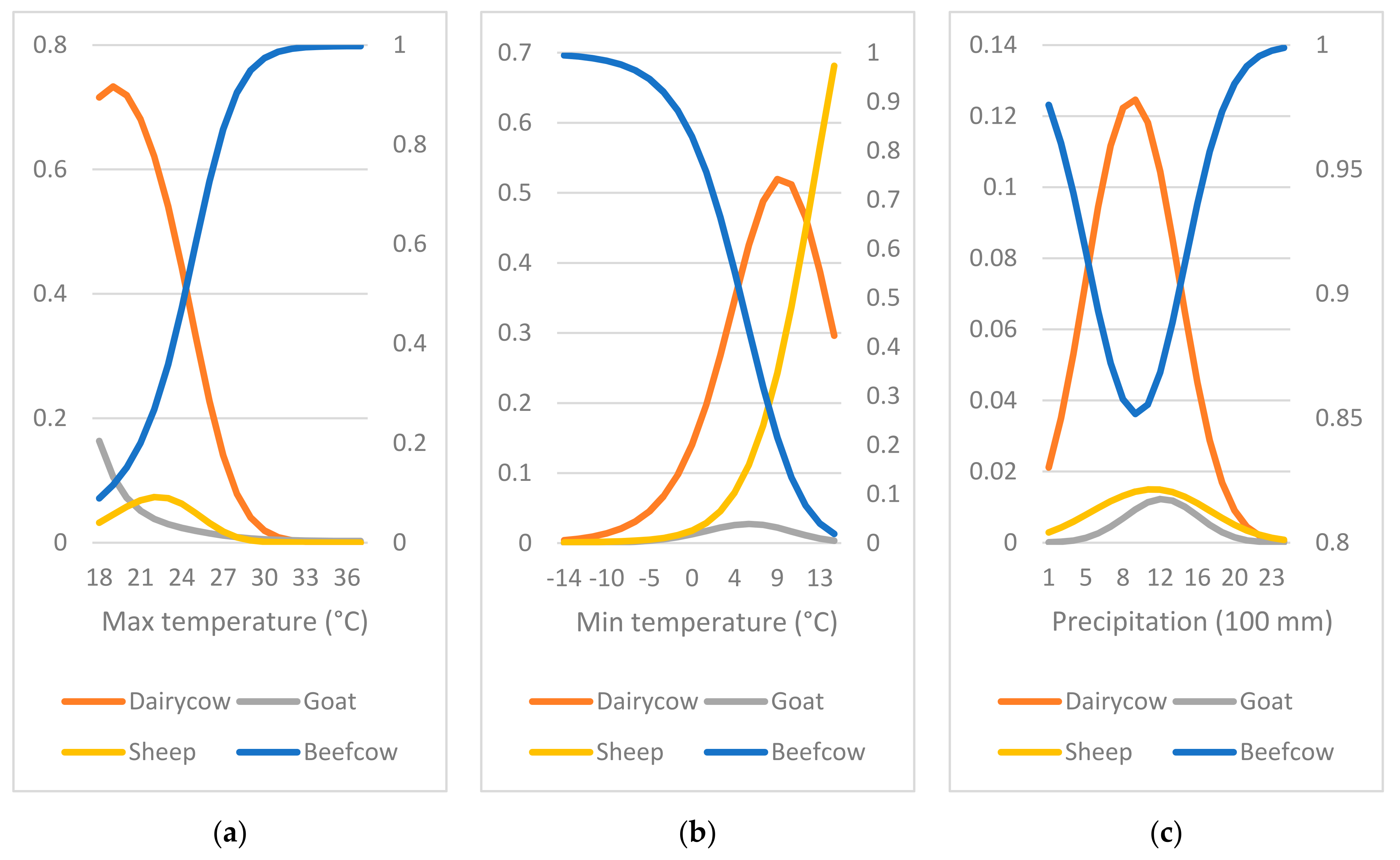
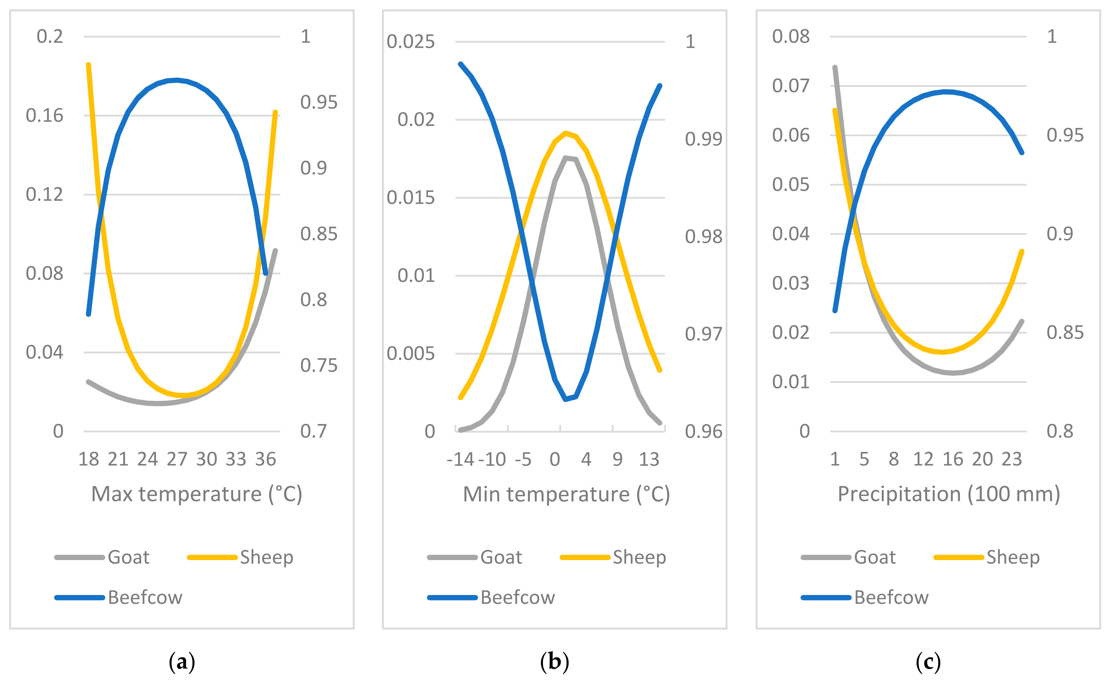
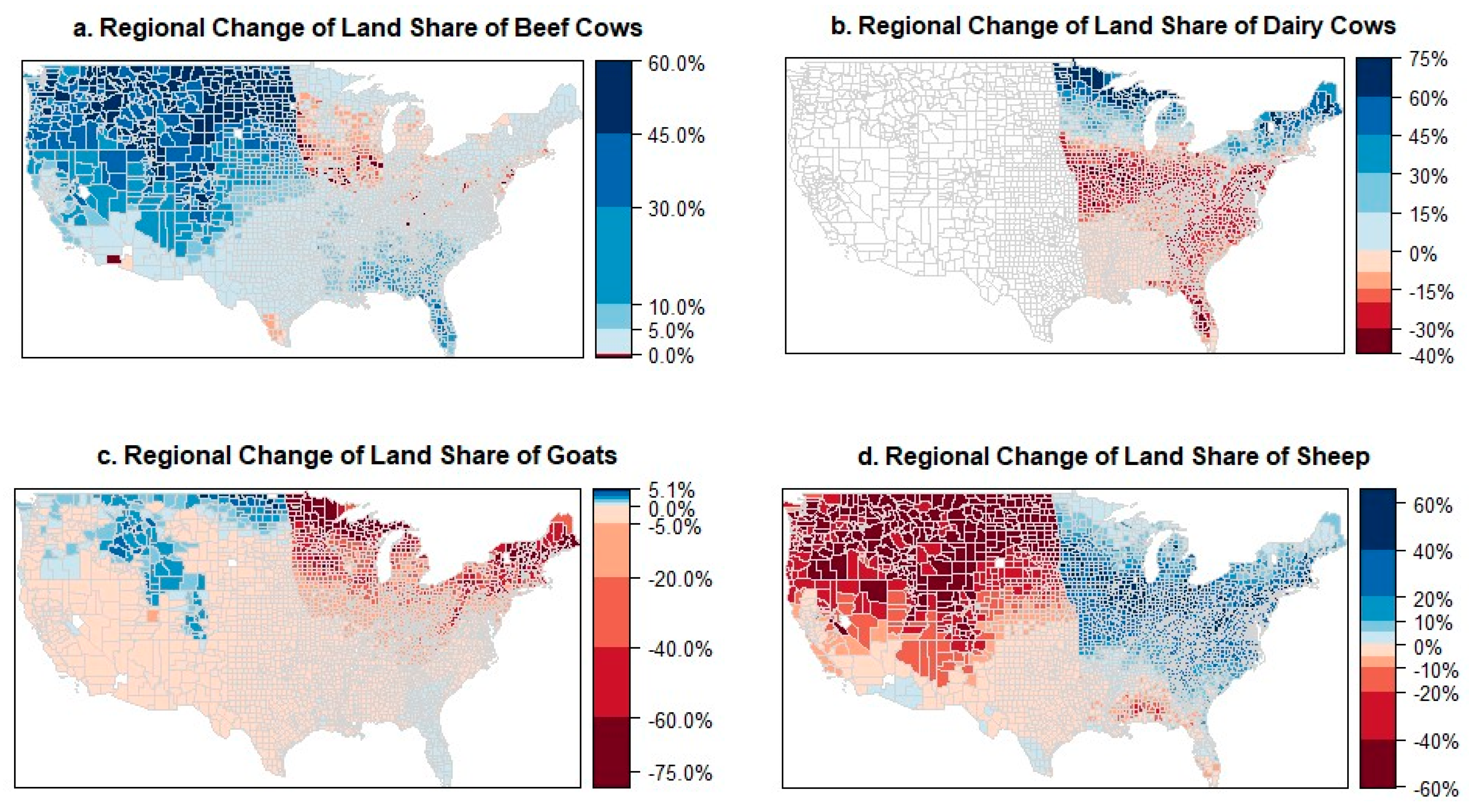
4.1. Livestock Species Mix
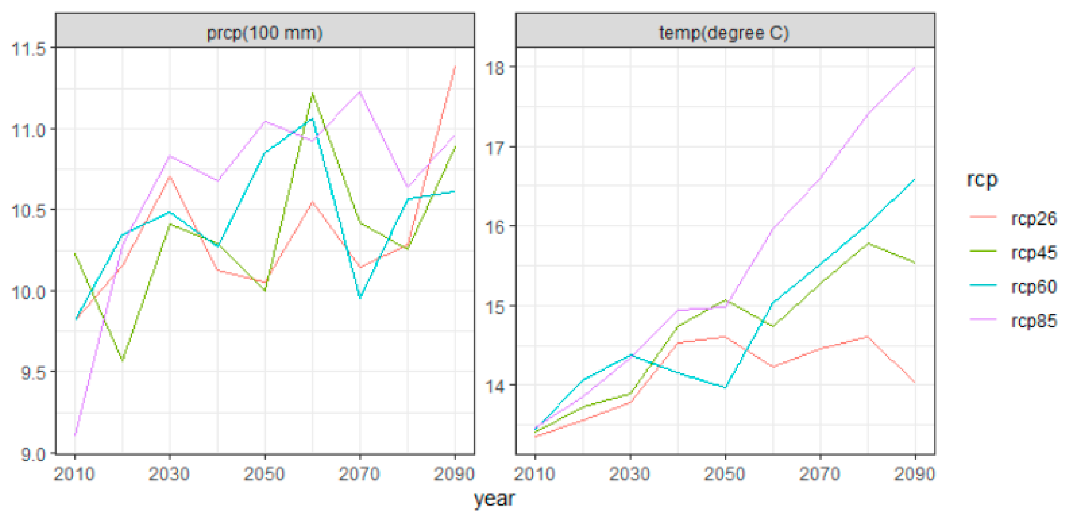
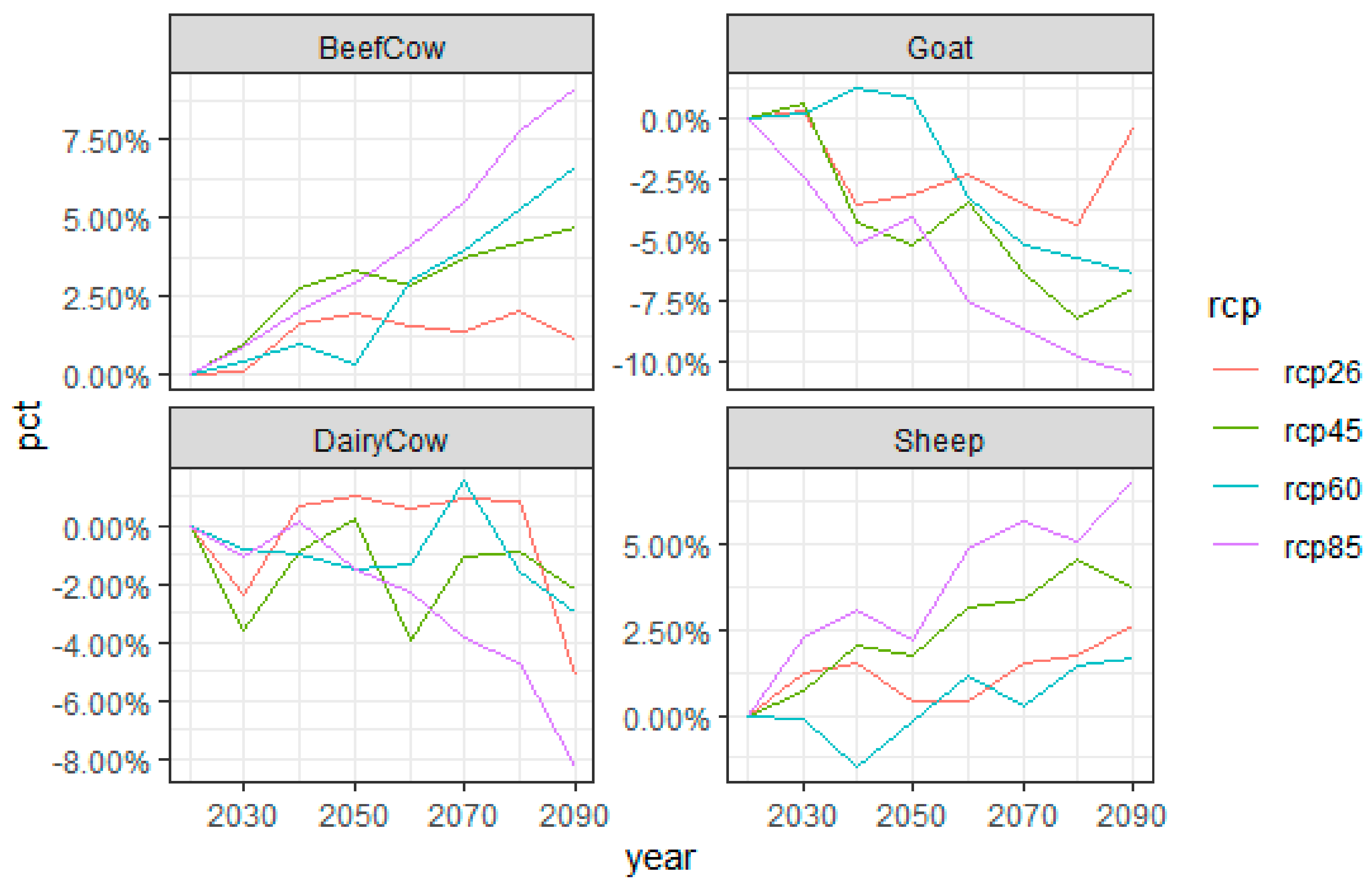
4.2. Climate Scenarios
5. Conclusions
Author Contributions
Funding
Institutional Review Board Statement
Informed Consent Statement
Data Availability Statement
Conflicts of Interest
Appendix A

| VARIABLES | Dairy Cows | Goats | Sheep |
|---|---|---|---|
| annual_tmax | 0.6183 *** | −1.3994 *** | 1.8614 *** |
| (0.2014) | (0.3438) | (0.2810) | |
| annual_tmaxsq | −0.0238 *** | 0.0194 *** | −0.0493 *** |
| (0.0040) | (0.0069) | (0.0058) | |
| annual_tmin | 0.2782 *** | 0.2702 *** | 0.3547 *** |
| (0.0147) | (0.0371) | (0.0270) | |
| annual_tminsq | 0.0010 | −0.0077 *** | 0.0086 *** |
| (0.0013) | (0.0026) | (0.0019) | |
| annual_prcp | 0.4886 *** | 0.9598 *** | 0.3736 *** |
| (0.0947) | (0.1903) | (0.1224) | |
| annual_prcpsq | −0.0261 *** | −0.0396 *** | −0.0168 *** |
| (0.0041) | (0.0077) | (0.0052) | |
| Value_cattle | −0.1377 *** | 0.0560 *** | 0.1060 *** |
| (0.0128) | (0.0217) | (0.0162) | |
| Value_milkcow | 0.1070 *** | −0.0051 | −0.0070 |
| (0.0061) | (0.0126) | (0.0094) | |
| Value_goat | 0.1862 *** | 0.2120 * | 0.0966 |
| (0.0657) | (0.1136) | (0.0775) | |
| Value_sheep | 0.2469 *** | 0.1528 | 0.4406 *** |
| (0.0547) | (0.0958) | (0.0677) | |
| GrassLand | 0.0500 | −1.5575 *** | −0.9170 *** |
| (0.0395) | (0.2975) | (0.2736) | |
| Region = LS | 0.5977 *** | 0.2032 * | 0.3438 *** |
| (0.0684) | (0.1220) | (0.0824) | |
| Region = NE | 0.7395 *** | 0.7070 *** | 0.8266 *** |
| (0.0504) | (0.0878) | (0.0603) | |
| Region = SC | −0.3843 *** | 0.0447 | −0.2985 ** |
| (0.0608) | (0.1236) | (0.1518) | |
| Region = SE | −0.6774 *** | 0.6278 *** | 0.4474 *** |
| (0.0608) | (0.1231) | (0.1445) | |
| Year = 2002 | −0.2696 *** | −0.2121 * | −0.0867 |
| (0.0520) | (0.1165) | (0.0844) | |
| Year = 2007 | −0.6154 *** | −0.1672 | −0.3636 *** |
| (0.0719) | (0.1442) | (0.1171) | |
| Year = 2012 | −1.0237 *** | −0.3843 * | −0.5037 *** |
| (0.1073) | (0.2090) | (0.1709) | |
| Year = 2017 | −1.9417 *** | −0.3564 | −0.6432 *** |
| (0.1320) | (0.2485) | (0.1991) | |
| Constant | −5.2240 * | 14.2166 *** | −20.5704 *** |
| (2.7325) | (4.7980) | (3.6909) | |
| Observations | 9941 | 9941 | 9941 |
| VARIABLES | Goats | Sheep |
|---|---|---|
| annual_tmax | −0.7557 *** | −1.5047 *** |
| (0.2080) | (0.1584) | |
| annual_tmaxsq | 0.0153 *** | 0.0277 *** |
| (0.0037) | (0.0032) | |
| annual_tmin | 0.0699 ** | 0.0253 |
| (0.0314) | (0.0195) | |
| annual_tminsq | −0.0199 *** | −0.0088 *** |
| (0.0019) | (0.0015) | |
| annual_prcp | −0.2730 *** | −0.2359 *** |
| (0.0590) | (0.0381) | |
| annual_prcpsq | 0.0086 *** | 0.0082 *** |
| (0.0027) | (0.0017) | |
| Value_cattle | 0.0089 | 0.0616 ** |
| (0.0362) | (0.0243) | |
| Value_goat | −0.2097 | −0.3525 ** |
| (0.1843) | (0.1435) | |
| Value_sheep | −0.1320 | 0.1141 ** |
| (0.2168) | (0.0577) | |
| GrassLand | −0.0148 | 0.0180 *** |
| (0.0097) | (0.0044) | |
| Region = PNW | 0.1490 | 0.1975 |
| (0.2740) | (0.1775) | |
| Region = PSW | −0.0287 | 0.8701 *** |
| (0.2985) | (0.1895) | |
| Region = RM | −0.2895 | 0.4385 *** |
| (0.2384) | (0.1278) | |
| Region = SW | −0.1887 | −0.6635 *** |
| (0.2492) | (0.1495) | |
| Year = 2002 | −0.2117 | −0.2974 *** |
| (0.1659) | (0.1072) | |
| Year = 2007 | −0.0803 | −0.4100 *** |
| (0.1803) | (0.1203) | |
| Year = 2012 | −0.3573 | −0.7970 *** |
| (0.2418) | (0.1619) | |
| Year = 2017 | −0.0330 | −0.6097 *** |
| (0.2218) | (0.1590) | |
| Constant | 7.9269 ** | 18.6982 *** |
| (3.1065) | (2.0474) | |
| Observations | 5268 | 5268 |
References
- Masson-Delmotte, V.; Zhai, P.; Pirani, P.; Connors, S.L.; Péan, C.; Berger, S.; Caud, N.; Chen, Y.; Goldfarb, L.; Gomis, M.I.; et al. IPCC, 2021: Climate Change 2021: The Physical Science Basis. Contribution of Working Group I to the Sixth Assessment Report of the Intergovernmental Panel on Climate Change; Cambridge University Press: Cambridge, UK, 2021; in press. [Google Scholar]
- Shukla, P.R.; Skea, J.; Calvo Buendia, E.; Masson-Delmotte, V.; Pörtner, H.O.; Roberts, D.C.; Zhai, P.; Slade, R.; Connors, S.; Van Diemen, R. IPCC, 2019: Climate Change and Land: An IPCC Special Report on Climate Change, Desertification, Land Degradation, Sustainable Land Management, Food Security, and Greenhouse Gas Fluxes in Terrestrial Ecosystems; Intergovernmental Panel on Climate Change (IPCC): Geneva, Switzerland, 2019. [Google Scholar]
- Mendelsohn, R.O.; Nordhaus, W.D.; Shaw, D. The Impact of Global Warming on Agriculture: A Ricardian Analysis. Am. Econ. Rev. 1994, 84, 753–771. [Google Scholar]
- USDA. 2017 Census of Agriculture Highlights; US Department of Agriculture: Washington, DC, USA, 2017.
- USDA. 2017 Census of Agriculture; US Department of Agriculture: Washington, DC, USA, 2019.
- Roenfeldt, S. You Can’t Afford to Ignore Heat Stress. Dairy Herd Manag. 1998, 35, 6–12. [Google Scholar]
- Hristov, A.N.; DeGaetano, A.T.; Rotz, C.A.; Hoberg, E.; Skinner, R.H.; Felix, T.; Li, H.; Patterson, P.H.; Roth, G.; Hall, M.; et al. Climate change effects on livestock in the Northeast US and strategies for adaptation. Clim. Chang. 2017, 146, 33–45. [Google Scholar] [CrossRef] [Green Version]
- St-Pierre, N.; Cobanov, B.; Schnitkey, G. Economic Losses from Heat Stress by US Livestock Industries. J. Dairy Sci. 2003, 86, E52–E77. [Google Scholar] [CrossRef] [Green Version]
- Nienaber, J.; Hahn, G. Livestock production system management responses to thermal challenges. Int. J. Biometeorol. 2007, 52, 149–157. [Google Scholar] [CrossRef] [Green Version]
- Sejian, V.; Maurya, V.P.; Kumar, K.; Naqvi, S.M.K. Effect of multiple stresses on growth and adaptive capability of Malpura ewes under semi-arid tropical environment. Trop. Anim. Health Prod. 2012, 45, 107–116. [Google Scholar] [CrossRef]
- Nardone, A.; Ronchi, B.; Lacetera, N.; Ranieri, M.; Bernabucci, U. Effects of climate changes on animal production and sustainability of livestock systems. Livest. Sci. 2010, 130, 57–69. [Google Scholar] [CrossRef]
- Intergovernmental Panel on Climate Change. Climate Change 2014: Impacts, Adaptation, and Vulnerability-Part B: Regional Aspects-Contribution of Working Group II to the Fifth Assessment Report of the Intergovernmental Panel on Climate Change; Barros, V.R., Field, C.B., Dokken, D.J., Mastrandrea, M.D., Mach, K.J., Bilir, T.E., Chatterjee, M., Ebi, K.L., Estrada, Y.O., Genova, R.C., et al., Eds.; Cambridge University Press: Cambridge, UK; New York, NY, USA, 2014; ISBN 978-1-107-68386-0. [Google Scholar]
- Intergovernmental Panel on Climate Change. Climate Change 2001: Impacts, Adaptation and Vulnerability. Contribution of Working Group II to the Third Assessment Report of the Intergovernmental Panel on Climate Change; Cambridge University Press: Cambridge, UK, 2001. [Google Scholar]
- Herrero, M.; Thornton, P.; Kruska, R.; Reid, R. Systems dynamics and the spatial distribution of methane emissions from African domestic ruminants to 2030. Agric. Ecosyst. Environ. 2008, 126, 122–137. [Google Scholar] [CrossRef]
- Hoffmann, I. Climate change and the characterization, breeding and conservation of animal genetic resources. Anim. Genet. 2010, 41, 32–46. [Google Scholar] [CrossRef]
- Mu, J.E.; McCarl, B.A.; Wein, A.M. Adaptation to climate change: Changes in farmland use and stocking rate in the U.S. Mitig. Adapt. Strat. Glob. Chang. 2013, 18, 713–730. [Google Scholar] [CrossRef] [Green Version]
- Zhang, Y.W.; Hagerman, A.D.; McCarl, B.A. Influence of climate factors on spatial distribution of Texas cattle breeds. Clim. Chang. 2013, 118, 183–195. [Google Scholar] [CrossRef]
- Cho, S.J.; McCarl, B.A. Climate change influences on crop mix shifts in the United States. Sci. Rep. 2017, 7, 40845. [Google Scholar] [CrossRef] [Green Version]
- Seo, S.N.; Mendelsohn, R.O. Measuring Impacts and Adaptations to Climate Change: A Structural Ricardian Model of African Livestock Management. Agric. Econ. 2008, 38, 151–165. [Google Scholar] [CrossRef]
- Tubiello, F.; Rosenzweig, C.; Goldberg, R.; Jagtap, S.; Jones, J. Effects of climate change on US crop production: Simulation results using two different GCM scenarios. Part I: Wheat, potato, maize, and citrus. Clim. Res. 2002, 20, 259–270. [Google Scholar] [CrossRef] [Green Version]
- Ovalle-Rivera, O.; Läderach, P.; Bunn, C.; Obersteiner, M.; Schroth, G. Projected Shifts in Coffea arabica Suitability among Major Global Producing Regions Due to Climate Change. PLoS ONE 2015, 10, e0124155. [Google Scholar] [CrossRef] [Green Version]
- Hijmans, R.J. The effect of climate change on global potato production. Am. J. Potato Res. 2003, 80, 271–279. [Google Scholar] [CrossRef]
- Machovina, B.; Feeley, K.J. Climate change driven shifts in the extent and location of areas suitable for export banana production. Ecol. Econ. 2013, 95, 83–95. [Google Scholar] [CrossRef]
- Havlík, P.; Valin, H.; Mosnier, A.; Obersteiner, M.; Baker, J.S.; Herrero, M.; Rufino, M.C.; Schmid, E. Crop Productivity and the Global Livestock Sector: Implications for Land Use Change and Greenhouse Gas Emissions. Am. J. Agric. Econ. 2012, 95, 442–448. [Google Scholar] [CrossRef]
- Mu, J.E.; Sleeter, B.M.; Abatzoglou, J.T.; Antle, J.M. Climate impacts on agricultural land use in the USA: The role of socio-economic scenarios. Clim. Chang. 2017, 144, 329–345. [Google Scholar] [CrossRef] [Green Version]
- Ghahramani, A.; Kingwell, R.; Maraseni, T.N. Land use change in Australian mixed crop-livestock systems as a transformative climate change adaptation. Agric. Syst. 2020, 180, 102791. [Google Scholar] [CrossRef]
- Mu, J.E.; McCarl, B.A.; Sleeter, B.; Abatzoglou, J.T.; Zhang, H. Adaptation with climate uncertainty: An examination of agricultural land use in the United States. Land Use Policy 2018, 77, 392–401. [Google Scholar] [CrossRef]
- Kabubo-Mariara, J. Climate change adaptation and livestock activity choices in Kenya: An economic analysis. Nat. Resour. Forum 2008, 32, 131–141. [Google Scholar] [CrossRef]
- Seo, S.N.; McCarl, B.A.; Mendelsohn, R. From beef cattle to sheep under global warming? An analysis of adaptation by livestock species choice in South America. Ecol. Econ. 2010, 69, 2486–2494. [Google Scholar] [CrossRef]
- Mader, T.L.; Frank, K.L.; Harrington, J.A., Jr.; Hahn, L.G.; Nienaber, J.A. Potential climate change effects on warm-season livestock production in the Great Plains. Clim. Chang. 2009, 97, 529–541. [Google Scholar] [CrossRef] [Green Version]
- Craine, J.M.; Elmore, A.; Olson, K.C.; Tolleson, D. Climate change and cattle nutritional stress. Glob. Chang. Biol. 2010, 16, 2901–2911. [Google Scholar] [CrossRef]
- Hahn, G.L. Dynamic responses of cattle to thermal heat loads. J. Anim. Sci. 1997, 77, 10–20. [Google Scholar] [CrossRef]
- Seo, S.N.; McCarl, B. Managing Livestock Species under Climate Change in Australia. Animals 2011, 1, 343–365. [Google Scholar] [CrossRef] [Green Version]
- Seo, S.N. Adapting to extreme climates: Raising animals in hot and arid ecosystems in Australia. Int. J. Biometeorol. 2014, 59, 541–550. [Google Scholar] [CrossRef] [PubMed]
- Godde, C.; Dizyee, K.; Ash, A.; Thornton, P.; Sloat, L.; Roura, E.; Henderson, B.; Herrero, M. Climate change and variability impacts on grazing herds: Insights from a system dynamics approach for semi-arid Australian rangelands. Glob. Chang. Biol. 2019, 25, 3091–3109. [Google Scholar] [CrossRef] [Green Version]
- Schlenker, W.; Hanemann, W.M.; Fisher, A.C. The Impact of Global Warming on U.S. Agriculture: An Econometric Analysis of Optimal Growing Conditions. Rev. Econ. Stat. 2006, 88, 113–125. [Google Scholar] [CrossRef]
- Redfearn, D.D.; Bidwell, T.G. Stocking Rate: The Key to Successful Livestock Production. 2006. Available online: https://extension.okstate.edu/fact-sheets/print-publications/pss/stocking-rate-the-key-to-successful-livestock-production-pss-2871.pdf (accessed on 17 November 2021).
- Adams, D.M.; Alig, R.J.; McCarl, B.A.; Murray, B.C. FASOMGHG Conceptual Structure, and Specification: Documentation 2005. Available online: https://docplayer.net/62907502-Fasomghg-conceptual-structure-and-specification-documentation.html (accessed on 17 November 2021).
- Mullahy, J. Multivariate Fractional Regression Estimation of Econometric Share Models. J. Econ. Methods 2015, 4, 71–100. [Google Scholar] [CrossRef]
- Murteira, J.M.R.; Ramalho, J. Regression Analysis of Multivariate Fractional Data. Econ. Rev. 2014, 35, 515–552. [Google Scholar] [CrossRef]
- Ramalho, E.A.; Ramalho, J.J.S.; Murteira, J.M.R. Alternative Estimating and Testing Empirical Strategies for Fractional Regression Models. J. Econ. Surv. 2011, 25, 19–68. [Google Scholar] [CrossRef]
- Papke, L.E.; Wooldridge, J.M. Econometric Methods for Fractional Response Variables with an Application to 401(K) Plan Participation Rates. J. Appl. Econom. 1996, 11, 619–632. [Google Scholar] [CrossRef] [Green Version]
- Long, J.S.; Freese, J. Regression Models for Categorical Dependent Variables Using Stata; Stata Press: College Station, TX, USA, 2006; Volume 7. [Google Scholar]
- Fisher, A.C.; Hanemann, W.M.; Roberts, M.J.; Schlenker, W. The Economic Impacts of Climate Change: Evidence from Agricultural Output and Random Fluctuations in Weather: Comment. Am. Econ. Rev. 2012, 102, 3749–3760. [Google Scholar] [CrossRef]
- USDA’s Economic Research Service USDA ERS Farm Resource Regions. Available online: https://www.ers.usda.gov/webdocs/publications/42298/32489_aib-760_002.pdf?v=42487 (accessed on 23 October 2021).
- US Department of Agriculture. Quick Stats 2.0; National Agricultural Statistics Service, US Department of Agriculture: Washington, DC, USA, 2018.
- Menne, M.J.; Durre, I.; Vose, R.S.; Gleason, B.E.; Houston, T.G. An Overview of the Global Historical Climatology Network-Daily Database. J. Atmos. Ocean. Technol. 2012, 29, 897–910. [Google Scholar] [CrossRef]
- USDA’s Economic Research Service Milk Cost of Production Estimates. Available online: https://www.ers.usda.gov/data-products/milk-cost-of-production-estimates/ (accessed on 21 August 2021).
- USDA. Land Values 2021 Summary; US Department of Agriculture: Washington, DC, USA, 2021; p. 22.
- US Department of the Interior, Bureau of Reclamation, Technical Services Center. Downscaled CMIP3 and CMIP5 Climate and Hydrology Projections: Release of Downscaled CMIP5 Climate Projections, Comparison with Preceding Information, and Summary of User Needs; US Department of the Interior Denver: Lakewood, CO, USA, 2013; p. 47.


| Hypotheses | Reasoning |
|---|---|
| 1. The share of each livestock species has a nonlinear relationship with climate factors. | Animals have optimal temperature ranges for growth and comfort known as the thermoneutral zone (TNZ). Livestock yield the highest productivity within the TNZ but may lose profitability if the climate falls above or below that zone. Thus, the share of each species is affected by climate factors. |
| 2. Magnitudes of sensitivity to climate vary by species. | Different species have different TNZs, and their land use shifts differentially under altered environmental factors. For example, dairy cows’ milk yields may drop significantly under hot and wet conditions while goats are more heat tolerant. |
| 3. Livestock share locations will shift under climate change. | With climate change, the climate of some regions may become favorable for a specific species while that of others may become likely to cause greater heat stress or cold stress. Local farmers will adapt to climate change by changing species land use shares. |
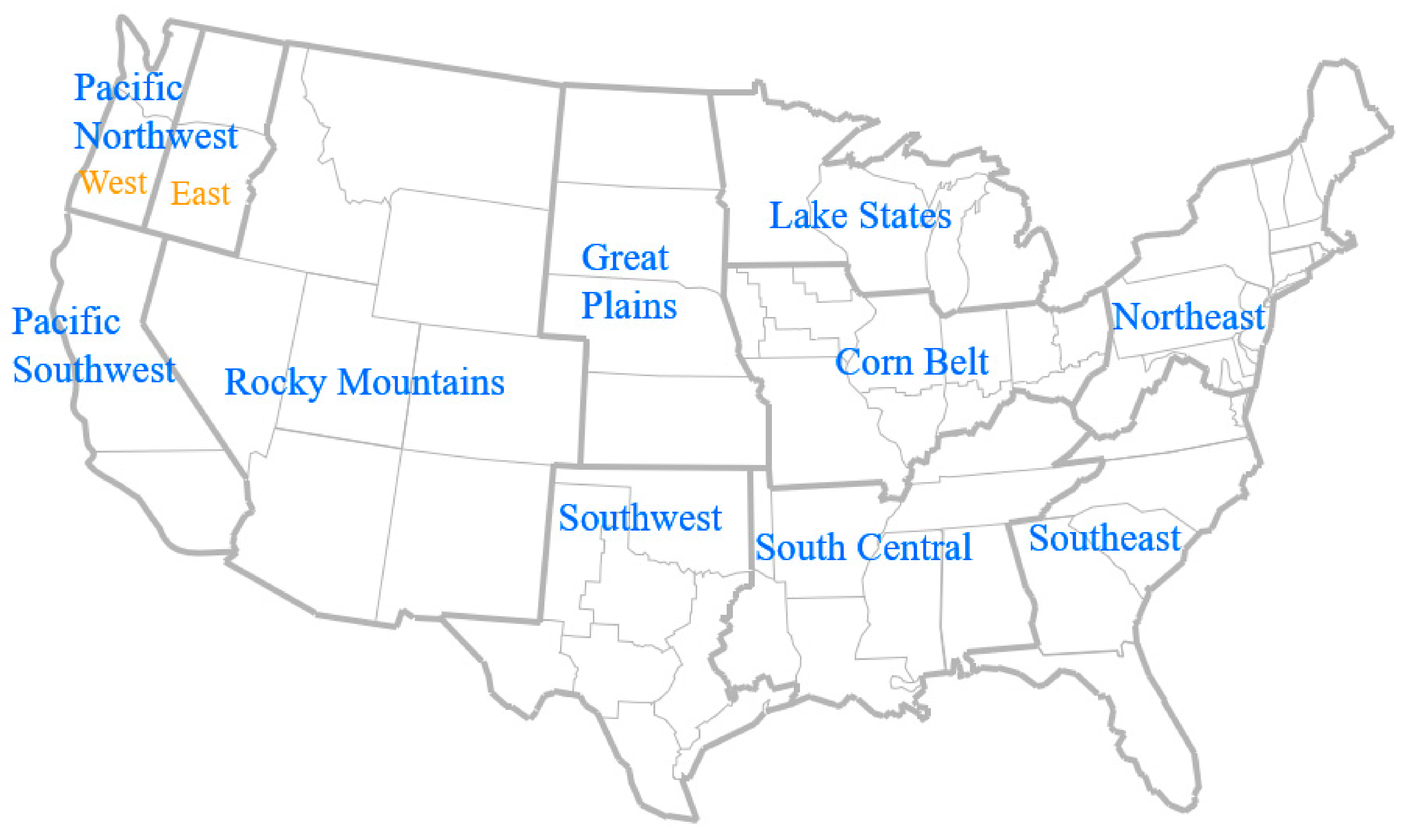
| Region | Market Region | States | |
|---|---|---|---|
| East | Corn Belt | CB | IL, IN, IA, MO, OH |
| Lake States | LS | MI, MN, WI | |
| Northeast | NE | CT, DE, ME, MD, MA, NH, NJ, NY, PA, RI, VT, WV | |
| South Central | SC | AL, AR, KY, LA, MS, TN | |
| Southeast | SE | FL, GA, NC, SC, VA | |
| West | Great Plains | GP | KS, NE, ND, SD |
| Pacific Northwest | PNW | OR, WA | |
| Pacific Southwest | PSW | CA | |
| Rocky Mountains | RM | AZ, CO, ID, MT, NV, NM, UT, WY | |
| Southwest | SW | OK, TX |
| Region | Market Region | Beef Cow | Dairy Cow | Goat | Sheep |
|---|---|---|---|---|---|
| East | CB | 75.36% | 19.05% | 1.86% | 3.73% |
| LS | 39.80% | 53.76% | 1.94% | 4.50% | |
| NE | 42.29% | 46.03% | 4.07% | 7.61% | |
| SC | 92.64% | 4.08% | 2.22% | 1.05% | |
| SE | 83.25% | 8.09% | 5.60% | 3.05% | |
| Total | 72.53% | 20.87% | 3.13% | 3.47% | |
| West | GP | 94.56% | 0.00% | 1.54% | 3.90% |
| PNW | 89.81% | 0.00% | 2.50% | 7.68% | |
| PSW | 84.18% | 0.00% | 3.64% | 12.18% | |
| RM | 88.62% | 0.00% | 1.98% | 9.40% | |
| SW | 92.55% | 0.00% | 4.04% | 3.41% | |
| Total | 91.52% | 0.00% | 2.56% | 5.91% |
| Variable | Explanation | Unit | N | Mean | St. Dev. | Min | Max |
|---|---|---|---|---|---|---|---|
| annual_prcp | 3-year moving average of annual temperature and precipitation and their squares | 100 mm | 15,240 | 9.81 | 3.48 | 0.80 | 24.68 |
| annual_tmax | °C | 15,240 | 26.70 | 3.42 | 17.57 | 36.52 | |
| annual_tmin | °C | 15,240 | −0.95 | 4.93 | −14.38 | 15.26 | |
| annual_prcpsq | °C2 | 15,240 | 108.76 | 65.52 | 0.64 | 609.16 | |
| annual_tmaxsq | °C2 | 15,240 | 724.34 | 180.05 | 308.83 | 1334.03 | |
| annual_tminsq | 10,000 mm2 | 15,240 | 25.18 | 31.67 | 0.00 | 233.00 | |
| Value_beefcow | The market value per unit of livestock | USD | 15,240 | 678.97 | 246.35 | 152.12 | 2080.00 |
| Value_dairycow | USD | 15,240 | 2927.30 | 811.09 | 1602.22 | 4875.65 | |
| Value_goat | USD | 15,240 | 132.04 | 25.62 | 6.91 | 891.35 | |
| Value_sheep | USD | 15,240 | 161.60 | 30.83 | 56.29 | 1816.87 | |
| Grassland | Grassland available | 1000 acres | 15,240 | 151.69 | 335.25 | 0.02 | 6151.50 |
| Region | Regional dummies | NA | 15,240 | NA | NA | 0.00 | 1.00 |
| Year | Year dummies | NA | 15,240 | NA | NA | 0.00 | 1.00 |
| East | West | |||||||||||
|---|---|---|---|---|---|---|---|---|---|---|---|---|
| Variable | CB | LS | NE | SC | SE | Total | GP | PNW | PSW | RM | SW | Total |
| annual_prcp | 10.38 | 8.35 | 11.48 | 13.48 | 12.37 | 11.54 | 6.41 | 9.81 | 6.15 | 3.71 | 8.39 | 6.55 |
| annual_tmax | 25.39 | 21.3 | 24.09 | 28.58 | 28.88 | 26.33 | 26.03 | 22.59 | 28.77 | 25.09 | 31.49 | 27.4 |
| annual_tmin | −2.86 | −6.93 | −3.11 | 2.38 | 3.73 | −0.53 | −5.82 | −1.12 | 3.89 | −5.36 | 3.86 | −1.81 |
| Value_cattle | 7.7 | 7.32 | 6.04 | 5.68 | 5.52 | 6.4 | 8.86 | 7 | 6.97 | 7.13 | 6.82 | 7.53 |
| Value_milkcow | 28.77 | 31.37 | 29.58 | 23.68 | 31.31 | 28.52 | 29.1 | 33.67 | 31.41 | 32.03 | 30.33 | 30.7 |
| Value_goat | 1.38 | 1.46 | 1.43 | 1.19 | 1.23 | 1.31 | 1.33 | 1.44 | 1.53 | 1.34 | 1.28 | 1.34 |
| Value_sheep | 1.64 | 1.66 | 1.68 | 1.47 | 1.57 | 1.59 | 1.69 | 1.76 | 1.89 | 1.74 | 1.52 | 1.66 |
| Grassland | 3.58 | 2.12 | 1.72 | 4.31 | 2.92 | 3.16 | 23.60 | 23.39 | 26.47 | 63.66 | 36.94 | 38.37 |
| VARIABLES | Beef Cows | Dairy Cows | Goats | Sheep |
|---|---|---|---|---|
| annual_tmax | −0.0729 *** | 0.0639 *** | −0.0471 *** | 0.0562 *** |
| (0.0265) | (0.0238) | (0.0102) | (0.0090) | |
| annual_tmaxsq | 0.0031 *** | −0.0025 *** | 0.0008 *** | −0.0014 *** |
| (0.0005) | (0.0005) | (0.0002) | (0.0002) | |
| annual_tmin | −0.0428 *** | 0.0286 *** | 0.0059 *** | 0.0083 *** |
| (0.0020) | (0.0018) | (0.0011) | (0.0009) | |
| annual_tminsq | −0.0001 | 0.0001 | −0.0002 *** | 0.0003 *** |
| (0.0002) | (0.0002) | (0.0001) | (0.0001) | |
| annual_prcp | −0.0807 *** | 0.0500 *** | 0.0249 *** | 0.0059 |
| (0.0119) | (0.0114) | (0.0056) | (0.0040) | |
| annual_prcpsq | 0.0040 *** | −0.0028 *** | −0.0010 *** | −0.0002 |
| (0.0005) | (0.0005) | (0.0002) | (0.0002) | |
| Value_beefcow | 0.0110 *** | −0.0182 *** | 0.0023 *** | 0.0048 *** |
| (0.0016) | (0.0015) | (0.0006) | (0.0005) | |
| Value_milkcow | −0.0110 *** | 0.0131 *** | −0.0008 ** | −0.0013 *** |
| (0.0008) | (0.0007) | (0.0004) | (0.0003) | |
| Value_goat | −0.0264 *** | 0.0204 *** | 0.0050 | 0.0009 |
| (0.0091) | (0.0075) | (0.0032) | (0.0022) | |
| Value_sheep | −0.0387 *** | 0.0245 *** | 0.0025 | 0.0116 *** |
| (0.0073) | (0.0064) | (0.0027) | (0.0020) | |
| Grassland | 0.0487 *** | 0.0248 *** | −0.0449 *** | −0.0285 *** |
| (0.0117) | (0.0061) | (0.0087) | (0.0087) | |
| Region = LS | −0.0912 *** | 0.0859 *** | 0.0010 | 0.0044 * |
| (0.0110) | (0.0112) | (0.0028) | (0.0026) | |
| Region = NE | −0.1327 *** | 0.0989 *** | 0.0136 *** | 0.0201 *** |
| (0.0081) | (0.0082) | (0.0026) | (0.0024) | |
| Region = SC | 0.0476 *** | −0.0455 *** | 0.0030 | −0.0052 |
| (0.0082) | (0.0074) | (0.0029) | (0.0036) | |
| Region = SE | 0.0395 *** | −0.0827 *** | 0.0227 *** | 0.0205 *** |
| (0.0093) | (0.0066) | (0.0043) | (0.0060) | |
| Year = 2002 | 0.0388 *** | −0.0358 *** | −0.0040 | 0.0009 |
| (0.0076) | (0.0075) | (0.0034) | (0.0028) | |
| Year = 2007 | 0.0825 *** | −0.0783 *** | −0.0002 | −0.0040 |
| (0.0100) | (0.0101) | (0.0042) | (0.0037) | |
| Year = 2012 | 0.1315 *** | −0.1235 *** | −0.0039 | −0.0041 |
| (0.0138) | (0.0137) | (0.0058) | (0.0053) | |
| Year = 2017 | 0.2059 *** | −0.2051 *** | 0.0010 | −0.0017 |
| (0.0148) | (0.0136) | (0.0073) | (0.0061) | |
| Observations | 9941 | 9941 | 9941 | 9941 |
| VARIABLES | Beef Cows | Goats | Sheep |
|---|---|---|---|
| annual_tmax | 0.0952 *** | −0.0159 *** | −0.0794 *** |
| (0.0113) | (0.0049) | (0.0086) | |
| annual_tmaxsq | −0.0018 *** | 0.0003 *** | 0.0015 *** |
| (0.0002) | (0.0001) | (0.0002) | |
| annual_tmin | −0.0029 ** | 0.0017 ** | 0.0012 |
| (0.0015) | (0.0007) | (0.0010) | |
| annual_tminsq | 0.0009 *** | −0.0005 *** | −0.0004 *** |
| (0.0001) | (0.0001) | (0.0001) | |
| annual_prcp | 0.0185 *** | −0.0063 *** | −0.0122 *** |
| (0.0029) | (0.0015) | (0.0020) | |
| annual_prcpsq | −0.0006 *** | 0.0002 *** | 0.0004 *** |
| (0.0001) | (0.0001) | (0.0001) | |
| Value_beefcow | −0.0034 * | 0.0001 | 0.0033 ** |
| (0.0018) | (0.0009) | (0.0013) | |
| Value_goat | 0.0231 ** | −0.0045 | −0.0185 ** |
| (0.0101) | (0.0044) | (0.0076) | |
| Value_sheep | −0.0029 | −0.0034 | 0.0064 ** |
| (0.0064) | (0.0053) | (0.0030) | |
| Grassland | −0.0006 | −0.0004 * | 0.0010 *** |
| (0.0004) | (0.0002) | (0.0002) | |
| Region = PNW | −0.0146 | 0.0039 | 0.0107 |
| (0.0142) | (0.0080) | (0.0100) | |
| Region = PSW | −0.0619 *** | −0.0034 | 0.0653 *** |
| (0.0195) | (0.0077) | (0.0159) | |
| Region = RM | −0.0201 * | −0.0080 | 0.0281 *** |
| (0.0106) | (0.0060) | (0.0077) | |
| Region = SW | 0.0296 *** | −0.0039 | −0.0257 *** |
| (0.0100) | (0.0066) | (0.0061) | |
| Year = 2002 | 0.0242 ** | −0.0046 | −0.0196 *** |
| (0.0095) | (0.0041) | (0.0074) | |
| Year = 2007 | 0.0275 *** | −0.0012 | −0.0263 *** |
| (0.0105) | (0.0047) | (0.0082) | |
| Year = 2012 | 0.0510 *** | −0.0070 | −0.0440 *** |
| (0.0125) | (0.0057) | (0.0096) | |
| Year = 2017 | 0.0360 *** | 0.0005 | −0.0365 *** |
| (0.0129) | (0.0059) | (0.0098) | |
| Observations | 5268 | 5268 | 5268 |
Publisher’s Note: MDPI stays neutral with regard to jurisdictional claims in published maps and institutional affiliations. |
© 2021 by the authors. Licensee MDPI, Basel, Switzerland. This article is an open access article distributed under the terms and conditions of the Creative Commons Attribution (CC BY) license (https://creativecommons.org/licenses/by/4.0/).
Share and Cite
Wang, M.; McCarl, B.A. Impacts of Climate Change on Livestock Location in the US: A Statistical Analysis. Land 2021, 10, 1260. https://doi.org/10.3390/land10111260
Wang M, McCarl BA. Impacts of Climate Change on Livestock Location in the US: A Statistical Analysis. Land. 2021; 10(11):1260. https://doi.org/10.3390/land10111260
Chicago/Turabian StyleWang, Minglu, and Bruce A. McCarl. 2021. "Impacts of Climate Change on Livestock Location in the US: A Statistical Analysis" Land 10, no. 11: 1260. https://doi.org/10.3390/land10111260
APA StyleWang, M., & McCarl, B. A. (2021). Impacts of Climate Change on Livestock Location in the US: A Statistical Analysis. Land, 10(11), 1260. https://doi.org/10.3390/land10111260