Article

Remote Sensing-Based Estimation of Advanced Perennial Grass Biomass Yields for Bioenergy

1
Argonne National Laboratory, Environmental Science Division, 9700 South Cass Avenue, Lemont, IL 60439, USA
2
Crop Science Department, University of Illinois Urbana-Champaign, 1102 S Goodwin Avenue, Urbana, IL 61801, USA
3
Department of Agronomy, Horticulture, and Plant Science, South Dakota State University, Box-2140C University Station, Brookings, SD 57007, USA
4
Department of Agronomy, Iowa State University, 1223 Agronomy Hall, Ames, IA 50011, USA
5
USDA-ARS Wheat, Sorghum, and Forage Research Unit, 251 Filley Hall, East Campus, University of Nebraska-Lincoln, Lincoln, NE 68583, USA
*
Author to whom correspondence should be addressed.
Land 2021, 10(11), 1221; https://doi.org/10.3390/land10111221
Submission received: 8 October 2021 / Revised: 30 October 2021 / Accepted: 3 November 2021 / Published: 10 November 2021
(This article belongs to the Special Issue Remote Sensing Analysis of Agricultural Landscapes)

Abstract

:
A sustainable bioeconomy would require growing high-yielding bioenergy crops on marginal agricultural areas with minimal inputs. To determine the cost competitiveness and environmental sustainability of such production systems, reliably estimating biomass yield is critical. However, because marginal areas are often small and spread across the landscape, yield estimation using traditional approaches is costly and time-consuming. This paper demonstrates the (1) initial investigation of optical remote sensing for predicting perennial bioenergy grass yields at harvest using a linear regression model with the green normalized difference vegetation index (GNDVI) derived from Sentinel-2 imagery and (2) evaluation of the model’s performance using data from five U.S. Midwest field sites. The linear regression model using midsummer GNDVI predicted yields at harvest with R2 as high as 0.879 and a mean absolute error and root mean squared error as low as 0.539 Mg/ha and 0.616 Mg/ha, respectively, except for the establishment year. Perennial bioenergy grass yields may be predicted 152 days before the harvest date on average, except for the establishment year. The green spectral band showed a greater contribution for predicting yields than the red band, which is indicative of increased chlorophyll content during the early growing season. Although additional testing is warranted, this study showed a great promise for a remote sensing approach for forecasting perennial bioenergy grass yields to support critical economic and logistical decisions of bioeconomy stakeholders.

1. Introduction

Global efforts on the adoption of a biomass-based economy are increasing, particularly in the European Union and the United States (U.S.), to significantly displace our dependence on fossil-based energy and products in the coming decade [1]. For instance, in the U.S., the Biomass Research and Development (BRD) Act of 2000 [2] has paved the way for the Bioeconomy Initiative, a concerted, inter–federal agency effort that started in 2013, which is geared towards maximizing the utilization of the nation’s abundant biomass resources for bioenergy and biobased products [3]. In 2014, the biobased products sector had contributed USD 393 billion and 4.2 million jobs to the U.S. economy [4]. As the market for bioproducts (renewable biochemicals and biopolymers) and bioenergy grows, the demand for biomass is expected to increase significantly in the coming decades. The U.S. has the potential to produce at least 1 billion dry tons of biomass annually from a wide range of sources, including agricultural and forest residues, dedicated energy crops, algae, and municipal solid wastes by 2040 [5]. Dedicated energy crops, along with algae and additional waste streams, are expected to become a major source of biomass for a thriving future bioeconomy. The large-scale production of dedicated bioenergy crops in agricultural landscapes needs to be done both cost-effectively and sustainably in order to meet the 1-billion-ton goal in the U.S. [6,7]. Improved economic and production sustainability can, in part, be addressed by the selection of advanced bioenergy crop cultivars that have increased yields yet lower requirements for water and nutrient inputs relative to traditional row crops [7]. However, a major sustainability challenge of large-scale, monocultural production systems for bioenergy crops is the associated indirect land-use change that may compete for land allocated for food, feed, and fiber production [6,8]. Multifunctional landscape production systems focusing on the utilization of marginally productive agricultural lands [9,10,11,12] have been proposed to help address this concern.
A multifunctional agricultural landscape involves maximizing the productivity of the land while minimizing the input requirements and environmental impacts by strategically placing the bioenergy crops within the agricultural landscape. Placement is based on the productive capacity of the soil and/or environmental quality degradation potential [9]. In this production system, food crops will continue to be grown on fertile parts of the landscape while perennial biomass crops could be more suited in the marginal areas where row crop yields are historically low and nutrient leaching and soil erosion are prevalent [9,13]. However, marginal areas primarily comprise groups of relatively small-sized lands that are spread across the agricultural landscape [13]. Therefore, one of the challenges with this type of production strategy is the need for rapid, accurate, and cost-effective estimation of harvestable biomass yield on a small geographic scale (i.e., plot or subfield). Reliable data on biomass yield at harvest time are critical inputs for relevant meta-analyses, including technoeconomic and life-cycle greenhouse gas emission analyses, which are necessary in determining the cost competitiveness and environmental sustainability of bioenergy production systems. Rapid and large-scale assessment of biomass yield for improved cultivars may also be important to speed up cultivar evaluation and possible public release of higher-yielding and more resilient varieties for commercial production. Currently, the most common method of determining biomass yield for bioenergy grass crops is by weighing cut and baled aboveground biomass, which would be time-consuming for biomass production systems, especially at the watershed or regional scales. Although such biomass measurement would continue to be required for commercial sales transactions, the ability to estimate yields prior to harvest can assist biomass refineries and other organizations in forecasting biomass supply both locally and regionally [14,15].
Remote sensing could enable rapid, cost-effective, and reliable estimation of bioenergy crop yield of biomass production at various growth stages and scales by leveraging the high correlation between spectral reflectance characteristics and plant properties [15]. For instance, by utilizing certain optical properties of crops correlated with chlorophyll content and mesophyll foliage structure, crop yield can be estimated reliably over large production areas using satellite imagery [16,17,18]. Spectral vegetation indices calculated using remotely sensed imagery collected from a range of satellite platform types during the growing season can provide the basis for estimating crop yields at multiple spatial scales [15]. The additional benefits of such approaches would include not only estimation of end-of-season biomass yields, but also timely monitoring of crop conditions influencing yield that could inform management needs (e.g., nutrients and pest controls) and stand quality (e.g., stand density and canopy structure) in a spatially explicit manner. Such information would otherwise require extensive field scouting and direct measurements.
Spectral vegetation indices are used for crop yield estimation or forecasting extensively across commodity crops such as corn and soybean [19,20,21,22,23], wheat [24,25,26,27], and rice [28,29,30]. A number of applications on perennial grasses have also been conducted, but most of these grasses are grown for animal consumption (e.g., open grazing or for forage/harvested as hay) [31,32,33]. The differences between forage and bioenergy production systems result in different needs for biomass estimation from remote sensing models. For example, a forage production system may include a single or two-cut harvest regime, and harvest timing (early or midseason) will be based on optimizing nutrient and crude protein concentrations to improve feed quality [34,35,36]. Under a sustainable bioenergy production system, perennial grass biomass is typically harvested once after senescence or a killing frost at the end of each growing season to allow for nutrients to translocate to belowground tissues, thereby reducing the next season’s nutrient requirements and improving stand longevity [7,37,38,39,40,41]. The differences in harvest timing and harvest frequency for these two applications can impact the crop’s biomass yield and quality. Management practices, such as fertilizer regimes, herbicide applications, and tillage practices, can also affect the optical properties of the crops captured in the imagery by influencing the chlorophyll and nitrogen content in leaf and stem tissues [42,43,44], the amount of canopy gaps or exposed ground [45], and ground cover composition (e.g., crop residues and weeds) [44,45]. Additionally, local weather and climate, soil properties, and genetic modifications in newly developed crops and cultivars can impact a plant’s physiochemical properties (e.g., chemical and pigment constituents and abundance, moisture content, internal leaf structure, and canopy architecture) and therefore their optical properties. Despite the demonstrated success of remote sensing modeling for crop-yield estimation, changes in the crop’s optical properties require the models to be evaluated and recalibrated for newly released perennial bioenergy crops for use in rapid and reliable forecasting of biomass yields.
The objectives of this study were to formulate a parsimonious optical remote sensing model using spectral vegetation indices and evaluate its predictive power for the dry biomass yields at-harvest of large-scale switchgrass (Panicum virgatum L.) production systems on marginal land using five study locations in the U.S. Midwest. The ultimate goal is to develop a methodology for rapid, reliable, and cost-effective forecasting of bioenergy crop yields that is spatially resolved at the subfield scale. In this study, biomass yield refers to the harvested aboveground switchgrass biomass (dry), cut between 10 and 15 cm above the soil surface.

2. Materials and Methods

2.1. Study Area

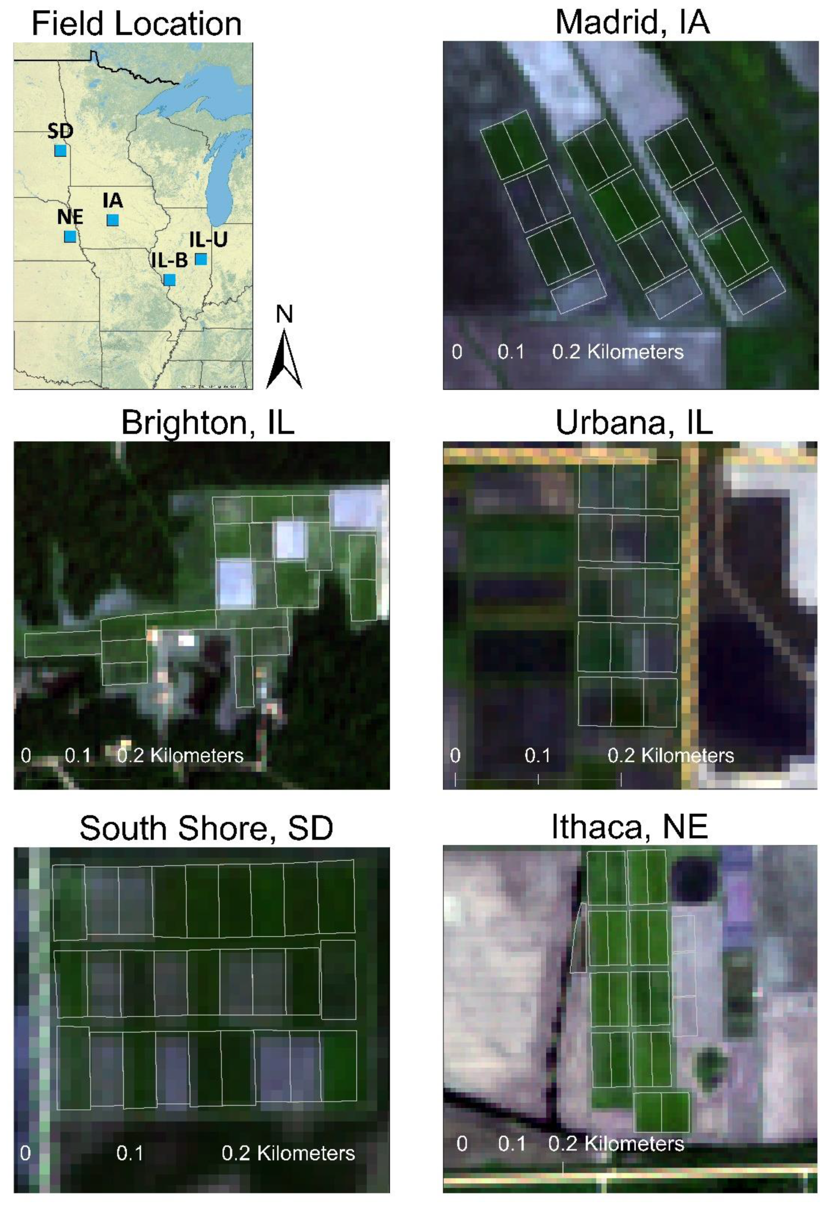
This study comprises five field sites in four U.S. Midwest states, including two sites in Illinois (Brighton (39°3′23.23″ N, 90°11′7.62″ W) and Urbana, Illinois (40°4′7.68″ N, 88°11′26.78″ W)) and one site each in Iowa (Madrid (41°55′52.17″ N, 93°45′49.28″ W)), Nebraska (Ithaca (41°8′57.54″ N, 96°27′14.07″ W)), and South Dakota (South Shore (45°6′20.30″ N, 97°3′42.41″ W)) (Figure 1 and Figure 2). All sites selected for this study are considered marginal based on the landowner’s observation of historical production data. In particular, the production costs of traditional row crops such as corn, soybean, and wheat have been generally higher than the income from yields generated, resulting in an economic loss for the producers. The landowners’ observations also suggest that historical row crop yields for these sites have been 25–50% lower than the county- or state-reported averages. In most cases, the reduced yields are a result of poor soil quality due to soil erosion (i.e., loss of nutrient-rich topsoil) and soil moisture impediments (e.g., too dry, poorly drained, or high nutrient leaching).
Field site characteristics and crop management are included in Table 1. Precipitation data were provided by on-site or locally available weather stations. Treatments (three replicates each) and planting design varied across the site locations based on field (size and arrangement) and climate (temperature) conditions. The switchgrass cultivars and other warm-season perennial grasses evaluated are shown in Figure 1. The switchgrass cultivars included in the study consist of upland (‘Carthage’, ‘Sunburst’, ‘Shawnee’), lowland (‘Independence’), and mixed (hybrid: ‘Liberty’) ecotypes. Switchgrass was planted in the spring of 2019 at three of the five sites (i.e., Brighton, IL; Iowa; and South Dakota). Lowland ecotypes such as ‘Independence’ and ‘W105L’ were also planted at the South Dakota site; however, due to heavy winterkill in 2019, the plots were replanted with soybean and winter wheat for subsequent years and, therefore, are not included in Table 1. The majority of the Nebraska site was planted in 2012, including the Liberty switchgrass, big bluestem mixture (‘Goldmine’ and ‘Bonanza’), and a low diversity mixture (side-oats grama, Indiangrass, big bluestem), and the exception was a single plot of Independence switchgrass, which was planted in the spring of 2019. The Urbana site was the most recently established site, with a spring planting in 2020 (Table 1). All sites were planted with a no-till drill with a targeted planting rate of 300 seedlings/m2 and a 15–18 cm row spacing. Switchgrass stand establishment was evaluated in the fall of the planting year or the following spring using a frequency grid [46]. Plots with an average frequency of less than 25% were overseeded the following season. For the Iowa, South Dakota, and Brighton sites, no large-scale harvest occurred at the end of the establishment year. Instead, biomass was removed (via burning, mowing/raking) in early 2020 prior to the start of new growth. Additional management information and soil data for each site are included in Table S1.

2.2. Data

The data used for modeling were (1) switchgrass yields measured at harvest between November and December 2020 for the five study sites and (2) 10 m resolution Sentinel-2 satellite imagery from the 2020 April–October period. To monitor ground conditions, plot pictures and field observations including chlorophyll content of upper canopy leaves using a SPAD-502 chlorophyll meter (Minolta, Konica Minolta Sensing Europe B.V.) were collected during the growing season. Perennial grass dry yield was collected after a killing frost (air temperature below −2.2 °C) in the fall of 2020 from each study site. At the Iowa, Nebraska, and Brighton sites, full plot biomass was measured by cutting the entire plot with a mower at a cutting height of 10–15 cm. Subsamples of cut biomass were collected from the windrows for measuring moisture and dry matter contents. The windrows were then baled and weighed. In South Dakota, the plots were also mowed and baled, but only a swath (5.5 m in width) up the center of each plot was cut and baled for biomass yield. Subsamples were also collected from the windrows, but the moisture content of the bales was directly measured using a moisture probe. Harvested area was measured for each plot across all field sites. A small-plot combine harvester (Wintersteiger Cibus plot harvester with 4′ Kemper row independent cutter head, Service Point, IA) was used in Urbana to collect biomass yield from three areas in each plot (1.2 m × 9 m). We avoided whole-plot harvest to ensure the stand health during the establishment year. Biomass weight was directly measured by the harvester for each cut section, and subsamples of the cut biomass were collected from the combine for measuring moisture content.
The perennial grass yield dataset available for the model development is summarized in Table 2. The number of data points (or plots) ranged from 12 (Urbana and South Dakota) to 19 (Nebraska). Except for the Nebraska site, the ranges of yields were similar, ranging from 3.16 to 4.66 Mg/ha across the study fields. The low yields at the Urbana site (i.e., 1.16–4.35 Mg/ha) relative to other sites were expected as 2020 was the establishment year for this site (Table 2).
Sentinel-2 satellite bottom-of-atmosphere reflectance images from April to October 2020 were obtained from the Copernicus Open Access Hub (https://scihub.coperni-cus.eu/ (accessed on 24 February 2020)). The time period was selected based on warm-season perennial grass phenology in the Midwest region with green-up period typically occurring in April or May and senescence occurring between September and October. Images with apparent cloud cover over the study sites based on visual interpretation were excluded from the download. Of the 37 images for each site (185 images total), a total of 61 Sentinel-2 multispectral images across the five study sites were obtained (Table 3). The Sentinel-2 multispectral imagery of the five study sites is shown in Figure 3. The optical bands (i.e., blue, green, red, and near-infrared (NIR) bands) at 10 m resolution and the scene classification map at 20 m resolution were used for the model development. The spectral reflectance profiles of each of the five study sites are provided in Figure S1.

2.3. Image Processing and Model Development

The model development consists of image preparation, spectral index calculation, and linear regression model development. Prior to the index calculation, pixels affected by cloud and its shadow in each of the Sentinel-2 bottom-of-atmosphere reflectance images were excluded using the scene classification map layer on the same date, which is a part of Sentinel-2 products identifying several classes including clouds, cloud shadows, and saturated and defective pixels in the image (https://sentinels.copernicus.eu/web/sentinel/technical-guides/sentinel-2-msi (accessed on 7 December 2020)). A total of 20 spectral indices that are known to correlate with vegetation properties were calculated using the images (Table 4). The index values of pixels located only well within the boundaries of each of the plots were extracted to avoid possible spectral contamination from adjacent ground cover. The correlation between each index on each image date with yield was examined, and the index on a single date having the highest correlation with yields was identified.
A linear regression model for estimating yields was developed using the values from one of the index layers having the highest correlation with at-harvest yields. The model was developed using 75% of the available pixels from each plot and validated with the measured plot yields using the remaining 25% of the pixels in order to work with the limited data points. This process was iterated 31 times, and coefficient of determination (R2), mean absolute error (MAE), and root mean squared error (RMSE) were calculated to evaluate the accuracy of yield estimates. For each site, each R2, MAE, and RMSE were averaged over the iterations, and those average values were used as the measure of predictive power of the model for the at-harvest yields for each site. A single linear regression model was developed for each site instead of multiple models for each cultivar due to the limited availability for yield estimates at harvest.

3. Results

3.1. Analysis of Spectral Vegetation Indices in Relation to Switchgrass Yields

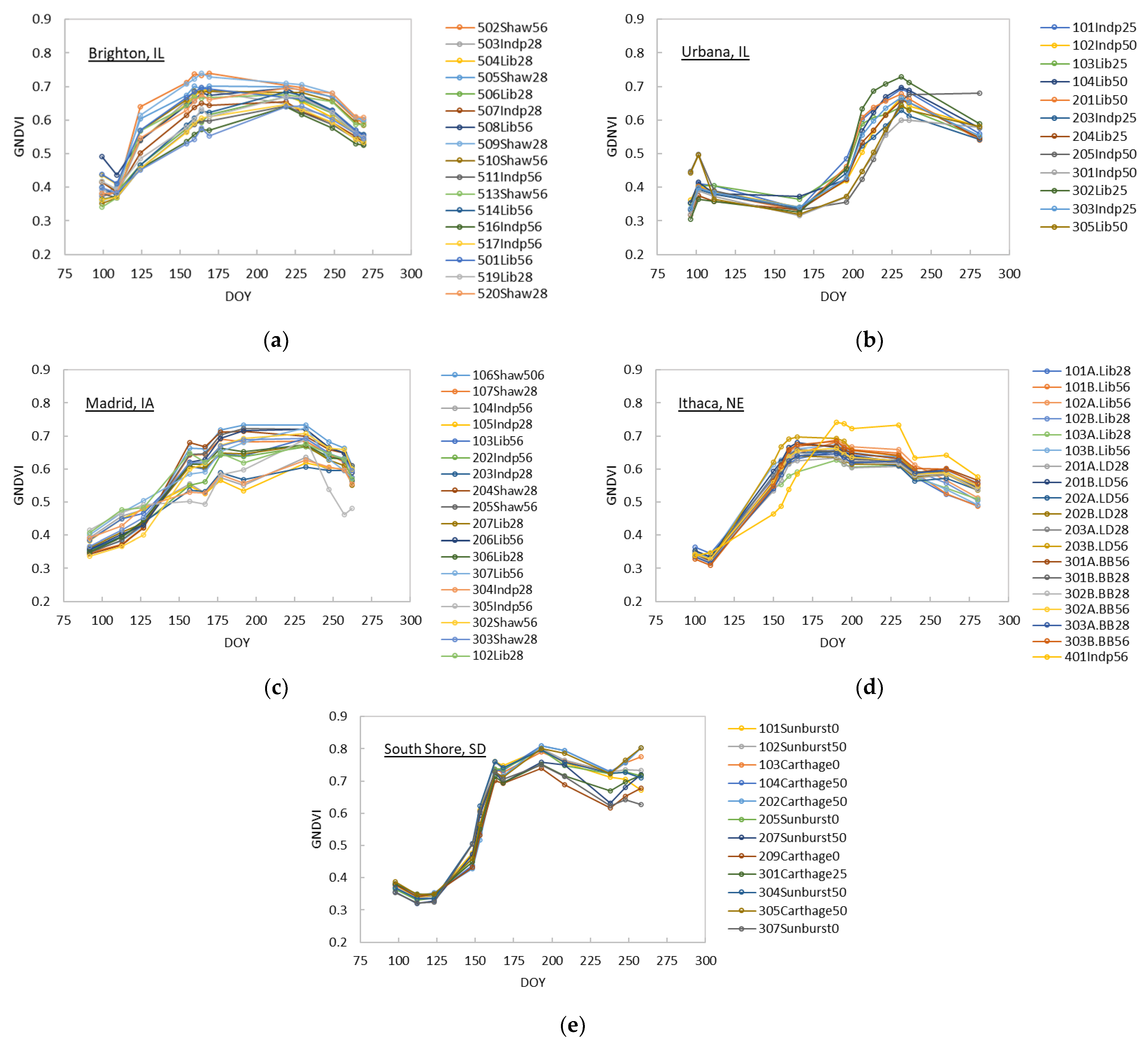
Of the 20 spectral vegetation indices calculated using the 10 m resolution Sentinel-2 multispectral imagery from April to October 2020, the seasonal trajectories of the green normalized difference vegetation index (GNDVI) [58,59] for the five study sites are shown in Figure 4 as examples since the trajectory of GNDVI seemed to represent the trajectories of indices that were highly correlated with harvestable biomass yields, which is described later in this section. The GNDVI values increased from early May and reached the peak greenness around mid-June at the Iowa, Brighton, and Nebraska sites. The South Dakota site, which is the furthest north in latitude, had a later start for greenness increase. The greenness at the Urbana site, the youngest of the five sites, did not start to increase until late June to beginning of July and exhibited a unique greenness trajectory.
In general, the trajectories of index values were very similar across the crops/cultivars within each site, with some exceptions. In particular, the Nebraska site showed very uniform trajectories across the crops (Figure 4: liberty switchgrass, big bluestem, and the low diversity mix). The major exception was the Independence switchgrass plot. The GNDVI trend was outside the 2 standard deviations from the mean. Although the stand of Independence switchgrass (height and thickness) at the Nebraska location looked very different from the other crop plots, due to the lack of plot replication, it is difficult to verify the cause of this variation. With the current dataset, the exclusion of the plot increased the R2 between GNDVI and the harvested yield from 0.313 to 0.873. Therefore, the Independence plot was excluded from the model development for the Nebraska site. The other observed visual crop difference at the Nebraska site occurred after day-of-year (DOY) 260. The GNDVI values for Liberty switchgrass declined more quickly than those for the low diversity mixture and big bluestem plots, resulting in a more defined split between the crop types by the end of the growing season.
In Brighton, a similar split in GNDVI trends between switchgrass cultivars was observed until DOY 219 (Figure 4). Shawnee switchgrass maintained higher GNDVI values than Independence and Liberty switchgrass by the end of the season. At the Iowa site, the majority of the Independence switchgrass plots had lower GNDVI values for the bulk of the growing season (DOY 157–247) compared to the other cultivars, resulting in a greater spread in GNDVI values by cultivar type for this time period. Plot 305, shown in gray in Figure 4, showed a unique trajectory in GNDVI values across the season. In fact, this plot was reseeded at the end of August 2020 due to low plant density (i.e., <25% threshold). In contrast to plot 305, the other two plots in Iowa that required reseeding (i.e., plots 307 (Liberty switchgrass) and 104 (Independence switchgrass)) showed comparable GNDVI trajectories across the season to other plots of the same cultivar type. Although no distinct pattern in GNDVI trajectory specific to any switchgrass cultivar type was observed, the South Dakota and Urbana sites showed variation in late June through the end of the season. Similar overall patterns in seasonal trajectory were observed for other spectral vegetation indices.
Correlations between the spectral vegetation indices and dry biomass yield at harvest are summarized in Table 5. The strength of correlation between the index values and the dry biomass yields at harvest greatly varied across the sites. For the South Dakota site, 17 out of the 20 indices showed R2 > 0.75, while index–yield correlations were moderate to high for the Brighton site (e.g., modified soil-adjusted vegetation index (MSAVI) [63], R2 = 0.661). For the Iowa, Urbana, and Nebraska sites, a few indices showed strong correlations with yields, including the green chlorophyll index (GCI [56], R2 = 0.828, 0.739, 0.884, and 0.878 for the Urbana, Iowa, Nebraska, and South Dakota sites, respectively) and GNDVI (R2 = 0.842, 0.776, 0.873, and 0.857 for the Urbana, Iowa, Nebraska, and South Dakota sites, respectively). The indices based on the soil-adjusted vegetation index (SAVI [68]) were also correlated with the biomass yields for the Iowa site (R2 = 0.737, 0.738, and 0.737 for SAVI, MSAVI, and optimized SAVI (OSAVI) [66], respectively) and Brighton site (R2 = 0.643 across SAVI, MSAVI, and OSAVI). The modified simple ratio index showed a good correlation for the Urbana and Nebraska sites as well (R2 = 0.743 and 0.827, respectively) (Table 5). The average switchgrass plant frequencies across cultivars in Iowa and Brighton (30% and 46%, respectively) in the spring/summer of 2020 were lower than those of the other field sites (Nebraska 85%, Urbana 50%, South Dakota 100%). These two sites also had the largest range in switchgrass plant frequency compared to the other sites.
The strongest correlations of the index values with yields also varied by timing (Table 5). The indices in June (DOY 155–180) showed strong correlation with the dry biomass yields at harvest for the Brighton, Nebraska, and Iowa sites. For the Urbana site, the index–yield correlations were strong in the late growing season (i.e., early October). For the South Dakota site, the correlations varied across the indices.
Of the 20 indices examined, indices utilizing the green and NIR spectral bands such as GCI and GNDVI were consistently identified as those strongly correlated with the yields across the sites (Table 5). The correlations of the indices using the green and NIR spectral bands were stronger than those of indices based on the red and NIR bands (e.g., NDVI) that are commonly used for vegetation studies. Based on the observation of a nearly consistent strong correlation of GNDVI with at-harvest biomass yields across the study sites, the subsequent modeling was carried out exclusively using GNDVI.
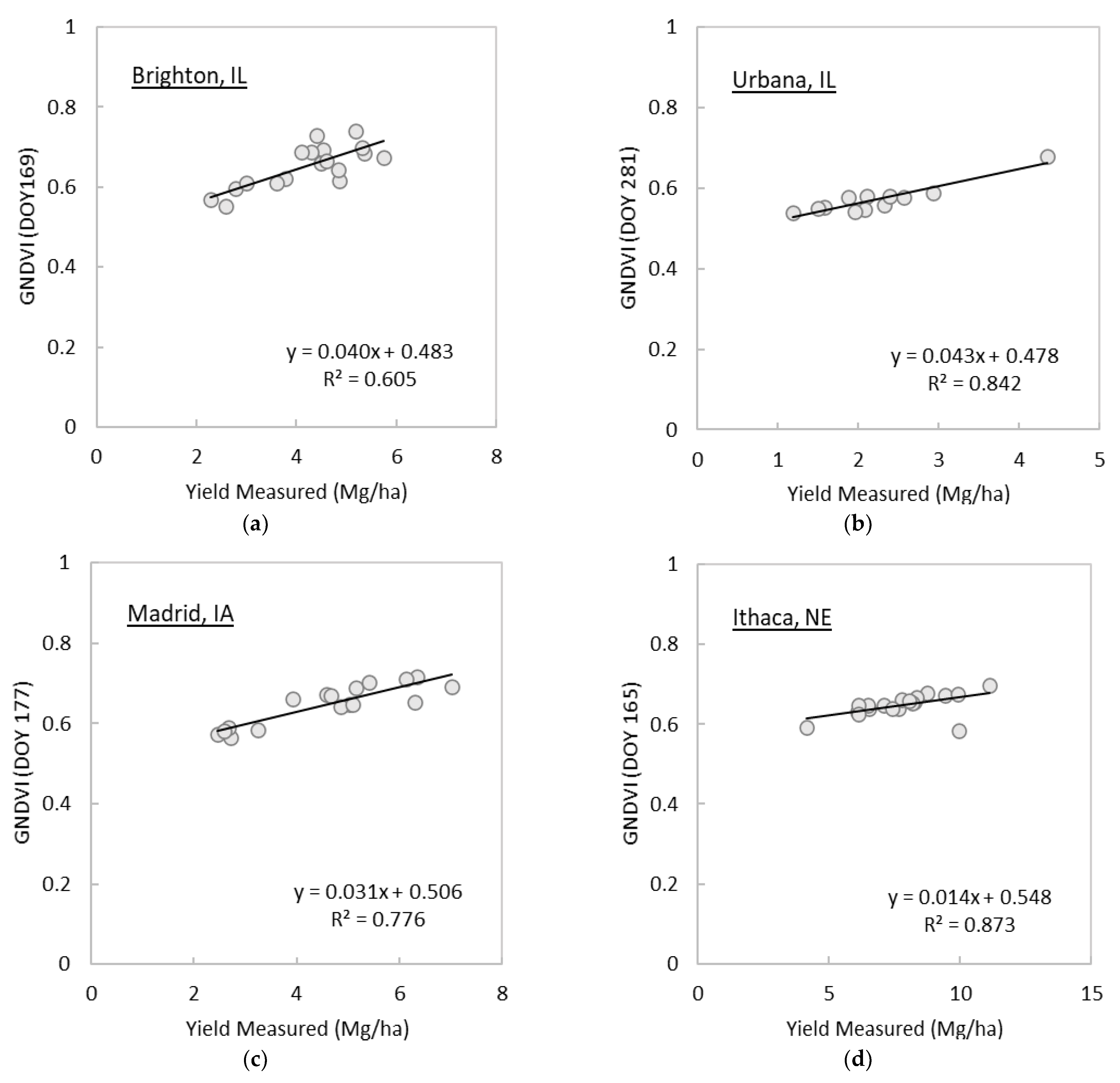
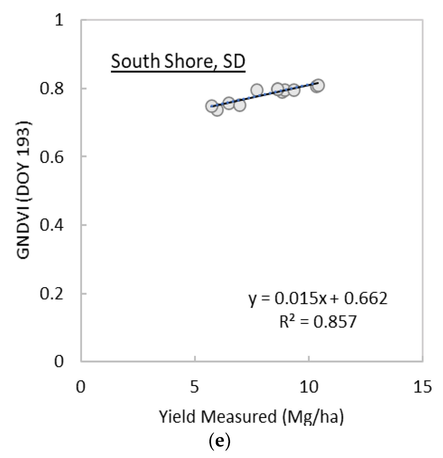
Scatter plots of the harvested dry biomass yields and the average GNDVI values corresponding to each of those plots on the date of highest correlation for each study site are presented in Figure 5. All sites except for the Brighton site showed strong correlations between GNDVI and yield (R2 > 0.75). The GNDVI–yield correlation was moderate for the Brighton site, but index–yield correlations across the indices examined were lower than those of the other sites. Thus, modeling yield using GNDVI was reasonable for this study; GNDVI was calculated using Equation (1):
GNDVI = [NIR − G]/[NIR + G] = [B8 − B3]/[B8 + B3],
where NIR and G are bottom-of-atmosphere reflectance values of the NIR and green spectral bands, which correspond to the spectral band 8 (B8) and band 3 (B3) of Sentinel-2 satellite imagery, respectively.

3.2. Prediction of Switchgrass Dry Biomass Yields at Harvest

The overall performance of the linear regression models using GNDVI for predicting perennial grass dry biomass yields at harvest for the five sites is summarized in Table 6, along with the characteristics of dry biomass yield data used for the model development. Based on the 31 iterations, the yields predicted using the GNDVI linear regression model showed moderate to strong correlations with at-harvest yields ranging from R2 = 0.592 (Brighton) to R2 = 0.879 (South Dakota). The average of MAE ranged from 0.377 Mg/ha (Urbana) to 0.589 Mg/ha (Brighton), and the average of RMSE ranged from 0.399 Mg/ha (Urbana) to 0.685 Mg/ha (Brighton). The average MAE and RMSE indicated that the yields predicted by the GNDVI linear regression model had comparable errors across the five sites, except for the Urbana site, which is characterized by the lowest minimum and maximum measured yields and the smallest measured yield range (Table 2 and Table 6).
The yields predicted by the GNDVI linear regression model showed stronger correlations for the sites having higher minimum and maximum measured yields at harvest (i.e., Nebraska and South Dakota) than for those having lower minimum and maximum yields (i.e., Urbana and Brighton) (Table 2 and Table 6). The predicted yields also correlated more strongly with the measured yields for the sites having the greater range of measured yields (i.e., Nebraska and South Dakota) than those with the limited yield range (i.e., Urbana and Brighton).
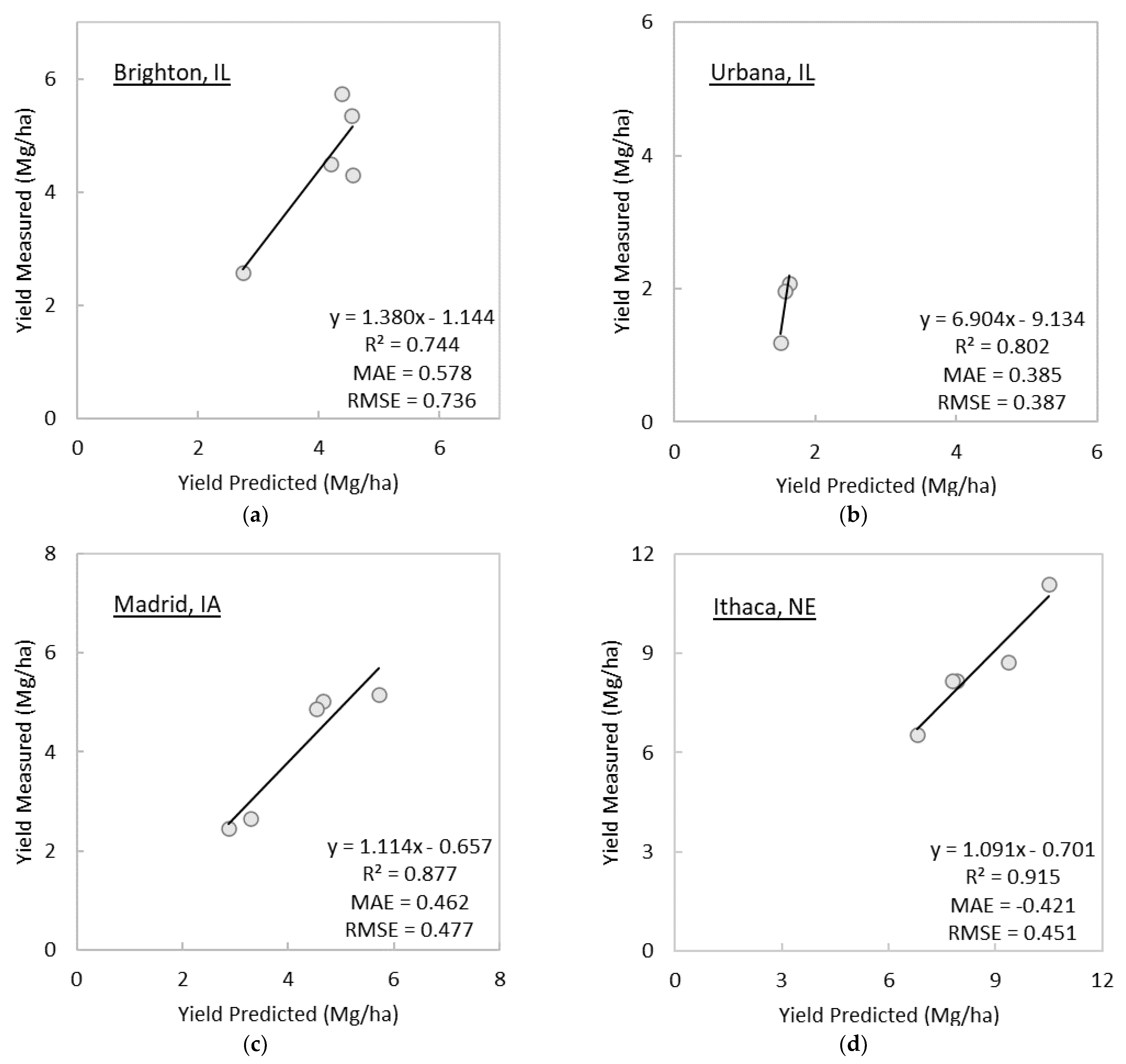
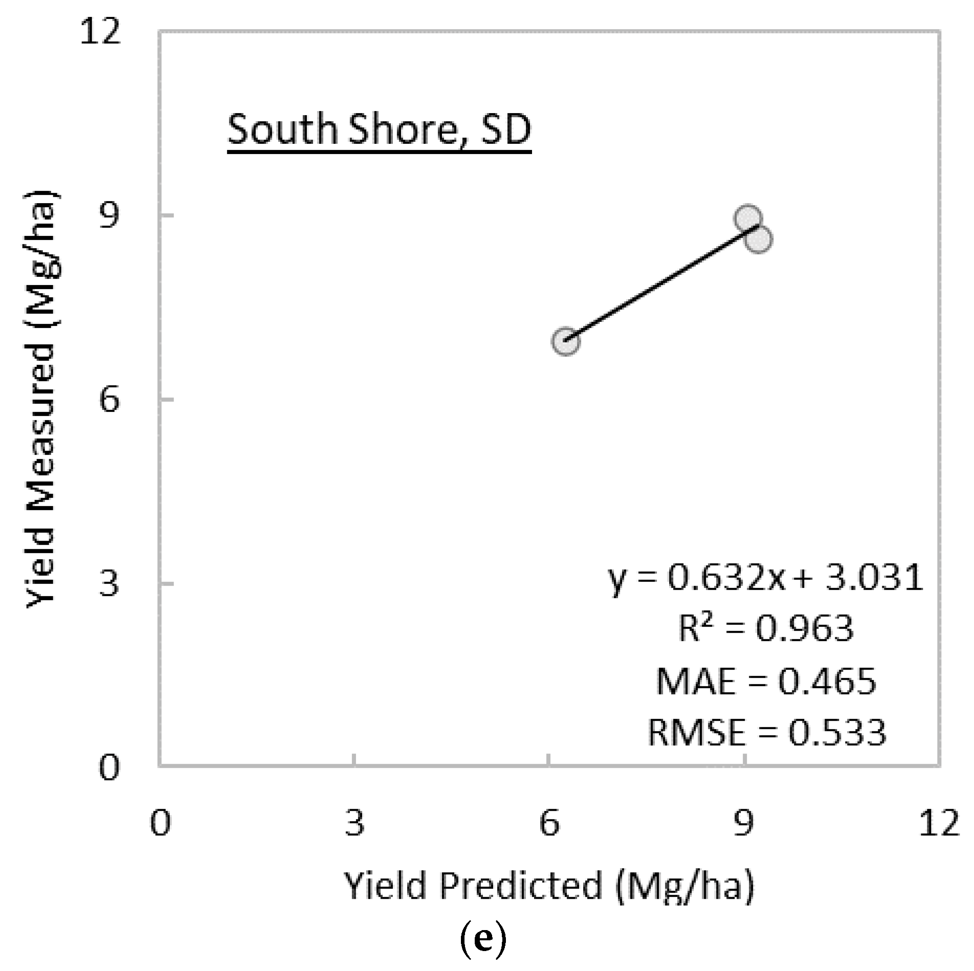
Examples of scatter plots of the measured switchgrass yields at harvest and predicted yields are presented in Figure 6. Each scatter plot was selected from the iteration resulting in the median R2 for each site. Specific performance measures would vary across iterations, but the predicted yields showed a strong linear relationship with the measured yields across the five sites. The model showed the lowest median R2 for the Brighton site with a greater difference between RMSE and MAE (Figure 6), which is also suggested in Table 6. The model appears less robust for the Urbana site than other sites, as indicated by the slope and intercept deviating from 1 and 0, respectively, in the example (slope = 6.904, intercept = 9.134, Figure 6).
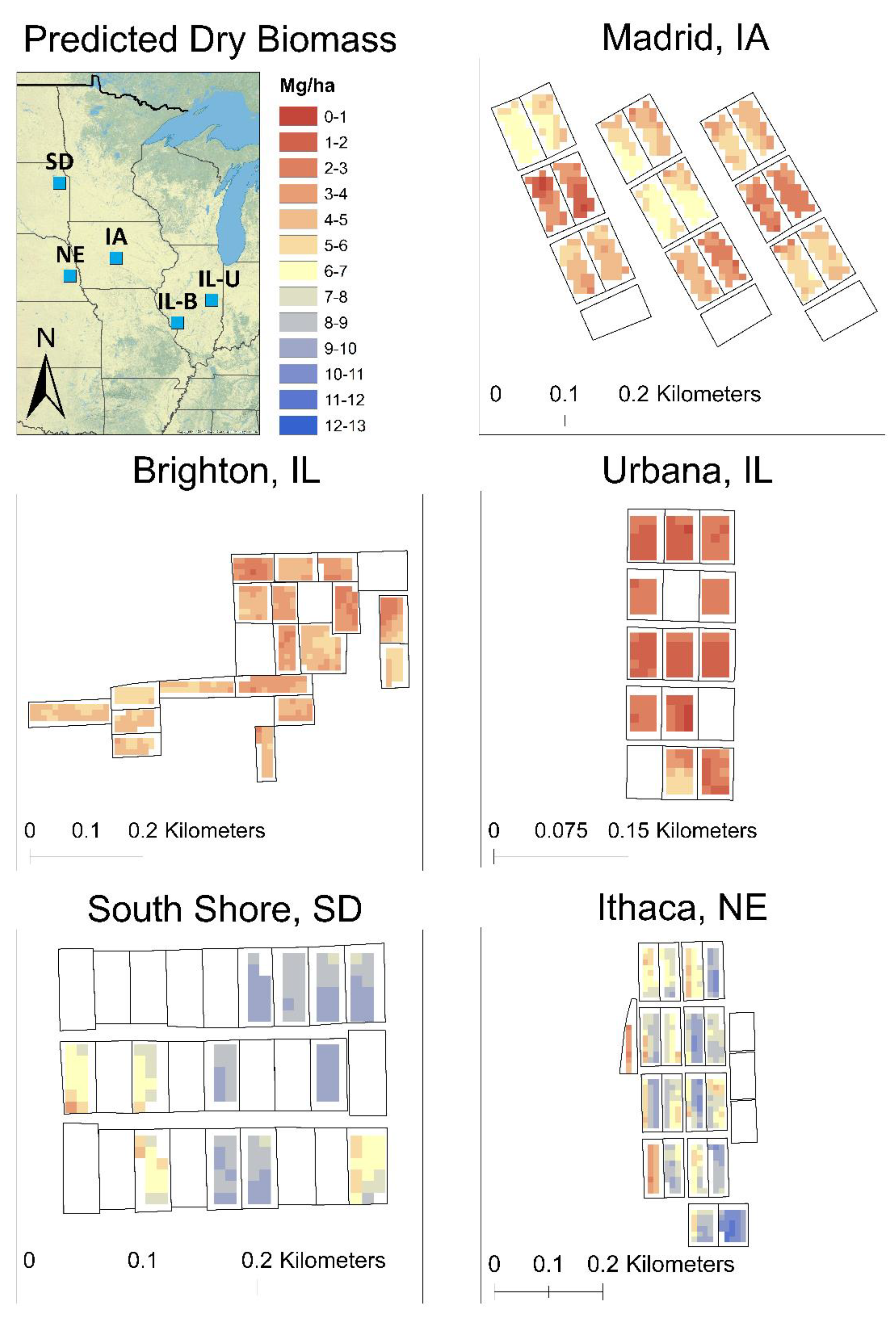
Examples of the switchgrass dry biomass yields for the five study sites that were predicted using the GNDVI linear regression model are shown in Figure 7. The maps were generated by applying the model developed using plot-level data to image pixels. Overall, the relative yield (i.e., high and low yields) and variation of predicted yields reflect the amount and range of the measured yields across the sites (Table 2). For example, the Urbana site, which has the lowest minimum and maximum measured yields (i.e., 1.19–4.35 Mg/ha) and the smallest yield range (i.e., 3.16 Mg/ha) of all sites, showed the lowest predicted yields and the most limited variation across the site. In contrast, the Nebraska site, which has the largest measured yield range (i.e., 6.96 Mg/ha) of all sites, exhibited the greatest variation in the predicted yields (Table 2 and Figure 7). Across crop types at the Nebraska site, the highest yields occurred in plots fertilized with 56 kg N ha−1 compared to 28 kg N ha−1. Relationships between the predicted yields and fertilizer application were also observed for some plots in other sites (Figure 1 and Figure 7). For the South Dakota site, the model predicted relatively homogeneous yields within each of the high-yielding plots but predicted noticeable internal variation for the plots having moderate to low yields. The difference between higher- and lower-yielding plots was not always associated with fertilizer rate (Figure 1 and Figure 7). For the Brighton and Iowa sites, switchgrass cultivar type can be seen contributing to yield variation (Figure 1 and Figure 7).

4. Discussion

Despite the limited data available, the simple linear regression model using GNDVI showed promise for predicting harvestable switchgrass dry biomass yields at a plot scale (i.e., 0.2–0.4 ha). Except for the Urbana site, calculated index values in midsummer (i.e., DOY 165 through 193) were often strongly correlated with the perennial grass yields at harvest for all sites across the spectral vegetation indices examined (R2 as high as 0.879; MAE and RMSE as low as 0.539 Mg/ha and 0.616 Mg/ha, respectively, except for the establishment year). Switchgrass and other warm-season perennial grasses often accelerate their growth in June followed by flowering, which was observed to start by the middle to end of July for most cultivars. Because plants shift their energy allocation from vegetative growth to flowering at that time, the greatest correlation between vegetation index values is around the same time, which indicates the maximum green biomass of the season, and at-harvest biomass yield is understandable. This suggests that yields may be fairly reliably predicted a few months before harvest. In this study, the harvestable dry biomass yields were predicted 152 days prior to harvest on average. Factors that could influence the prediction accuracy when using midsummer spectral index values include the amount of precipitation, such as prolonged droughts that would influence soil moisture status. Sources of uncertainty in predicted yields could also include timing of harvest as observed in our previous study (not published) and cultivar variation in physiology and chemistry as they determine plant spectral responses [72]. Because fertilizer and herbicide applications and tillage practices influence the nitrogen status of crops [42,43,44], the amount of exposed ground within the stands [45], and the composition of exposed ground (e.g., crop residues and weeds) [44,45], these factors should also be carefully considered when modeling yields using spectral vegetation indices.
Another source of uncertainty in predicting switchgrass yields is associated with image availability. The availability of Sentinel-2 imagery for switchgrass yield prediction is constrained by periods of high cloud cover, which is a common limitation for satellite imagery. In this study, a total of 185 images were available for the study sites from April to October 2020. However, only 61 images were obtained and utilized in subsequent analyses across the sites (Table 3). For many of the sites, satellite imagery around the time of flowering (mid to end of July for most grasses and switchgrass cultivars, except for Independence switchgrass which flowers closer to the end of August) was not available due to cloud cover. This raised a question on the likelihood of satellite image availability that could provide sufficient predictive power for at-harvest biomass yields for each site. Even though the GNDVI seasonal trajectories show fairly comparable values around the selected image dates across the sites, the impact of image dates on yield prediction is uncertain. Furthermore, due to cloud cover, the availability of imagery during the summer months in subsequent years for multiyear studies is also not guaranteed. Although unmanned aerial vehicles and other technologies have been utilized to mitigate the issue of cloud cover, these technologies can be time-consuming and costly and could require rigorous data processing for proper analysis. Technologies that could increase satellite image availability or methodologies for simulating seasonal trajectory would greatly help in reducing such uncertainty.
The comparison of 20 spectral vegetation indices showed that the NIR spectral band is the key to predicting biomass yields, which is consistent with a number of existing vegetation studies using remote sensing [15,73]. The index comparison also indicated a greater information value of the green spectral band for predicting at-harvest yields of switchgrass and other warm-season perennial grasses than the red band. Gitelson et al. [58,59] found that spectral reflectance in the green spectral region is more sensitive to plant chlorophyll content than that in the red spectral region. As a result, GNDVI showed a stronger correlation with chlorophyll contents across the plants examined than NDVI, which utilizes the NIR and red bands [59]. Switchgrass aboveground biomass is accumulated through vegetative growth or elongation of stems from emergence in the spring through flowering, with the growth period (green-up to anthesis) dependent upon geographic location (temperature and daylength) and ecotype [74,75,76]. During the vegetative growth period, plant chlorophyll content increases [75]. This pattern was observed in the Iowa, Brighton, and Nebraska sites with green-up observed in imagery to occur in late April/early May and continue into June and July, which corresponded to the measured chlorophyll content in the field during this time. In mid- to late summer, the GNDVI values plateaued, which appeared to coincide with flowering. Then, GNDVI values gradually decreased as switchgrass began senescing.
The pattern observed between the predictive power of the GNDVI linear regression model measured by R2 and the characteristics of measured yields (i.e., minimum, maximum, and range) may be explained by the strength of spectral signal associated with switchgrass/perennial grass biomass in the field during the image collection. Dense switchgrass growth, which would indicate greater biomass volume than sparse growth, is likely represented by pixel values in the image. In contrast, spectral signals from sparse switchgrass growth likely contain noise from background such as soil or plant residue and obscure true signals of switchgrass in pixel values. Although it is out of scope for the present study, the influence of vertically projected cover and height of switchgrass and presence of other materials on remote sensing-based yield prediction could be examined with field observations of plant height, canopy photos, and weed cover during the peak growing season.
Phenological variations observed in the GNDVI seasonal trajectories can reflect the age of switchgrass or perennial grass stands and geographic location. The later start of the greening at the South Dakota site compared to the other sites can be explained by its higher latitude and colder temperatures later in the spring compared to the other sites. The unique greenness pattern of cultivars for the Urbana site can be explained by the stand age. Because the study year (2020) was the establishment year for this site, the timing of biomass accumulation was expected to be different from the other sites. The delayed increase in GNDVI can in part be due to the planting date (DOY 141) and the slow establishment, which is typical of perennial crops. Additionally, literature has shown that switchgrass flowering during the establishment year can occur later than what is observed in the following years after establishment [77].
At the Nebraska site, the difference in GNDVI seasonal trajectory between Independence switchgrass and the other perennial grasses may also be associated with differences in stand age. The Independence plot was established in 2019 while the other plots were established in 2012. The differences may also be associated with phenological characteristics such as canopy structure and leaf chlorophyll. The Independence stand was taller and thicker than the other perennial grasses and Liberty switchgrass cultivar in 2020. It also has a bluer leaf coloration with a waxy coating compared to the other switchgrass cultivars and perennial grasses used in this study. However, due to the lack of plot replication at the Nebraska site along with other phenological data, it is difficult to determine the causes of variation at this time. Additional years of data, collection of phenological data across cultivars, and observing trends between cultivar types across the other field locations may shed light on these seasonal trends. The GNDVI trajectory showed patterns specific to cultivar types at some sites, which suggests that cultivar-specific yields may be modeled using optical imagery with a sufficient number of replicate plots for each cultivar type. This could help the selection of high-yield cultivars.

5. Conclusions

This paper presented the initial investigation on the predictive power of spectral vegetation indices derived from optical satellite imagery, more specifically GNDVI, for at-harvest switchgrass and other warm-season perennial dry biomass yields using a linear regression model. The study utilized 10 m resolution Sentinel-2 multispectral imagery that was collected from April to October 2020 over the five study sites located in the U.S. Midwest states—Iowa, Illinois, Nebraska, and South Dakota. The key findings of the study were as follows:
  • The linear regression model using midsummer GNDVI predicted at-harvest perennial grass yield with R2 as high as 0.879 and MAE and RMSE as low as 0.539 Mg/ha and 0.616 Mg/ha, respectively, except for the establishment year. The selection of image date in this study was based on image availability; thus, there is a possibility that the GNDVI linear regression models has a greater predictive power for at-harvest yields than presented in this study.
  • The GNDVI linear regression model predicted at-harvest switchgrass yields as early as 152 days before the date of harvest on average, except for the year of establishment. More frequent cloud-free imagery than used in the present study or simulated seasonal trajectories of spectral vegetation indices could allow us to answer more precisely how early and accurately at-harvest yields can be predicted using remote sensing.
  • While the NIR spectral band was found to be one of the key spectral bands, the green band appeared to have a greater contribution for predicting at-harvest switchgrass and other perennial grass dry biomass yields than the red band. This is consistent with existing studies [58,59] demonstrating that the sensitivity of the green spectral reflectance to plant chlorophyll content, which is indicative of green biomass volume, is greater than that of the red spectral reflectance.
The model formulated in this study will be further tested using additional datasets from 2021. Downscaling of the model should also be explored to estimate switchgrass and other warm-season perennial grass yields at a 10 m scale, which would enable the integration of the data into a predictive model for marginal lands. Additional future studies will include determining (1) if a single-date spectral vegetation index from the optimal available image would provide satisfactory at-harvest switchgrass yield prediction, (2) if simulated seasonal trajectories of a spectral vegetation index could improve accuracy and robustness of switchgrass yield prediction, (3) how early switchgrass yields can be predicted using remote sensing, (4) if remote sensing models developed for a limited number of sites using one year could be applicable for predicting switchgrass yields of other years and other sites, and (5) how vertically projected cover and height of switchgrass and presence of other materials would influence remote sensing-based yield prediction. Additional areas of research include the uniqueness of establishment year for estimating harvestable switchgrass yields and potential impacts of herbicide and fertilizer treatments and tillage practices on biomass yield estimate using remote sensing.
In addition to biomass yields, an ability to predict biomass moisture and nutrient content at harvest in advance would provide actionable information to biorefineries in planning storage, transport, and adjustment to conversion formulas or preprocessing. Thus, predictive modeling for biomass moisture and nutrient content using remote sensing should also be explored.

Supplementary Materials

The following are available online at https://www.mdpi.com/article/10.3390/land10111221/s1, Figure S1: The spectral reflectance profile of the five study sites; Table S1: Additional field characteristics and management data, Table S2: Plant frequency across perennial grass crops/cultivars in the spring–summer of 2020.

Author Contributions

Conceptualization, Y.H., C.R.Z. and J.F.C.; methodology, Y.H., D.L., C.R.Z., C.-H.L., E.H., A.B. and R.M.; validation, Y.H.; formal analysis, Y.H. and C.R.Z.; data curation, C.R.Z., D.L., C.-H.L., E.H., A.B. and R.M., writing—original draft preparation, Y.H., C.R.Z. and J.F.C.; writing—review and editing, D.L., C.-H.L., E.H., A.B., R.M. and M.C.N.; visualization, C.R.Z. and Y.H.; project administration, J.F.C.; funding acquisition, D.L., J.F.C. and M.C.N. All authors have read and agreed to the published version of the manuscript.

Funding

This research was funded by the U.S. Department of Energy, Energy Efficiency and Renewable Energy, Bioenergy Technologies Office, grant number DE-EE0008521. This research was supported by the USDA Agricultural Research Service (USDA-ARS). USDA is an equal opportunity provider and employer. This manuscript has been created by UChicago Argonne, LLC, Operator of Argonne National Laboratory (“Argonne”). Argonne, a U.S. Department of Energy (DOE) Office of Science laboratory, is operated under Contract No. DE-AC02-06CH11357. The U.S. Government retains for itself, and others acting on its behalf, a paid-up nonexclusive, irrevocable worldwide license in said article to reproduce, prepare derivative works, distribute copies to the public, and perform publicly and display publicly, by or on behalf of the Government.

Institutional Review Board Statement

Not applicable.

Informed Consent Statement

Not applicable.

Data Availability Statement

The data presented in this study are available on request from the corresponding author.

Acknowledgments

The authors would like to thank Nicholas Boersma at Iowa State University, Steve Masterson at USDA-ARS, all the students, and staff members from all partner organizations who have assisted in data collection, site management, and coordination. Without them, this work would not have been possible. The authors also thank all anonymous reviewers for insightful comments and constructive criticism to improve the quality of this manuscript.

Conflicts of Interest

The authors declare no conflict of interest.

References

  1. Dietz, T.; Börner, J.; Förster, J.J.; Von Braun, J. Governance of the bioeconomy: A global comparative study of national bioeconomy strategies. Sustainability 2018, 10, 3190. [Google Scholar] [CrossRef] [Green Version]
  2. Duncan, M. US Federal initiatives to support biomass research and development. J. Ind. Ecol. 2003, 7, 193–201. [Google Scholar] [CrossRef]
  3. Board, B. The Bioeconomy Initiative: Implementation Framework. 2018. Available online: https://biomassboard.gov/sites/default/files/pdfs/Bioeconomy_Initiative_Implementation_Framework_FINAL.pdf (accessed on 4 December 2020).
  4. Golden, J.S.; Handfield, R.B.; Daystar, J.; McConnell, T.E. An economic impact analysis of the US biobased products industry: A report to the Congress of the United States of America. Ind. Biotechnol. 2015, 11, 201–209. [Google Scholar] [CrossRef]
  5. Langholtz, M.H.; Stokes, B.J.; Eaton, L.M. 2016 Billion-ton report: Advancing domestic resources for a thriving bioeconomy, Volume 1: Economic availability of feedstock. In Oak Ridge National Laboratory, Oak Ridge, Tennessee, Managed by UT-Battelle, LLC for the US Department of Energy (DOE); U.S. DOE Energy Efficiency and Renewable Energy Bioenergies Technologies Office: Washington, DC, USA, 2016; Volume 2016, pp. 1–411. [Google Scholar]
  6. Board, B. Increasing Feedstock Production for Biofuels: Economic Drivers, Environmental Implications, and the Role of Research. 2010. Available online: https://afdc.energy.gov/files/pdfs/increasing_feedstock_revised.pdf (accessed on 1 June 2021).
  7. Mitchell, R.; Schmer, M.; Anderson, W.; Jin, V.; Balkcom, K.; Kiniry, J.; Coffin, A.; White, P. Dedicated energy crops and crop residues for bioenergy feedstocks in the central and eastern USA. Bioenergy Res. 2016, 9, 384–398. [Google Scholar] [CrossRef] [Green Version]
  8. Berndes, G.; Bird, N.; Cowie, A. Bioenergy, Land Use Change and Climate Change Mitigation; IEA Bioenergy Report; ExCo:2010:03. Available online: https://www.osti.gov/etdeweb/servlets/purl/22110326 (accessed on 1 June 2021).
  9. Ssegane, H.; Negri, M.C.; Quinn, J.; Urgun-Demirtas, M. Multifunctional landscapes: Site characterization and field-scale design to incorporate biomass production into an agricultural system. Biomass Bioenergy 2015, 80, 179–190. [Google Scholar] [CrossRef] [Green Version]
  10. Cacho, J.F.; Youssef, M.A.; Chescheir, G.M.; Skaggs, R.W.; Appelboom, T.W.; Leggett, Z.H.; Sucre, E.B.; Nettles, J.E.; Arellano, C. Effects of forest-based bioenergy feedstock production on shallow groundwater quality of a drained forest soil. Sci. Total Environ. 2018, 631, 13–22. [Google Scholar] [CrossRef]
  11. Cacho, J.; Negri, M.; Zumpf, C.; Campbell, P. Introducing perennial biomass crops into agricultural landscapes to address water quality challenges and provide other environmental services. Wiley Interdiscip. Rev. Energy Environ. 2018, 7, e275. [Google Scholar] [CrossRef]
  12. Englund, O.; Dimitriou, I.; Dale, V.H.; Kline, K.L.; Mola-Yudego, B.; Murphy, F.; English, B.; McGrath, J.; Busch, G.; Negri, M.C. Multifunctional perennial production systems for bioenergy: Performance and progress. Wiley Interdiscip. Rev. Energy Environ. 2020, 9, e375. [Google Scholar] [CrossRef]
  13. Ssegane, H.; Negri, M.C. An integrated landscape designed for commodity and bioenergy crops for a tile-drained agricultural watershed. J. Environ. Qual. 2016, 45, 1588–1596. [Google Scholar] [CrossRef]
  14. Schmer, M.R.; Mitchell, R.; Vogel, K.; Schacht, W.H.; Marx, D.B. Spatial and temporal effects on switchgrass stands and yield in the Great Plains. BioEnergy Res. 2010, 3, 159–171. [Google Scholar] [CrossRef] [Green Version]
  15. Ahamed, T.; Tian, L.; Zhang, Y.; Ting, K. A review of remote sensing methods for biomass feedstock production. Biomass and Bioenergy 2011, 35, 2455–2469. [Google Scholar] [CrossRef]
  16. Basso, B.; Cammarano, D.; Carfagna, E. Review of crop yield forecasting methods and early warning systems. In Proceedings of the First Meeting of the Scientific Advisory Committee of the Global Strategy to Improve Agricultural and Rural Statistics, FAO Headquarters, Rome, Italy, 18–19 June 2013. [Google Scholar]
  17. Campbell, J.B. Introduction to Remote Sensing; CRC Press: Boca Raton, FL, USA, 2002. [Google Scholar]
  18. Slaton, M.R.; Raymond Hunt, E., Jr.; Smith, W.K. Estimating near-infrared leaf reflectance from leaf structural characteristics. Am. J. Bot. 2001, 88, 278–284. [Google Scholar] [CrossRef] [PubMed]
  19. Shanahan, J.F.; Schepers, J.S.; Francis, D.D.; Varvel, G.E.; Wilhelm, W.W.; Tringe, J.M.; Schlemmer, M.R.; Major, D.J. Use of remote-sensing imagery to estimate corn grain yield. Agron. J. 2001, 93, 583–589. [Google Scholar] [CrossRef] [Green Version]
  20. Hamada, Y.; Ssegane, H.; Negri, M.C. Mapping intra-field yield variation using high resolution satellite imagery to integrate bioenergy and environmental stewardship in an agricultural watershed. Remote Sens. 2015, 7, 9753–9768. [Google Scholar] [CrossRef] [Green Version]
  21. Johnson, D.M. An assessment of pre-and within-season remotely sensed variables for forecasting corn and soybean yields in the United States. Remote Sens. Environ. 2014, 141, 116–128. [Google Scholar] [CrossRef]
  22. Gao, F.; Anderson, M.; Daughtry, C.; Johnson, D. Assessing the variability of corn and soybean yields in central Iowa using high spatiotemporal resolution multi-satellite imagery. Remote Sens. 2018, 10, 1489. [Google Scholar] [CrossRef] [Green Version]
  23. Cicek, H.; Sunohara, M.; Wilkes, G.; McNairn, H.; Pick, F.; Topp, E.; Lapen, D. Using vegetation indices from satellite remote sensing to assess corn and soybean response to controlled tile drainage. Agric. Water Manag. 2010, 98, 261–270. [Google Scholar] [CrossRef]
  24. Smith, R.; Adams, J.; Stephens, D.; Hick, P. Forecasting wheat yield in a Mediterranean-type environment from the NOAA satellite. Aust. J. Agric. Res. 1995, 46, 113–125. [Google Scholar] [CrossRef]
  25. Dempewolf, J.; Adusei, B.; Becker-Reshef, I.; Hansen, M.; Potapov, P.; Khan, A.; Barker, B. Wheat yield forecasting for Punjab Province from vegetation index time series and historic crop statistics. Remote Sens. 2014, 6, 9653–9675. [Google Scholar] [CrossRef] [Green Version]
  26. Salazar, L.; Kogan, F.; Roytman, L. Use of remote sensing data for estimation of winter wheat yield in the United States. Int. J. Remote Sens. 2007, 28, 3795–3811. [Google Scholar] [CrossRef]
  27. Zhou, X.; Zhu, X.; Dong, Z.; Guo, W. Estimation of biomass in wheat using random forest regression algorithm and remote sensing data. Crop J. 2016, 4, 212–219. [Google Scholar]
  28. Mosleh, M.K.; Hassan, Q.K.; Chowdhury, E.H. Development of a remote sensing-based rice yield forecasting model. Span. J. Agric. Res. 2016, 14, e0907. [Google Scholar] [CrossRef] [Green Version]
  29. Noureldin, N.; Aboelghar, M.; Saudy, H.; Ali, A. Rice yield forecasting models using satellite imagery in Egypt. Egypt. J. Remote Sens. Space Sci. 2013, 16, 125–131. [Google Scholar] [CrossRef] [Green Version]
  30. Tennakoon, S.; Murty, V.; Eiumnoh, A. Estimation of cropped area and grain yield of rice using remote sensing data. Int. J. Remote Sens. 1992, 13, 427–439. [Google Scholar] [CrossRef]
  31. Cicore, P.; Serrano, J.; Shahidian, S.; Sousa, A.; Costa, J.L.; da Silva, J.R.M. Assessment of the spatial variability in tall wheatgrass forage using LANDSAT 8 satellite imagery to delineate potential management zones. Environ. Monit. Assess. 2016, 188, 513. [Google Scholar] [CrossRef] [PubMed]
  32. Serrano, J.; Shahidian, S.; Marques da Silva, J. Monitoring seasonal pasture quality degradation in the Mediterranean montado ecosystem: Proximal versus remote sensing. Water 2018, 10, 1422. [Google Scholar] [CrossRef] [Green Version]
  33. Serrano, J.; Shahidian, S.; Marques da Silva, J. Evaluation of normalized difference water index as a tool for monitoring pasture seasonal and inter-annual variability in a Mediterranean agro-silvo-pastoral system. Water 2019, 11, 62. [Google Scholar] [CrossRef] [Green Version]
  34. Massey, J.; Antonangelo, J.; Zhang, H. Nitrogen Fertilization and Harvest Timing Affect Switchgrass Quality. Resources 2020, 9, 61. [Google Scholar] [CrossRef]
  35. Guretzky, J.A.; Biermacher, J.T.; Cook, B.J.; Kering, M.K.; Mosali, J. Switchgrass for forage and bioenergy: Harvest and nitrogen rate effects on biomass yields and nutrient composition. Plant Soil 2011, 339, 69–81. [Google Scholar] [CrossRef] [Green Version]
  36. Hedtcke, J.L.; Sanford, G.R.; Hadley, K.E.; Thelen, K.D. Maximizing land use during switchgrass establishment in the north central United States. Agron. J. 2014, 106, 596–604. [Google Scholar] [CrossRef]
  37. Sarath, G.; Baird, L.M.; Mitchell, R.B. Senescence, dormancy and tillering in perennial C4 grasses. Plant Sci. 2014, 217, 140–151. [Google Scholar] [CrossRef] [Green Version]
  38. Serapiglia, M.J.; Boateng, A.A.; Lee, D.K.; Casler, M.D. Switchgrass harvest time management can impact biomass yield and nutrient content. Crop Sci. 2016, 56, 1970–1980. [Google Scholar] [CrossRef]
  39. Wilson, D.M.; Heaton, E.A.; Liebman, M.; Moore, K.J. Intraseasonal changes in switchgrass nitrogen distribution compared with corn. Agron. J. 2013, 105, 285–294. [Google Scholar] [CrossRef]
  40. Wang, Z.; Smyth, T.J.; Crozier, C.R.; Gehl, R.J.; Heitman, A.J. Yield and nitrogen removal of bioenergy grasses as influenced by nitrogen rate and harvest management in the coastal plain region of North Carolina. BioEnergy Res. 2018, 11, 44–53. [Google Scholar] [CrossRef]
  41. Zumpf, C.; Lee, M.S.; Thapa, S.; Guo, J.; Mitchell, R.; Volenec, J.J.; Lee, D. Impact of warm-season grass management on feedstock production on marginal farmland in Central Illinois. GCB Bioenergy 2019, 11, 1202–1214. [Google Scholar] [CrossRef] [Green Version]
  42. Sibanda, M.; Mutanga, O.; Dube, T.; Mafongoya, P.L. Spectrometric proximally sensed data for estimating chlorophyll content of grasslands treated with complex fertilizer combinations. J. Appl. Remote Sens. 2020, 14, 024517. [Google Scholar] [CrossRef]
  43. Orsini, R.; Fiorentini, M.; Zenobi, S. Testing vegetation index categories as influenced by soil management and nitrogen fertilization in cereal based cropping systems. In Proceedings of the 2019 IEEE International Workshop on Metrology for Agriculture and Forestry (MetroAgriFor), Portici, Italy, 24–26 October 2019; pp. 13–18. [Google Scholar]
  44. Orsini, R.; Fiorentini, M.; Zenobi, S. Evaluation of Soil Management Effect on Crop Productivity and Vegetation Indices Accuracy in Mediterranean Cereal-Based Cropping Systems. Sensors 2020, 20, 3383. [Google Scholar] [CrossRef]
  45. Schut, A.G.; Traore, P.C.S.; Blaes, X.; Rolf, A. Assessing yield and fertilizer response in heterogeneous smallholder fields with UAVs and satellites. Field Crops Res. 2018, 221, 98–107. [Google Scholar] [CrossRef]
  46. Vogel, K.P.; Masters, R.A. Frequency grid--a simple tool for measuring grassland establishment. Rangel. Ecol. Manag. J. Range Manag. Arch. 2001, 54, 653–655. [Google Scholar] [CrossRef]
  47. Illinois Climate Network: Water and Atmospheric Resources Monitoring Program. Illinois State Water Survey, 2204 Griffith Drive, Champaign, IL 61820-7495. Available online: https://doi.org/10.13012/J8MW2F2Q (accessed on 30 June 2021).
  48. Automated Weather Data Network: High Plains Regional Climate Center. Available online: https://hprcc.unl.edu/awdn/ (accessed on 1 July 2021).
  49. Iowa Environmental Mesonet: Iowa State University. Available online: https://mesonet.agron.iastate.edu/agclimate/hist/daily.php (accessed on 15 June 2021).
  50. South Dakota Mesonet. Available online: https://climate.sdstate.edu/ (accessed on 15 June 2021).
  51. Kaufman, Y.J.; Tanre, D. Atmospherically resistant vegetation index (ARVI) for EOS-MODIS. IEEE Trans. Geosci. Remote Sens. 1992, 30, 261–270. [Google Scholar] [CrossRef]
  52. Tucker, C.J. Red and photographic infrared linear combinations for monitoring vegetation. Remote Sens. Environ. 1979, 8, 127–150. [Google Scholar] [CrossRef] [Green Version]
  53. Huete, A.; Didan, K.; Miura, T.; Rodriguez, E.P.; Gao, X.; Ferreira, L.G. Overview of the radiometric and biophysical performance of the MODIS vegetation indices. Remote Sens. Environ. 2002, 83, 195–213. [Google Scholar] [CrossRef]
  54. Jiang, Z.; Huete, A.R.; Didan, K.; Miura, T. Development of a two-band enhanced vegetation index without a blue band. Remote Sens. Environ. 2008, 112, 3833–3845. [Google Scholar] [CrossRef]
  55. Gitelson, A.A.; Kaufman, Y.J.; Merzlyak, M.N. Use of a green channel in remote sensing of global vegetation from EOS-MODIS. Remote Sens. Environ. 1996, 58, 289–298. [Google Scholar] [CrossRef]
  56. Gitelson, A.A.; Gritz, Y.; Merzlyak, M.N. Relationships between leaf chlorophyll content and spectral reflectance and algorithms for non-destructive chlorophyll assessment in higher plant leaves. J. Plant Physiol. 2003, 160, 271–282. [Google Scholar] [CrossRef]
  57. Sripada, R.P. Determining In-Season Nitrogen Requirements for Corn Using Aerial Color-Infrared Photography; North Carolina State University: Raleigh, NC, USA, 2005. [Google Scholar]
  58. Gitelson, A.; Merzlyak, M.N. Spectral reflectance changes associated with autumn senescence of Aesculus hippocastanum L. and Acer platanoides L. leaves. Spectral features and relation to chlorophyll estimation. J. Plant Physiol. 1994, 143, 286–292. [Google Scholar] [CrossRef]
  59. Gitelson, A.A.; Merzlyak, M.N. Remote sensing of chlorophyll concentration in higher plant leaves. Adv. Space Res. 1998, 22, 689–692. [Google Scholar] [CrossRef]
  60. Sripada, R.P.; Heiniger, R.W.; White, J.G.; Meijer, A.D. Aerial color infrared photography for determining early in-season nitrogen requirements in corn. Agron. J. 2006, 98, 968–977. [Google Scholar] [CrossRef]
  61. Crippen, R.E. Calculating the vegetation index faster. Remote Sens. Environ. 1990, 34, 71–73. [Google Scholar] [CrossRef]
  62. Yang, Z.; Willis, P.; Mueller, R. Impact of band-ratio enhanced AWIFS image to crop classification accuracy. In Proceedings of the Pecora 17 The Future of Land Imaging Going Operational, Denver, CO, USA, 18–20 November 2008; pp. 1–11. [Google Scholar]
  63. Qi, J.; Chehbouni, A.; Huerte, A.; Kerr, Y.; Sorooshian, S. A modified soil adjusted vegetation index. Remote Sens. Environ. 1994, 48, 119–126. [Google Scholar] [CrossRef]
  64. Chen, J.M. Evaluation of vegetation indices and a modified simple ratio for boreal applications. Can. J. Remote Sens. 1996, 22, 229–242. [Google Scholar] [CrossRef]
  65. Rouse, J.W.; Haas, R.H.; Schell, J.A.; Deering, D.W. Monitoring vegetation systems in the Great Plains with ERTS. NASA Spec. Publ. 1974, 351, 309. [Google Scholar]
  66. Rondeaux, G.; Steven, M.; Baret, F. Optimization of soil-adjusted vegetation indices. Remote Sens. Environ. 1996, 55, 95–107. [Google Scholar] [CrossRef]
  67. Roujean, J.-L.; Breon, F.-M. Estimating PAR absorbed by vegetation from bidirectional reflectance measurements. Remote Sens. Environ. 1995, 51, 375–384. [Google Scholar] [CrossRef]
  68. Huete, A. A Soil-Adjusted Vegetation Index (SAVI). Remote Sens. Environ. 1988, 25, 295–309. [Google Scholar] [CrossRef]
  69. Birth, G.S.; McVey, G.R. Measuring the color of growing turf with a reflectance spectrophotometer 1. Agron. J. 1968, 60, 640–643. [Google Scholar] [CrossRef]
  70. Gitelson, A.; Stark, R.; Grits, U.; Rundquist, D.; Kaufman, Y.; Derry, D. Vegetation and soil lines in visible spectral space: A concept and technique for remote estimation of vegetation fraction. Int. J. Remote Sens. 2002, 23, 2537–2562. [Google Scholar] [CrossRef]
  71. Gitelson, A.A. Wide dynamic range vegetation index for remote quantification of biophysical characteristics of vegetation. J. Plant Physiol. 2004, 161, 165–173. [Google Scholar] [CrossRef] [Green Version]
  72. Gamon, J.; Surfus, J. Assessing leaf pigment content and activity with a reflectometer. New Phytol. 1999, 143, 105–117. [Google Scholar] [CrossRef]
  73. Xue, J.; Su, B. Significant remote sensing vegetation indices: A review of developments and applications. J. Sens. 2017, 2017, 1353691. [Google Scholar] [CrossRef] [Green Version]
  74. Casler, M.D.; Vogel, K.P.; Harrison, M. Switchgrass germplasm resources. Crop Scie. 2015, 55, 2463–2478. [Google Scholar] [CrossRef]
  75. Liatukas, Ž.; Lemežienė, N.; Butkutė, B.; Cesevičienė, J.; Dabkevičienė, G. Chlorophyll values as a measure of genetic variation of switchgrass (Panicum virgatum L.) populations under cool temperate climate conditions. Zemdirb. Agric. 2015, 102, 159–166. [Google Scholar] [CrossRef] [Green Version]
  76. Mitchell, R.B.; Lee, D.; Casler, M. Switchgrass. In Cellulosic Energy Cropping Systems; Karlen, D.L., Ed.; John Wiley & Sons, Ltd.: West Sussex, UK, 2014; pp. 75–85. [Google Scholar]
  77. Vogel, K.P.; Sarath, G.; Saathoff, A.J.; Mitchell, R.B. Chapter 17 Switchgrass. In RSC Energy and Environmental Series No.3: Energy Crops; Halford, N.G., Karp, A., Eds.; RSC Publishing: Cambridge, UK, 2011; pp. 341–369. [Google Scholar]
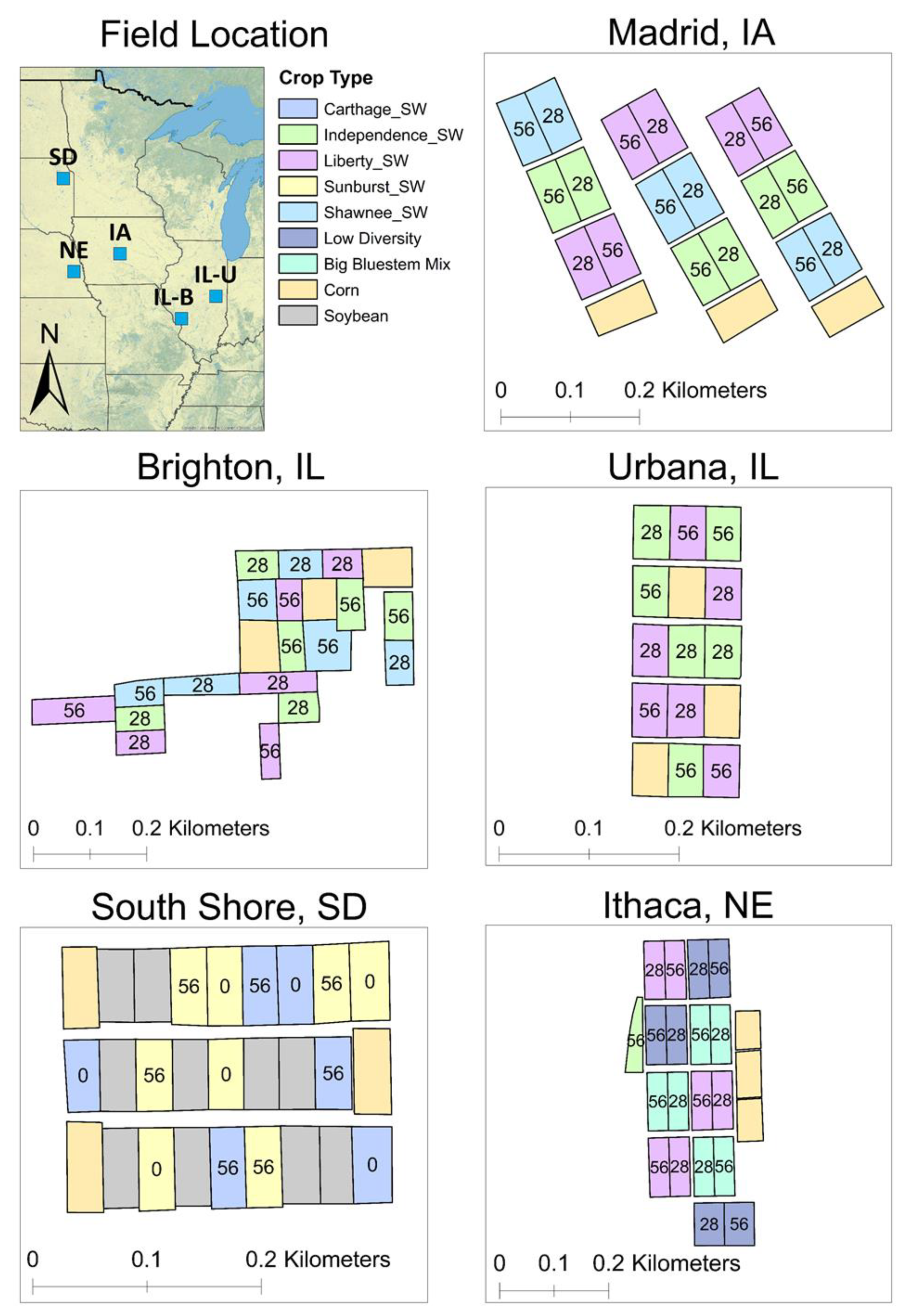
Figure 1. Field site locations in the U.S. Midwest and the plot layouts across the Brighton, Illinois (IL); Urbana, IL; Madrid, Iowa (IA); Ithaca, Nebraska (NE); and South Shore, South Dakota (SD) sites. Plots are labeled by crop/cultivar type (SW = switchgrass, Panicum virgatum L.) and annual nitrogen application (0, 28, or 56 kg N ha−1). The big bluestem (Andropogon gerardii Vitman) mixture includes ‘Goldmine’ and ‘Bonanza’ big bluestem cultivars. The low diversity mixture includes side-oats grama (Bouteloua curtipendula (Michx.) Torr.), Indiangrass (Sorghastrum nutans), and big bluestem.
Land 10 01221 g001
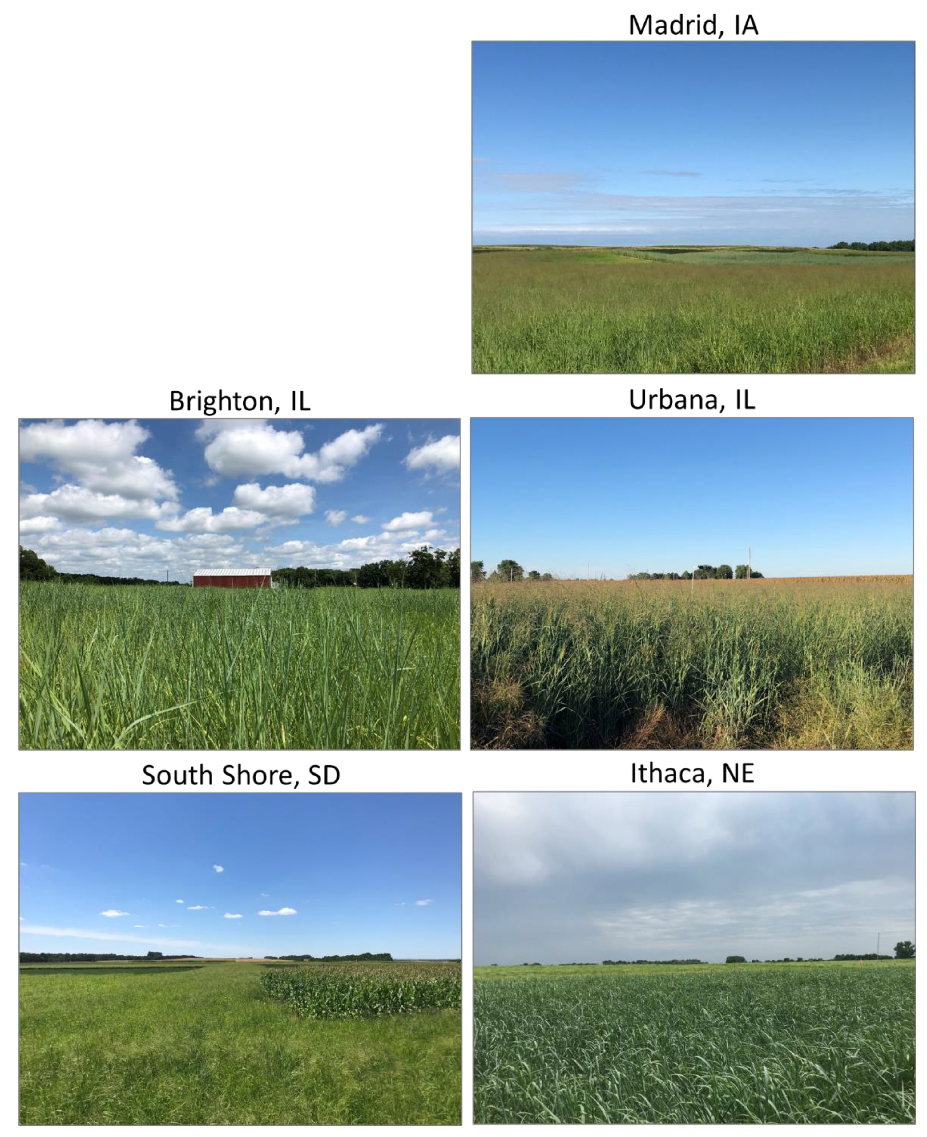
Figure 2. Photos of the study sites. The Brighton, Illinois (IL), and Urbana, IL, sites show ‘Independence’ switchgrass (SW) from July 2020 and September 2020, respectively. The Madrid, Iowa (IA), site shows ‘Shawnee’ SW foreground, Independence SW in the middle, and ‘Liberty’ SW in the top right before the tree line (July 2020). The Ithaca, Nebraska (NE), site shows Independence SW in the foreground and a low diversity mixture in the background (June 2020). The South Shore, South Dakota (SD), site shows ‘Sunburst’ SW as a border, corn on the left, and ‘Carthage’ SW and a soybean on the right (July 2020).
Land 10 01221 g002
Figure 3. Sentinel-2 multispectral imagery of the study sites displayed in true color. Brighton, Illinois (IL) (day-of-year (DOY) 169); Urbana, IL (DOY 281); Madrid, Iowa (IA) (DOY 177); Ithaca, Nebraska (NE) (DOY 165); and South Shore, South Dakota (SD) (DOY 193).
Land 10 01221 g003
Figure 4. Seasonal trajectories of the green normalized difference vegetation index (GNVDI) by switchgrass cultivars and mixed tallgrass between April and October 2020 across the (a) Brighton, Illinois (IL); (b) Urbana, IL; (c) Madrid, Iowa (IA); (d) Ithaca, Nebraska (NE); and (e) South Shore, South Dakota (SD), sites. Plot legends are named based on the combination of plot number, cultivar planted, and nitrogen (N) fertilization rate (kg N ha−1). Switchgrass (SW) cultivars: Lib = ‘Liberty’ SW, Shaw = ‘Shawnee’ SW, Indp = ‘Independence’ SW, Cart = ‘Carthage’ SW, and Sunb = ‘Sunburst’ SW. Mixed tallgrass: LD = low diversity mixture, BB = big bluestem mixture. DOY = day-of-year.
Land 10 01221 g004
Figure 5. Scatter plots of perennial grass yield measured at harvest and the green normalized difference vegetation index (GNDVI) on the dates having the highest correlation with yields across the (a) Brighton, Illinois (IL); (b) Urbana, IL; (c) Madrid, Iowa (IA); (d) Ithaca, Nebraska (NE); and (e) South Shore, South Dakota (SD), sites.
Land 10 01221 g005aLand 10 01221 g005b
Figure 6. Examples of scatter plots of measured switchgrass yields and switchgrass yields predicted based on the linear regression model output using the green normalized difference vegetation index across the (a) Brighton, Illinois (IL); (b) Urbana, IL; (c) Madrid, Iowa (IA); (d) Ithaca, Nebraska (NE); and (e) South Shore, South Dakota (SD), sites.
Land 10 01221 g006aLand 10 01221 g006b
Figure 7. Examples of switchgrass dry biomass yield (Mg/ha) for the five study sites.
Land 10 01221 g007
Table 1. Field site characteristics and crop management.
SiteCoordinatesField Size (Plot Size) (ha)Rainfall + Snow Melt * (mm)Cropping HistoryPlanting DateHarvest Date
Brighton, IL39°3′23.23″ N, 90°11′7.62″ W8.5 (0.4)1158 Corn/soybean rotation28 May 20199 December 2020
Urbana, IL40°4′7.68″ N, 88°11′26.78″ W6.1 (0.2)731Perennial grass plots
Soybean (2018)
Corn (2019)
30 May 20207 December 2020
Madrid, IA41°55′52.17″ N, 93°45′49.28″ W8.5 (0.4)730 Corn/soybean rotation13 June 201920 November 2020
Ithaca, NE41°8′57.54″ N, 96°27′14.07″ W8.9 (0.4)467 £Corn/soybean rotation14 June 2019
(‘Independence’)
18 April 2012
16 November 2020
South Shore, SD45°6′20.30″ N, 97°3′42.41″ W3.6 (0.2)533 Wheat/soybean rotation(all other grasses)
3 June 2019
19 November 2020
* Average of 2019 and 2020. Data provided by [47]. £ Data provided by [48]. Data provided by [49]. Data provided by [50].
Table 2. Summary of perennial grass yield data available for model development.
SitePlot
Count
Yield (Mg/ha)
Min., Max. (Range)MeanStandard Deviation
Brighton, IL182.27, 5.75 (3.48)4.201.45
Urbana, IL121.19, 4.35 (3.16)2.240.82
Madrid, IA182.45, 7.01 (4.56)4.621.86
Ithaca, NE19 14.14, 11.1 (6.96)7.751.67
South Shore, SD125.74, 10.4 (4.66)8.161.59
1 The single ‘Independence’ plot was excluded from the model development; thus 18 plots were used for the model development. Min. = minimum, Max. = maximum.
Table 3. Summary of imagery considered for model development.
SiteAprilMayJuneJulyAugustSeptemberOctoberTotal
Brighton, IL8, 18232, 7, 12, 17no image6, 165, 20, 25no image12
Urbana, IL5, 10, 20no image1414, 24, 298, 18, 23no image711
Madrid, IA1, 1266, 15, 2510193, 13, 18no image11
Ithaca, NE9, 19193, 8, 138, 13, 1817, 279, 16614
South Shore, SD7, 222, 271, 11, 1611, 1610, 254, 14no image13
Table 4. Spectral vegetation indices examined in this study.
IndexFormulaSource
Atmospherically resistant vegetation index (ARVI)[NIR − (R − B)]/[NIR + (R − B)] [51]
Difference vegetation index (DVI)NIR − R[52]
Enhanced vegetation index (EVI)2.5 × [(NIR − R)/(NIR + 6 × R − 7.5 × B + 1)][53]
Enhanced vegetation index 2 (EVI2)2.5 × [(NIR − R)/(NIR + 2.4 × R + 1)][54]
Green atmospherically resistant index (GARI){NIR − [G − 1.7 × (B − R)]}/{NIR + [G − 1.7 × (B − R)]}[55]
Green chlorophyll index (GCI)NIR/G − 1[56]
Green difference vegetation index (GDVI)NIR − G[57]
Green normalized difference vegetation index (GNDVI)(NIR − G)/(NIR + G)[58,59]
Green red ratio vegetation index (GRVI)G/R[60]
Infrared percentage vegetation index (IPVI)NIR/(NIR + R)[61]
Modified non-linear index (MNLI)[(NIR2 − R) × (1 + 0.5)]/(NIR2 + R + 0.5)[62]
Modified soil-adjusted vegetation index (MSAVI){2 × NIR + 1 − sqrt [(2 × NIR + 1)2 − 8 × (NIR − R)]}/2[63]
Modified simple ratio (MSR)[(NIR/R) − 1]/{[sqrt(NIR/R)] + 1}[64]
Normalized difference vegetation index (NDVI)(NIR − R)/(NIR + R)[65]
Optimized soil-adjusted vegetation index (OSAVI)(NIR − R)/(NIR + R + 0.16)[66]
Renormalized difference vegetation index (RDVI)(NIR − R)/[sqrt(NIR + R)][67]
Soil-adjusted vegetation index (SAVI)(1 + 0.5) × [(NIR − R)/(NIR + R + 0.5)][68]
Simple ratio (SR)NIR/R[69]
Visible atmospherically resistant index (VARI)(G − R)/(G + R − B)[70]
Wide dynamic range vegetation index (WDRVI)(0.2 × NIR − R)/(0.2 × NIR + R)[71]
B = blue band, G = green band, R = red band, and NIR = near-infrared band that correspond to bands 2, 3, 4, and 8 of Sentinel-2 satellite imagery, respectively; sqrt = square root.
Table 5. Summary of the highest coefficient of determination (R2) values between spectral vegetation indices and perennial grass dry biomass yields measured at harvest and the corresponding date of image collection for each study site *.
Spectral IndexSpectral Band Used in IndexBrighton, ILUrbana, ILMadrid, IAIthaca, NESouth Shore, SD
BGRNIRDOYR2DOYR2DOYR2DOYR2DOYR2
ARVIx xx1540.6602810.5591770.7132300.7182480.813
EVIx xx1540.6402810.6331770.7152300.7282480.839
EVI2 xx1540.6242810.7061770.7281650.8102230.802
GARIxxxx1540.6142810.6961770.6491650.8401930.909
GCI x x1690.5152810.8281920.7391650.8841930.878
GDVI xx2290.4512810.6261920.6361650.8692080.932
GLIxx x1540.622960.6141770.6481650.5762380.428
GNDVI x x1690.6052810.8421770.7761650.8731930.857
GRRVI xx 1540.553960.6141770.6201650.6382380.628
IPVI xx1540.6432810.6811770.7371650.8032230.800
MNLI xx1540.6372810.6591770.7251950.7722080.887
MSAVI xx1540.6612810.6471770.7381650.7952230.797
MSR xx1540.5322810.7432620.0701650.8272480.820
NDVI xx1540.6432810.6811770.7311650.8032230.800
OSAVI xx1540.6432810.6811770.7371650.8032230.800
RDVI xx1540.5272810.7161770.6801650.8412080.910
SAVI xx1540.6432810.6811770.7371650.8032230.800
SR xx1540.4842810.7521770.6481650.8262480.829
VARIxxx 1540.593960.6171770.6851650.6412380.639
WDRVI xx1540.5972810.7271770.7231650.8182230.805
* Three indices having the highest R2 with the switchgrass dry biomass yields are shown in boldface. More than three indices are indicated for the Brighton site because of the equal R2 values. DOY = day-of-year.
Table 6. Performance of linear regression models using the green normalized difference vegetation index 1 and characteristics of perennial grass dry biomass yield data used for model development.
SiteImage Date (DOY)R2MAERMSE
Brighton, IL1690.5920.5890.685
Urbana, IL2810.6940.3770.399
Madrid, IA1770.8350.5550.645
Ithaca, NE1650.8700.5390.616
South Shore, SD1930.8790.5790.653
1 The summary was generated from 31 iterations for each site. DOY = day-of-year; R2 = coefficient of determination; MAE = mean absolute error; RMSE = root mean squared error.
Publisher’s Note: MDPI stays neutral with regard to jurisdictional claims in published maps and institutional affiliations.