
Land Use Demands for the CLUE-S Spatiotemporal Model in an Agroforestry Perspective


 , ,
, ,
Abstract
:1. Introduction
2. Scenarios on Land Use Demands
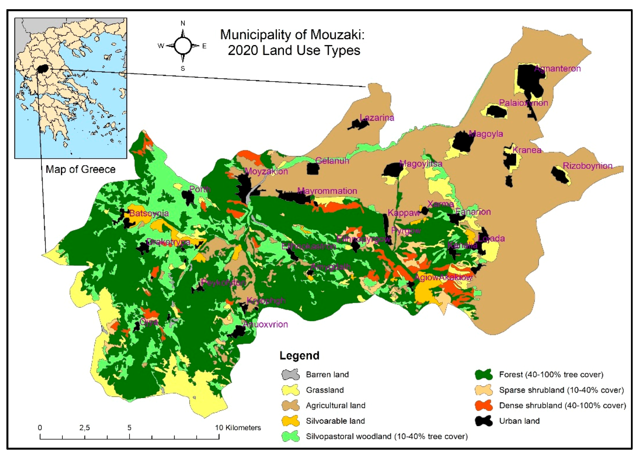
3. Study Area and Forecast Period
4. Materials and Methods
4.1. Business as Usual (BAU) Scenario
4.2. Rapid Economic Development (RED) Scenario
4.2.1. Parameters Estimation
4.2.2. Constraints on the Optimization Model
- C4: 10,343.15 ≤ x1 ≤ 11,144.03
- C5: 556.38 ≤ x2 ≤885.53
- C6: 1988.21 ≤ x3 ≤2405.00
- C7: 3815.39 ≤ x4 ≤4465.02
- C8: 10,573.64 ≤ x5 ≤ 14,249.39
- C9: 503.74 ≤ x6 ≤ 550.03
- C10: 608.97 ≤ x7 ≤ 784.99
- C11: 1457.79 ≤ x8 ≤ 1725.68
- C12: 0 ≤ x9 ≤ 86.01
4.3. Ecological Land Protection (ELP) Scenario
4.4. Multiobjective Optimization
5. Results
5.1. Results for the Three Scenarios BAU, RED, ELP
5.2. Trade-Offs between Economic and Ecological Benefits
6. Conclusions
Author Contributions
Funding
Institutional Review Board Statement
Informed Consent Statement
Data Availability Statement
Acknowledgments
Conflicts of Interest
References
- Ambarli, D.; Vrahnakis, M.; Burrascano, S.; Naqinezhad, A.; Pulido Fernández, M. Grasslands of the Mediterranean Basin and the Middle East and their management. In Grasslands of the World: Diversity, Management and Conservation; Squires, V.R., Dengler, J., Feng, H., Hua, L., Eds.; CRC Press: Boca Raton, FL, USA, 2018; ISBN 9781498796262. [Google Scholar]
- Guarino, R.; Vrahnakis, M.; Rodriguez Rojo, M.P.; Giouga, L.; Pasta, S. Grasslands and shrublands of the Mediterranean region. In Encyclopedia of the World’s Biomes. Volume 3: Forests—Trees of Life; Goldstein, M.I., DellaSala, D.A., DiPaolo, D.A., Eds.; Grasslands and Shrublands—Sea of Plants; Elsevier: Amsterdam, NL, USA, 2020; ISBN 978-012-8160-96-1. [Google Scholar]
- Chouvardas, D. Estimation of Diachronic Effects of Pastoral Systems and Land Uses in Landscapes with the Use of Geographic Information Systems (GIS). Ph.D. Thesis, School of Forestry and Natural Environment, Aristotle University of Thessaloniki, Thessaloniki, Greece, 2007. [Google Scholar]
- Papanastasis, V.P. Land use changes. In Mediterranean Mountain Environment; Vogiatzakis, I., Ed.; John Wiley & Sons Ltd.: Hoboken, NJ, USA, 2012; pp. 159–184. [Google Scholar]
- Chouvardas, D.; Ispikoudis, I.; Mitka, K.; Evangelou, C.; Papanastasis, V.P. Diachronic evolution of land use/ cover changes in pastoral landscapes of Greece. In Dry Grasslands of Europe: Grazing and Ecosystem Services; Vrahnakis, M., Kyriazopoulos, A.P., Chouvardas, D., Fotiadis, G., Eds.; Hellenic Range and Pasture Society: Thessaloniki, Greece, 2013; pp. 277–282. [Google Scholar]
- Perpiña, C.; Kavalov, B.; Diogo, V.; Jacobs-Crisioni, C.; Batista e Silva, F.; Lavalle, C. Agricultural Land Abandonment in the EU within 2015–2030; European Commission 2018; Joint Research Centre (Seville Site): Seville, Spain, 2018; p. JRC113718. [Google Scholar]
- Vrahnakis, M.; Nasiakou, S.; Kazoglou, Y.; Blanas, G. Business model for agroforestry consulting company. Agrofor. Syst. 2016, 90, 219–236. [Google Scholar] [CrossRef]
- Mwase, W.; Sefasi, A.; Njoloma, J.; Nyoka, B.I.; Manduwa, D.; Nyaika, J. Factors affecting the adoption of Agroforestry and evergreen agriculture in southern Africa. Environ. Nat. Resour. Res. 2015, 5, 148–157. [Google Scholar] [CrossRef] [Green Version]
- Adesina, A.; Chianu, J.N. Determinants of farmers’ adoption and adaptation of alley farming technology in Nigeria. Agrofor. Syst. 2002, 55, 99–112. [Google Scholar] [CrossRef]
- Fischer, A.; Vasseur, L. Smallholder perceptions of agroforestry projects in Panama. Agrofor. Syst. 2002, 54, 103–113. [Google Scholar] [CrossRef]
- Neupane, R.P.; Sharma, K.R.; Thapa, G.B. Adoption of agroforestry in the hills of Nepal: A logistic regression analysis. Agric. Syst. 2002, 72, 177–196. [Google Scholar] [CrossRef]
- Bannister, M.E.; Nair, P.K.R. Agroforestry adoption in Haiti: The importance of household and farm characteristics. Agrofor. Syst. 2003, 57, 149–157. [Google Scholar] [CrossRef]
- Djalilov, B.M.; Khamzina, A.; Hornidge, A.-K.; Lamers, J.P.A. Exploring constraints and incentives for the adoption of agroforestry practices on degraded cropland in Uzbekistan. J. Environ. Plan. Manag. 2015, 59, 142–162. [Google Scholar] [CrossRef]
- Marra, M.C.; Pannell, D.J.; Amir, A.G. The economics of risk, uncertainty and learning in the adoption of new agricultural technologies: Where are we on the learning curve? Agric. Syst. 2003, 75, 215–234. [Google Scholar] [CrossRef]
- Verburg, P.H.; Schot, P.; Dust, M.; Veldkamp, A. Land use change modelling: Current practice and research priorities. GeoJournal 2004, 64, 309–324. [Google Scholar] [CrossRef]
- Xiang, W.-N.; Clarke, K.C. The use of scenarios in land-use planning. Environ. Plan. B Plan. Des. 2003, 30, 885–909. [Google Scholar] [CrossRef] [Green Version]
- Shearer, A. Approaching scenario-based studies: Three perceptions about the future and considerations for landscape planning. Environ. Plan. B Plan. Des. 2005, 32, 67–87. [Google Scholar] [CrossRef]
- Veldkamp, A.; Lambin, E.F. Predicting Land Use Change. Agric. Ecosyst. Environ. 2001, 85, 1–6. [Google Scholar] [CrossRef]
- Verburg, P.H.; Soepboer, W.; Veldkamp, A.; Limpiada, R.; Espaldon, V.; Mastura, S. Modeling the spatial dynamics of regional land use: The CLUE-S model. Environ. Manag. 2002, 30, 391–405. [Google Scholar] [CrossRef]
- Chouvardas, D.; Vrahnakis, M.S. A semi-empirical model for the near-future evolution of the lake Koronia landscape. J. Environ. Prot. Ecol. 2009, 10, 867–876. [Google Scholar]
- Zhang, P.; Liu, Y.; Pan, Y.; Yu, Z. Land use pattern optimization based on CLUE-S and SWAT models for agricultural non-point source pollution control. Math. Comput. Model. 2013, 58, 558–595. [Google Scholar] [CrossRef]
- Han, H.; Yang, C.; Song, J. Scenario Simulation and the Prediction of Land Use and Land Cover Change in Beijing, China. Sustainability 2015, 7, 4260–4279. [Google Scholar] [CrossRef] [Green Version]
- Reginster, I.; Rounsevel, M. Scenarios of future urban land use in Europe. Environ. Plan. B Urban Anal. City Sci. 2006, 33, 619–636. [Google Scholar] [CrossRef]
- Hoymann, J. Quantifying demand for built-up area—A comparison of approaches and application to regions with stagnating population. J. Land Use Sci. 2012, 7, 67–87. [Google Scholar] [CrossRef]
- Wang, Y.; Li, X.; Zhang, Q.; Li, J.; Zhou, X. Projections of future land use changes: Multiple scenarios-based impacts analysis on ecosystem services for Wuhan city, China. Ecol. Indic. 2018, 94, 430–445. [Google Scholar] [CrossRef]
- Nasiakou, S.; Chouvardas, D.; Vrahnakis, M.; Kleftoyianni, V. Temporal changes analysis of Mouzaki’s landscape, western Thessaly, Greece (1960–2020). In Proceedings of the 10th Panhellenic Rangeland Congress of the Hellenic Range and Pasture Society, Florina, Greece, 2021; p. 6, in press. (In Greek with English Summary). [Google Scholar]
- HSA. State’s Statistical Data; Hellenic Statistic Authority: Athens, Greece, 2018. [Google Scholar]
- Mantzanas, K. Forest Species with Short Rotation Time and Agroforestry. In Forest Wood Species Plantations of Short Rotation Time for Biomass Production and Thermal Uses; Centre for Renewable Energy Sources and Saving (CRES), Department of Biomass, AGROTICA: Thessaloniki, Greece, 2016. [Google Scholar]
- Albanis, Κ.; Xanthopoulos, G.; Skouteri, A.; Theodoridis, N.; Christodoulou, A.; Palaskas, D. Methodology for Estimating the Value of Forest Land in Greece—Detailed Manual; Institute of Mediterranean Forest Ecosystems and Forest Products Technology, Ministry of Environment and Energy: Athens, Greece, 2015.
- Costanza, R.; d’Arge, R.; de Groot, R.; Farberk, S.; Grasso, M.; Hannon, B.; Limburg, K.; Naeem, S.; O’Neill, R.V.; Paruelo, J.; et al. The value of the world’s ecosystem services and natural capital. Nature 1997, 387, 253–260. [Google Scholar] [CrossRef]

| Variable | Land Use Type | Area in 1960 (Ha) | Area in 2020 (Ha) | Difference (%) | Predicted Area in 2040 (Ha) |
|---|---|---|---|---|---|
| x1 | Agricultural land | 14,206.52 | 11,144.03 | −21.56 | 10,343.15 |
| x2 | Silvoarable land | 200.51 | 556.38 | 177.48 | 650.26 |
| x3 | Grassland | 5009.69 | 2405 | −51.99 | 1988.21 |
| x4 | Silvopastoral woodland (10–40% tree cover) | 2525.42 | 3815.39 | 51.08 | 4000.68 |
| x5 | Forest (40–100% tree cover) | 5175.8 | 10,573.64 | 104.29 | 11,622.04 |
| x6 | Sparse shrubland (10–40% cover) | 394.88 | 503.74 | 27.57 | 516.94 |
| x7 | Dense shrubland (40–100% cover) | 2398.44 | 784.99 | −67.27 | 608.97 |
| x8 | Urban land | 939.72 | 1457.79 | 55.13 | 1534.20 |
| x9 | Barren land | 475.99 | 86.01 | −81.93 | 62.52 |
| TOTAL: | 31,326.97 | 31,326.97 | - | 31,326.97 | |
| Services and Externalities | Fir | Spruce | Pine | Beech | Oak | Total |
|---|---|---|---|---|---|---|
| Total area (Ha) | 548,070 | 2754 | 878,786 | 336,640 | 470,989 | 2,237,239 |
| Wood production (×106 €) | 29.06 | 0.72 | 27.96 | 15.22 | 12.67 | 85.63 |
| Non-Wood Forest Products (×106 €) | ||||||
| Mushroom | 0.82 | 0.42 | 0.50 | 0.71 | 2.45 | |
| Honey | 5.61 | 0.028 | 9.00 | 3.45 | 15.07 | 33.16 |
| Christmas trees | 0.62 | 0.62 | ||||
| Resin | 9.58 | 9.58 | ||||
| Pine seeds | 0.55 | 0.55 | ||||
| Total (NTFPs) | 7.05 | 0.03 | 19.55 | 3.95 | 15.78 | 46.36 |
| Livestock grazing (×106 €) | 16.63 | 0.08 | 26.89 | 10.30 | 0.00 | 53.90 |
| Hunting (×106 €) | 0.54 | 0.00 | 0.86 | 0.33 | 0.46 | 2.19 |
| Recreation (×106 €) | 51.68 | 0.26 | 82.87 | 31.75 | 44.41 | 210.97 |
| Soil protection (×106 €) | 57.55 | 0.29 | 92.270 | 35.35 | 103.03 | 288.49 |
| C sequestration (×106 €) | 2.86 | 0.017 | 5.69 | 2.19 | 3.01 | 13.77 |
| Biodiversity (×106 €) | 46.04 | 0.23 | 73.82 | 28.28 | 39.56 | 187.93 |
| Losses (wildfires) (×106 €) | 21.18 | 0.12 | 48.64 | 12.43 | 46.03 | 128.40 |
| Total annual value (×106 €) | 190.23 | 1.52 | 281.27 | 114.94 | 172.89 | 760.85 |
| Variable | Land Use Type | Annual Financial Benefit (€/Ha) |
|---|---|---|
| x1 | Agricultural land | 3146.10 |
| x2 | Silvoarable land | 3914.55 |
| x3 | Grassland | 306.74 |
| x4 | Silvopastoral woodland (10–40% tree cover) | 278.64 |
| x5 | Forest (40–100% tree cover) | 340.08 |
| x6 | Sparse shrubland (10–40% cover) | 511.68 |
| x7 | Dense shrubland (40–100% cover) | 188.3 |
| x8 | Urban land | 45,038.35 |
| x9 | Barren land | 0.0 |
| Services and Externalities | Grassland | Silvopastoral Woodland | Sparse Shrubland | Dense Shrubland |
|---|---|---|---|---|
| Total area (Ha) | 1,000,000 | 1,000,850 | 1,309,992 | 1,964,987 |
| Wood production (×106 €) | 12.67 | 1.508 | 2.262 | |
| Mushrooms (×106 €) | 1.50 | 0.035 | 0.015 | |
| Honey (×106 €) | 10.24 | 10.25 | 20.118 | 13.412 |
| Heath (Erica) roots (x 106) | 0.004 | 0.002 | ||
| Livestock grazing (×106 €) | 125.00 | 45.04 | 211.128 | 52.782 |
| Hunting (×106 €) | 0.98 | 0.98 | 2.240 | 0.960 |
| Recreation (×106 €) | 91.00 | 94.38 | 199.376 | 49.840 |
| Soil protection (×106 €) | 67.98 | 51.51 | 68.776 | 275.100 |
| C sequestration (×106 €) | 1.22 | 1.50 | 1.148 | 1.720 |
| Biodiversity (×106 €) | 48.00 | 84.07 | 220.080 | 55.020 |
| Losses (wildfires) (×106 €) | 37.68 | 23.02 | 54.112 | 81.170 |
| Total annual value (×106 €) | 306.74 | 278.88 | 670.301 | 369.955 |
| Variable | Land Use Type | Annual Financial Benefit (€/Ha) |
|---|---|---|
| x1 | Agricultural land | 67.75 |
| x2 | Silvoarable land | 178.94 |
| x3 | Grassland | 170.84 |
| x4 | Silvopastoral woodland (10–40% tree cover) | 196.61 |
| x5 | Forest (40–100% tree cover) | 222.38 |
| x6 | Sparse shrubland (10–40% cover) | 170.84 |
| x7 | Dense shrubland (40–100% cover) | 170.84 |
| x8 | Urban land | 0.0 |
| x9 | Barren land | 0.0 |
| Variable | Land Use Type | Estimated Area in 2040 (Ha) | ||
|---|---|---|---|---|
| BAU | RED | ELP | ||
| x1 | Agricultural land | 10,343.15 | 11,144.03 | 10,343.15 |
| x2 | Silvoarable land | 650.26 | 885.53 | 556.38 |
| x3 | Grassland | 1988.21 | 2026.21 | 1988.21 |
| x4 | Silvopastoral woodland (10–40% tree cover) | 000.68 | 3815.39 | 3815.39 |
| x5 | Forest (40–100% tree cover) | 11,622.04 | 10,617.45 | 12,053.37 |
| x6 | Sparse shrubland (10–40% cover) | 516.94 | 541.71 | 503.74 |
| x7 | Dense shrubland (40–100% cover) | 608.97 | 608.97 | 608.97 |
| x8 | Urban land | 1534.2 | 1725.68 | 1457.79 |
| x9 | Barren land | 62.52 | 0 | 0 |
| TOTAL | 31,326.97 | 31,326.97 | 31,326.97 | |
| Variable | Land Use Type | Estimated Area in 2040 (Ha) |
|---|---|---|
| RED | ||
| x1 | Agricultural land | 10,343.15 |
| x2 | Silvoarable land | 1768.22 |
| x3 | Grassland | 1988.21 |
| x4 | Silvopastoral woodland (10–40% tree cover) | 3815.39 |
| x5 | Forest (40–100% tree cover) | 10,573.64 |
| x6 | Sparse shrubland (10–40% cover) | 503.74 |
| x7 | Dense shrubland (40–100% cover) | 608.97 |
| x8 | Urban land | 1725.68 |
| x9 | Barren land | 0 |
| TOTAL | 31,326.97 | |
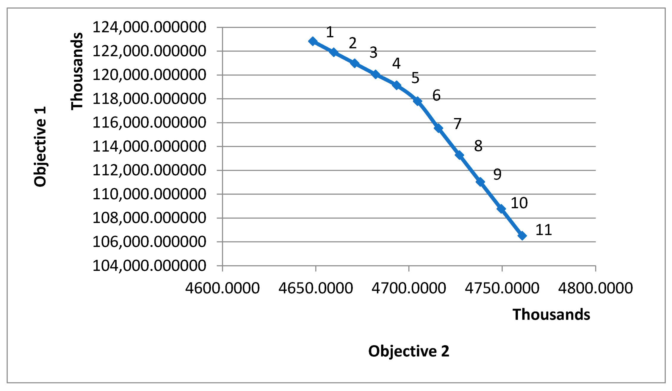
| Point 1 | Point 2 | Point 3 | Point 4 | Point 5 | Point 6 | Point 7 | Point 8 | Point 9 | Point 10 | Point 11 | |
|---|---|---|---|---|---|---|---|---|---|---|---|
| X1 | 10,343.15 | 10,343.15 | 10,343.15 | 10,343.15 | 10,343.15 | 10,343.15 | 10,343.15 | 10,343.15 | 10,343.15 | 10,343.15 | 10,343.15 |
| X2 | 1768.19 | 1509.88 | 1251.56 | 993.23 | 734.91 | 556.38 | 556.38 | 556.38 | 556.38 | 556.38 | 556.38 |
| X3 | 1988.21 | 1988.21 | 1988.21 | 1988.21 | 1988.21 | 1988.21 | 1988.21 | 1988.21 | 1988.21 | 1988.21 | 1988.21 |
| X4 | 3815.39 | 3815.39 | 3815.39 | 3815.39 | 3815.39 | 3815.39 | 3815.39 | 3815.39 | 3815.39 | 3815.39 | 3815.39 |
| X5 | 10,573.64 | 10,831.95 | 11,090.27 | 11,348.60 | 11,606.92 | 11,801.04 | 11,851.50 | 11,901.96 | 11,952.42 | 12,002.88 | 12,053.34 |
| X6 | 503,74 | 503.74 | 503.74 | 503.74 | 503.74 | 503.74 | 503.74 | 503.74 | 503.74 | 503.74 | 503.74 |
| X7 | 608.97 | 608.97 | 608.97 | 608.97 | 608.97 | 608.97 | 608.97 | 608.97 | 608.97 | 608.97 | 608.97 |
| X8 | 1725.68 | 1725.68 | 1725.68 | 1725.68 | 1725.68 | 1710.09 | 1659.63 | 1609.17 | 1558.71 | 1508.25 | 1457.79 |
| X9 | 0.00 | 0 | 0 | 0 | 0 | 0 | 0 | 0 | 0 | 0 | 0 |
| F1 | 122,825,300.00 | 121,902,000.00 | 120,978,600.00 | 120,055,300.00 | 119,131,900.00 | 117,797,100.00 | 115,541,500.00 | 113,286,000.00 | 111,030,500.00 | 108,775,000.00 | 106,519,500.00 |
| F2 | 4,648,419.00 | 4,659,640.50 | 4,670,862.00 | 4,682,083.50 | 4,693,305.00 | 4,704,526.50 | 4,715,748.00 | 4,726,969.50 | 4,738,191.00 | 4,749,412.50 | 4,760,634.00 |
Publisher’s Note: MDPI stays neutral with regard to jurisdictional claims in published maps and institutional affiliations. |
© 2021 by the authors. Licensee MDPI, Basel, Switzerland. This article is an open access article distributed under the terms and conditions of the Creative Commons Attribution (CC BY) license (https://creativecommons.org/licenses/by/4.0/).
Share and Cite
Mamanis, G.; Vrahnakis, M.; Chouvardas, D.; Nasiakou, S.; Kleftoyanni, V. Land Use Demands for the CLUE-S Spatiotemporal Model in an Agroforestry Perspective. Land 2021, 10, 1097. https://doi.org/10.3390/land10101097
Mamanis G, Vrahnakis M, Chouvardas D, Nasiakou S, Kleftoyanni V. Land Use Demands for the CLUE-S Spatiotemporal Model in an Agroforestry Perspective. Land. 2021; 10(10):1097. https://doi.org/10.3390/land10101097
Chicago/Turabian StyleMamanis, Georgios, Michael Vrahnakis, Dimitrios Chouvardas, Stamatia Nasiakou, and Vassiliki Kleftoyanni. 2021. "Land Use Demands for the CLUE-S Spatiotemporal Model in an Agroforestry Perspective" Land 10, no. 10: 1097. https://doi.org/10.3390/land10101097
APA StyleMamanis, G., Vrahnakis, M., Chouvardas, D., Nasiakou, S., & Kleftoyanni, V. (2021). Land Use Demands for the CLUE-S Spatiotemporal Model in an Agroforestry Perspective. Land, 10(10), 1097. https://doi.org/10.3390/land10101097