
Synthesizing Data to Classify and Risk Assess Vegetation Types for Regulations in Inland New South Wales Australia

Abstract
:1. Introduction
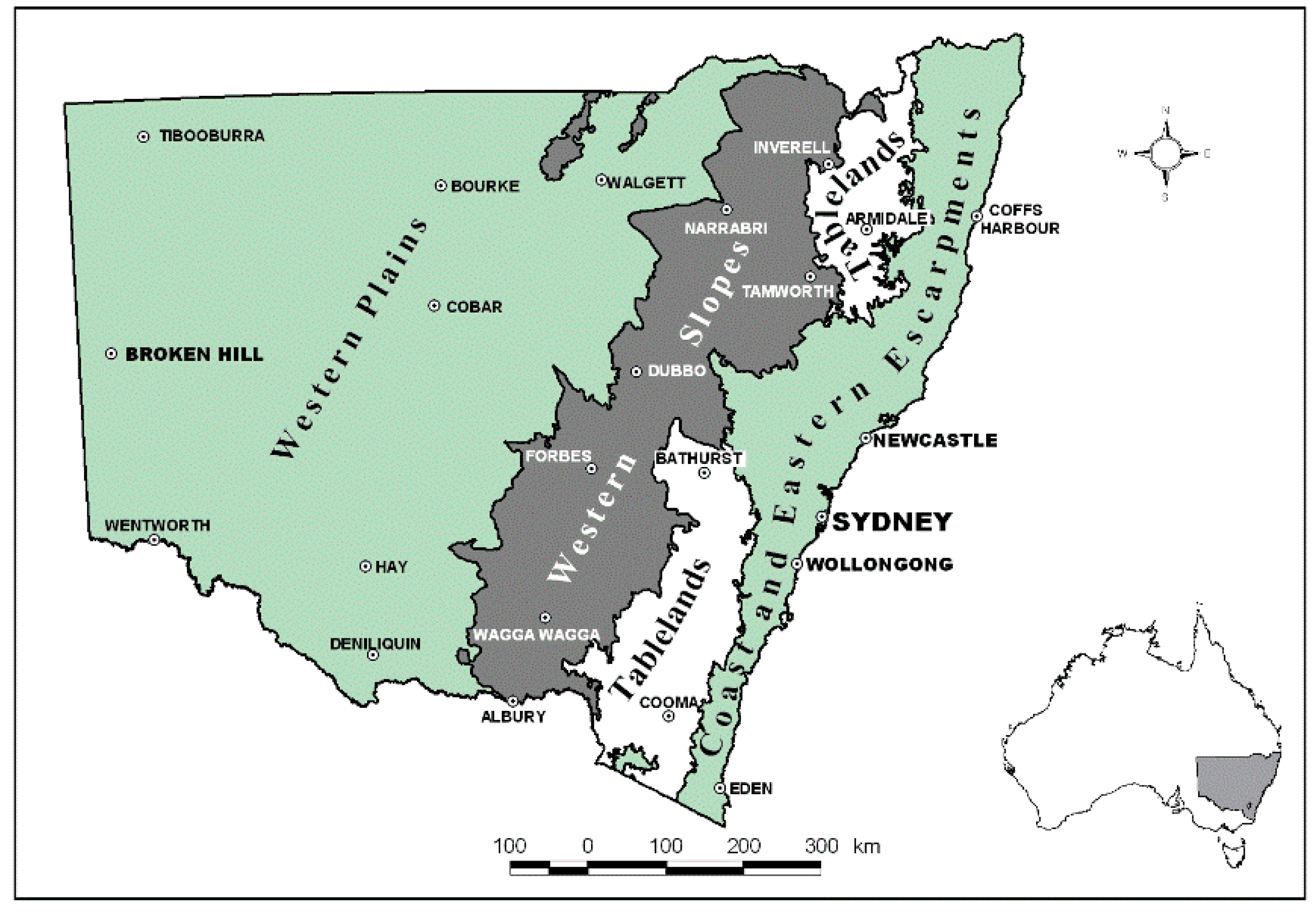
2. Study Area
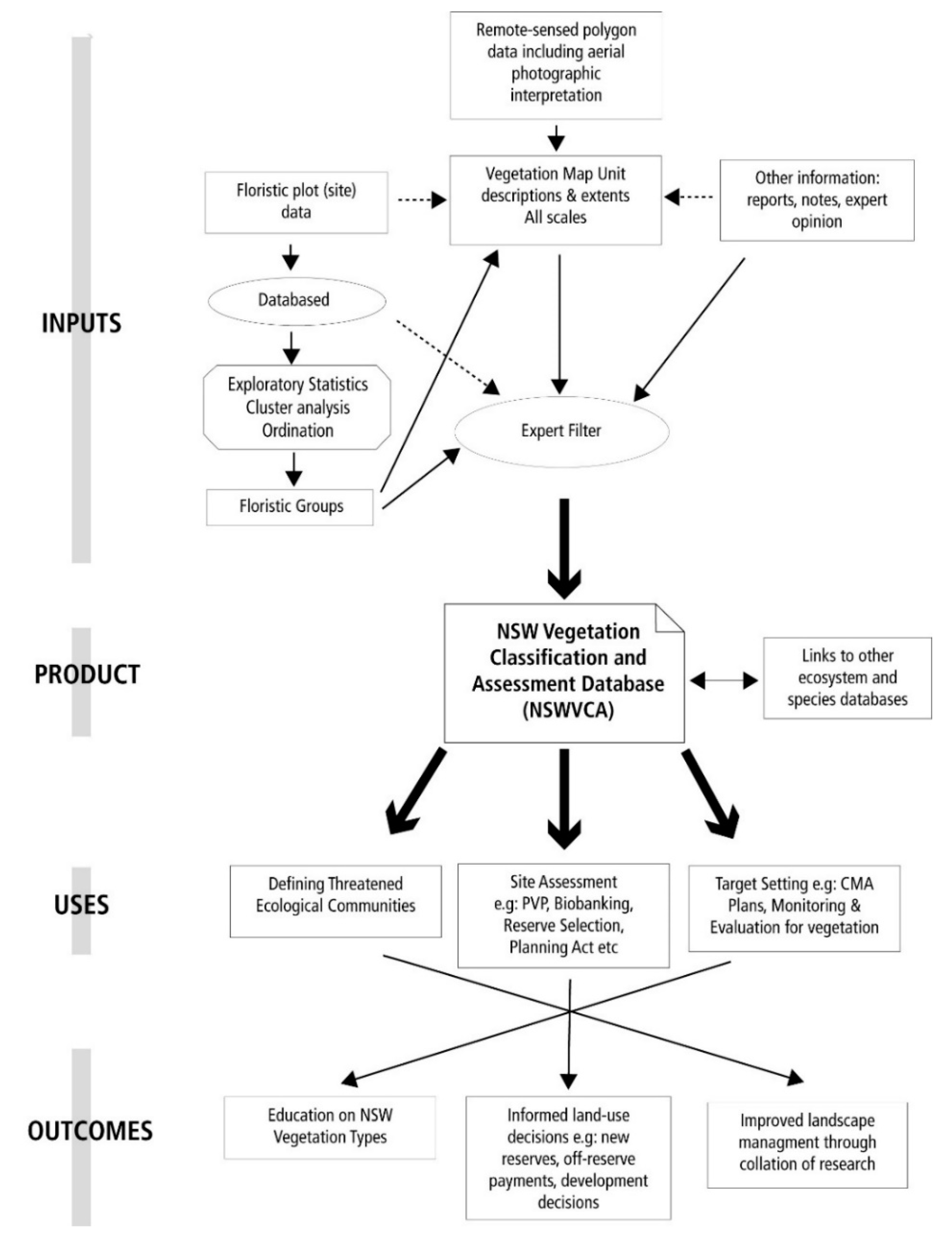
3. Methods
4. Results
5. Discussion
6. Conclusions
Supplementary Materials
Funding
Data Availability Statement
Acknowledgments
Conflicts of Interest
Abbreviations
| AOO | Area of Occurrence |
| CR | Critically Endangered |
| EN | Endangered |
| EOO | Extent of Occupancy |
| IUCN | World Conservation Union |
| IVC | International Vegetation Classification |
| LC | Least Concern |
| NSWVCA | New South Wales Vegetation Classification and Assessment Database |
| PA | Protected Area |
| PCT | Plant Community Type |
| PVP | Property Vegetation Plan |
| RLE | IUCN Red List of Ecosystems |
| TEC | Threatened Ecological Community listed under Australian law |
| NT | Near Threatened |
| VU | Vulnerable |
References
- Jones, M.B.; Schildhaurer, M.P.; Reichman, O.J.; Bowers, S. The new bioinformatics: Ecological data from the gene to the biosphere. Annu. Rev. Ecol. Evol. Syst. 2006, 37, 519–544. [Google Scholar] [CrossRef]
- Jax, K. Ecological Units: Definitions and Application. Q. Rev. Biol. 2006, 81, 237–258. [Google Scholar] [CrossRef]
- Comer, P.; Faber-Langendoen, D.; Evans, R.; Gawler, S.; Josse, C.; Kittel, G.; Menard, S.; Pyne, M.; Reid, M.; Schulz, K.; et al. Ecological Systems of the United States: A Working Classification of U.S. Terrestrial Systems; NatureServe: Arlington, VA, USA, 2003. [Google Scholar]
- Oliver, I. A framework and toolkit for scoring the biodiversity value of habitat, and the biodiversity condition within the context of biodiversity conservation. Ecol. Manag. Restor 2004, 5, 75–78. [Google Scholar] [CrossRef]
- BioMetric Version 1.8: A Terrestrial Biodiversity Assessment Tool for the NSW Property Vegetation Plan Developer Operational Manual. Available online: https://www.environment.nsw.gov.au/resources/pestsweeds/biometric_manual_1_8.pdf (accessed on 26 August 2021).
- NSW Ecosystems Study: Background and Methodology. Available online: https://www.environment.nsw.gov.au/resources/conservation/EcosystemsMethodology.pdf (accessed on 26 August 2021).
- Schmid, R.; Keith, D. From Ocean Shores to Desert Dunes: The Native Vegetation of New South Wales and the ACT. TAXON 2005, 54, 1120. [Google Scholar] [CrossRef]
- New South Wales Vegetation Classification and Assessment: Introduction—The Classification, Database, Assessment of Protected Areas and Threat Status of Plant Communities. Available online: https://www.rbgsyd.nsw.gov.au/getmedia/623f3dc8-99ba-421f-a909-638dc07e1064/Cun9Ben331.pdf.aspx (accessed on 26 August 2021).
- Beadle, N.C.W. The Vegetation of Australia; Cambridge University Press: Cambridge, UK, 1981. [Google Scholar]
- Grossman, D.H.; Faber-Langendoen, D.; Weakley, A.S.; Anderson, M.; Bourgeron, P.; Crawford, R.; Goodin, K.; Landaal, S.; Metzler, K.; Patterson, K.D.; et al. International Classification of Ecological Communities: Terrestrial Vegetation of the United States; The Nature Conservancy: Arlington, VA, USA, 1998. [Google Scholar]
- Beadle, N.C.W.; Costin, A.B. Ecological classification and nomenclature. Proc. Linn. Soc. NSW 1952, 67, 61–82. [Google Scholar]
- Faber-Langendoen, D.; Keeler-Wolf, T.; Meidinger, D.; Josse, C.; Weakley, A.; Tart, D.; Navarro, G.; Hoagland, B.; Ponomarenko, S.; Fults, G.; et al. Classification and Description of World Formation Types; RMRS-GTR-346; U.S. Department of Agriculture, Forest Service, Rocky Mountain Research Station: Fort Collins, CO, USA, 2016; 222p. [Google Scholar] [CrossRef]
- Dudley, N.; Stolton, S. (Eds.) Defining Protected Areas: An International Conference in Almeria, Spain; IUCN: Gland, Switzerland, 2008; 220p. [Google Scholar]
- Thackway, R.; Cresswell, I.D. An Interim Biogeographic Regionalisation for Australia; Version 6.0; Australian Nature Conservation Agency: Canberra, Australia, 1995. Available online: https://environment.gov.au/land/nrs/science/ibra (accessed on 26 August 2021).
- Benson, J.S.; Allen, C.; Togher, C.; Lemmon, J. New South Wales Vegetation Classification and Assessment: Part 1 Plant communities of the NSW Western Plains. Cunninghamia 2006, 9, 383–451. [Google Scholar]
- Benson, J.S. New South Wales Vegetation Classification and Assessment: Part 2 Plant communities in the NSW South-western Slopes Bioregion and update of NSW Western Plains plant communities. Version 2 of the NSWVCA database. Cunninghamia 2008, 10, 599–673. [Google Scholar]
- Benson, J.S.; Richards, P.; Waller, S.; Allen, C. New South Wales Vegetation Classification and Assessment: Part 3 Plant communities in the Brigalow Belt South, Nandewar and western New England Bioregions: Version 3 of the NSWVCA database. Cunninghamia 2010, 11, 457–579. [Google Scholar]
- IUCN. Red List Categories: Version 3.1; Prepared by the IUCN Species Survival Commission; IUCN: Gland, Switzerland; Cambridge, UK, 2001. [Google Scholar]
- Keith, D.A.; Rodríguez, J.P.; Rodriguez-Clark, K.; Nicholson, E.; Aapala, K.; Alonso, A.; Asmussen, M.; Bachman, S.; Basset, A.; Barrow, E.G.; et al. Scientific Foundations for an IUCN Red List of Ecosystems. PLoS ONE 2013, 8, e62111. [Google Scholar] [CrossRef] [Green Version]
- Bland, L.M.; Keith, D.A.; Miller, R.M.; Murray, N.J.; Rodríguez, J.P. (Eds.) Guidelines for the Application of IUCN Red List of Ecosystems Categories and Criteria, Version 1.1; IUCN: Gland, Switzerland, 2017. [Google Scholar]
- Andren, H. Effects of Habitat Fragmentation on Birds and Mammals in Landscapes with Different Proportions of Suitable Habitat: A Review. Oikos 1994, 71, 355–366. [Google Scholar] [CrossRef] [Green Version]
- Fahrig, L. Relative Effects of Habitat Loss and Fragmentation on Population Extinction. J. Wildl. Manag. 1997, 61, 603–610. [Google Scholar] [CrossRef]
- JANIS Joint ANZECC/MCFFA National Forest Policy Statement Implementation Sub-committee. Nationally Agreed Criteria for the Establishment of a Comprehensive, Adequate and Representative Reserve System for Forests in Australia; Commonwealth of Australia: Canberra, Australia, 1997. Available online: https://www.agriculture.gov.au/forestry/policies/rfa/about/protecting-environment (accessed on 26 August 2021).
- Braun-Blanquet, J. Plant Sociology: The Study of Plant Communities; Translated, revised and edited by Fuller, G.D.; Conrad, H.S. in 1983; Koeltz Scientific Books: Hesse, Germany, 1932. [Google Scholar]
- Poore, M.E.D. The Use of Phytosociological Methods in Ecological Investigations: III. Practical Application. J. Ecol. 1955, 43, 606–651. [Google Scholar] [CrossRef]
- Sivertsen, D. Native Vegetation Interim Type Standard; Department of Environment, Climate Change and Water: Sydney, Australia, 2009. Available online: https://www.environment.nsw.gov.au/-/media/OEH/Corporate-Site/Documents/Research/Maps-and-data/native-vegetation-interim-type-standard-100060.pdf (accessed on 26 August 2021).
- Belbin, L. The analysis of pattern in bio-survey data. In Nature Conservation: Cost Effective Biological Surveys and Data Analysis; Margules, C.R., Austin, M.P., Eds.; CSIRO: Canberra, Australia, 1991; pp. 176–190. [Google Scholar]
- Goodall, D.W. Objective classification of vegetation II. Fidelity and indicator value. Aust. J. Bot. 1953, 1, 434–456. [Google Scholar] [CrossRef]
- Hunter, J.T.; Hunter, V.H. Vegetation of Naree and Yantabulla stations on the Cuttaburra Creek, Far North Western Plains, New South Wales. Cunninghamia 2016, 16, 65–100. [Google Scholar] [CrossRef]
- Department of Planning, Industry and Environment NSW. BioNet Systematic Survey. Available online: https://www.environment.nsw.gov.au/research/VISplot.htm (accessed on 26 August 2021).
- Eco Logical Australia. NSW Vegetation Classification and Assessment (NSWVCA): Nandewar & Western New England Tablelands Bioregions; Project No. 174–001; Eco Logical Australia Pty Ltd.: Coffs Harbour, Australia, 2008. [Google Scholar]
- Australian Government Department of Agriculture, Water and Environment. EPBC Act, Threatened Ecological Communities in New South Wales and ACT. Available online: http://environment.gov.au/biodiversity/threatened/communities/NSW-ACT (accessed on 4 October 2021).
- NSW Government, Biodiversity Conservation Act NSW, Schedule 2, List of Threatened Ecological Communities. Available online: https://legislation.nsw.gov.au/view/html/inforce/current/act-2016-063#sch.2 (accessed on 26 August 2021).
- Department Planning, Infrastructure and Environment NSW. Bionet Vegetation Classification. Available online: https://www.environment.nsw.gov.au/research/Visclassification.htm (accessed on 4 October 2021).
- Gellie, N.J.H.; Hunter, J.T.; Benson, J.S.; Kirkpatrick, J.B.; Cheal, D.C.; McCreery, K.; Brocklehurst, P. Overview of plot-based vegetation classification approaches within Australia. Phytocoenologia 2018, 48, 251–272. [Google Scholar] [CrossRef]
- Geri, F.; La Porta, N.; Zottele, F.; Ciolli, M. Mapping Historical Data: Recovering a Forgotten Floristic and Vegetation Database for Biodiversity Monitoring. ISPRS Int. J. Geo-Inform. 2016, 5, 100. [Google Scholar] [CrossRef]
- Sattler, P.S.; Williams, R.D. (Eds.) The Conservation Status of Queensland’s Bioregional Ecosystems; Environmental Protection Agency: Brisbane, Australia, 1999. [Google Scholar]
- Gowans, S.; Milne, R.; Westbrooke, M.; Palmer, G. Survey of Vegetation in Tooralie; Prepared for the NSW Government Office for Environment & Heritage; Centre for Environmental Management University of Ballarat: Victoria, Australia, 2012. [Google Scholar]
- Westbrooke, M.; Gowans, S.; Gibson, M. The vegetation of the Coonavitra area, Paroo Darling National Park, western New South Wales. Cunninghamia 2011, 12, 7–27. [Google Scholar]
- Jennings, M.D.; Faber-Langendoen, D.; Loucks, O.L.; Peet, R.K.; Roberts, D. Standards for associations and alliances of the U.S. National Vegetation Classification. Ecol. Mono. 2009, 79, 173–199. [Google Scholar] [CrossRef]
- Benson, J.S. Sampling, strategies and costs of regional vegetation vegetation mapping. The Globe 1995, 43, 18–28. [Google Scholar]
- Berg, C.; Ewald, J.; Hobohm, C.; Dengler, J. The whole and its parts: Why and how to disentangle plant communities and synusiae in vegetation classification. Appl. Veg. Sci. 2019, 23, 127–135. [Google Scholar] [CrossRef] [Green Version]
- Hunter, J.T. Temporal phytocoenosia and synusiae: Should we consider temporal sampling in vegetation classification? Aust. J. Bot. 2021. [Google Scholar] [CrossRef]
- Faber-Langendoen, D.; Aaseng, N.; Hop, K.; Lew-Smith, M.; Drake, J. Vegetation classification, mapping, and monitoring at Voyageurs National Park, Minnesota: An application of the U.S. National Vegetation Classification. Appl. Veg. Sci. 2007, 10, 361–374. [Google Scholar] [CrossRef]
- Macquarie Marshes Adaptive Environment Management Plan: Synthesis of Information Projects and Actions; NSW Department of Environment Climate Change and Water: Sydney, Australia, 2010. Available online: https://www.environment.nsw.gov.au/-/media/OEH/Corporate-Site/Documents/Water/Water-for-the-environment/macquarie-marshes-adaptive-environmental-management-plan-100224.pdf (accessed on 26 August 2021).
- Gwydir Wetlands Adaptive Environment Management Plan: Synthesis of Information Projects and Actions; NSW Department of Environment Climate Change and Water: Sydney, Australia, 2010. Available online: https://www.environment.nsw.gov.au/-/media/OEH/Corporate-Site/Documents/Water/Water-for-the-environment/gwydir-wetlands-adaptive-environmental-management-plan-110027.pdf (accessed on 26 August 2021).
- Maguire, O.; Armstrong, R.; Benson, J.; Streeter, R.; Paterson, C.; McDonald, P.; Salter, N.; East, M.; Webster, M.; Sheahan, M.; et al. Using high resolution digital aerial imagery interpreted in a 3-D digital GIS environment to map predefined plant communities in central-southern New South Wales. Cunninghamia 2012, 12, 247–266. [Google Scholar] [CrossRef] [Green Version]
- Department of Planning, Industry and Environment NSW. State Vegetation Type Map. 2021. Available online: https://www.environment.nsw.gov.au/vegetation/state-vegetation-type-map.htm (accessed on 26 August 2021).
- Definiens Imaging GmbH eCognition User Guide 4; Definiens Imaging, GmbH: Munich, Germany, 2021; Available online: https://www.geospatialworld.net/news/the-new-ecognition-professional-4-0/ (accessed on 26 August 2021).
- Elith, J.; Leathwick, J.R.; Hastie, T. A working guide to boosted regression trees. J. Anim. Ecol. 2008, 77, 802–813. [Google Scholar] [CrossRef] [PubMed]
- Ferrier, S.; Guisan, A. Spatial modelling of biodiversity at the community level. J. Appl. Ecol. 2006, 43, 393–404. [Google Scholar] [CrossRef]
- Hunter, J.T. Validation of the Greater Hunter Native Vegetation Mapping as it pertains to the Upper Hunter region of New South Wales. Ecol. Manag. Restor. 2016, 17, 40–46. [Google Scholar] [CrossRef]
- Benson, J.S.; Ashby, E. The vegetation of the Guyra 1:100,000 map sheet New England Bioregion, New South Wales. Cunninghamia 2000, 6, 747–872. [Google Scholar]
- Brown, K. National Park Service vegetation inventory and use of hybrid approaches to signature development and object-oriented tools. In Proceedings of the PECORA 17—The Future of Land Imaging…Going Operational, Denver, CO, USA, 18–20 November 2008. [Google Scholar]
- Benson, J.S. Comprehensive, reliable vegetation classification and mapping is vital for terrestrial restoration ecology. In Restore, Regenerate, Revegetate: A Conference on Restoring Ecological Processes, Ecosystems and Landscapes in a Changing World 2018; Smith, R., Ed.; University of New England: Armidale, NSW, Austrilia, 2021; pp. 15–16. Available online: https://www.une.edu.au/about-une/faculty-of-science-agriculture-business-and-law/school-of-environmental-and-rural-science/ers-news-and-events/restore-regenerate-revegetate-conference-2017 (accessed on 26 August 2021).
- Benson, J. Classifying ecological communities and synthesizing data for natural resource management: Some problems and potential solutions. Ecol. Manag. Restor. 2008, 9, 86–87. [Google Scholar] [CrossRef]
- Tan, J.; Li, A.; Lei, G.; Bian, J.; Chen, G.; Ma, K. Preliminary assessment of ecosystem risk based on IUCN criteria in a hierarchy of spatial domains: A case study in Southwestern China. Biol. Conserv. 2017, 215, 152–161. [Google Scholar] [CrossRef]
- Wyborn, C.; Evans, M.C. Conservation needs to break free from global priority mapping. Nat. Ecol. Evol. 2021, 1–3. [Google Scholar] [CrossRef]
- Margules, C.; Pressey, R. Systematic conservation planning. Nature 2000, 405, 243–253. [Google Scholar] [CrossRef] [PubMed]
- Cowling, R.M.; Knight, A.T.; Faith, D.P.; Ferrier, S.; Lombard, A.T.; Driver, A.; Rouget, M.; Maze, K.; Desmet, P.G. Nature Conservation Requires More than a Passion for Species. Conserv. Biol. 2004, 18, 1674–1676. [Google Scholar] [CrossRef]
- IUCN. Global Ecosystem Typology 2.0: Descriptive Profiles for Biomes and Ecosystem Functional Groups; IUCN: Gland, Switzerland, 2020. [Google Scholar] [CrossRef]
- IPCC. Climate Change 2021. The Physical Science Basis. Contribution of Working Group I to the Sixth Assessment Report of the Intergovernmental Panel on Climate Change 2021; Masson-Delmotte, V., Zhai, A.P., Pirani, S.L., Connors, C., Péan, S., Berger, N., Caud, Y., Chen, L., Goldfarb, M.I., Gomis, M., et al., Eds.; Cambridge University Press: Cambridge, UK, 2021; Available online: https://www.ipcc.ch/report/ar6/wg1/ (accessed on 26 August 2021).
- Noss, R. Protected areas: How much is enough? In National Parks and Protected Areas; Wright, R., Ed.; Blackwell: Cambridge, UK, 1996; pp. 91–120. [Google Scholar]
- Locke, H. Nature needs half: A necessary and hopeful new agenda for protected areas. Parks 2013, 19, 13–22. [Google Scholar] [CrossRef]
- Pressey, R.L.; Visconti, P.; McKinnon, M.C.; Gurney, G.G.; Barnes, M.D.; Glew, L.; Maron, M. The mismeasure of conservation. Trends Ecol. Evol. 2021, 36, 808–821. [Google Scholar] [CrossRef] [PubMed]
- Rowland, J.A.; Nicholson, E.; Murray, N.J.; Keith, D.A.; Lester, R.E.; Bland, L.M. Selecting and applying indicators of ecosystem collapse for risk assessments. Conserv. Biol. 2018, 32, 1233–1245. [Google Scholar] [CrossRef]
- Webb, L.J. Environmental Relationships of the Structural Types of Australian Rain Forest Vegetation. Ecology 1968, 49, 296–311. [Google Scholar] [CrossRef]
- Walker, J.; Hopkins, M.S. Vegetation. In Australian Soil and Land Survey: Field Handbook, 2nd ed.; Isbell, R.C., Speight, R.F., Walker, J.G., Hopkins, M.S., Eds.; Inkata Press: Melbourne, Australia, 1990; pp. 58–86, Part of Supplementary Materials S1. [Google Scholar]
- Speight, J.G.; Isbell, R.F. Substrate. In Australian Soil and Land Survey: Field Handbook, 2nd ed.; McDonald, R.C., Isbell, R.F., Speight, J.G., Walker, J., Hopkins, M.S., Eds.; Inkata Press: Melbourne, Australia, 1990; pp. 153–170, Part of Supplementary Materials S1. [Google Scholar]
- Stace, H.C.T.; Hubble, G.D.; Brewer, R.; Northcote, K.H.; Sleeman, J.R.; Mulcachy, M.J.; Hallsworth, E.G. A Handbook of Australian Soils; Rellim Technical Publications: Glenside, SA, Australia, 1968; Part of Supplementary Materials S1. [Google Scholar]
- Speight, J.G. Landformin. In Australian Soil and Land Survey: Field Handbook, 2nd ed.; McDonald, R.C., Isbell, R.F., Speight, J.G., Walker, J., Hopkins, M.S., Eds.; Inkata Press: Melbourne, Australia, 1990; pp. 9–57, Part of Supplementary Materials S1. [Google Scholar]


| Threat Code | Number |
|---|---|
| Critically endangered (CR) | 37 |
| Endangered (EU) | 95 |
| Vulnerable (VU) | 101 |
| Near Threatened (NT) | 153 |
| Least Concern (LC) | 176 |
| Total | 562 |
| PCT ID | Common Name | Remaining Pre-1788 % | PA/1788 % | Adequacy Protected | VCA Risk | IUCN v1.1 RLE Risk |
|---|---|---|---|---|---|---|
| 2 | River Red Gum tall forest | 86.00 | 9.37 | 3a | VU 3,4,5 | VU C2b, D2b |
| 35 | Brigalow forest | 10.00 | 0.43 | 5a | CR 1,4 | CR A3, A2b |
| 55 | BBS Belah woodland | 17.00 | 0.37 | 5a | EN 1,2,4,5 | CR A2b, A3 |
| 66 | Mound Spring wetland | 3.00 | 0 | 5c | CR 2,4,5 | CR B2a, C1 |
| 102 | Liverpool Plains grassland | 3.00 | 0.65 | 5a | CR 1,4,5 | CR A3, A2b |
| 157 | Riverina Bladder Saltbush shrubland | 40.00 | 12.98 | 5a | VU 1,4,5 | VU A2b, A3, D3 |
| 177 | Blue Mallee shrubland | 13.00 | 12 | 4a | EN 1,2,3 | EN A3 |
| 285 | Broad-leaved Sally forest | 87.00 | 17.13 | 5b | EN 2,4 | NA |
| 317 | Currawang tall shrubland | 13.00 | 0.01 | 3b | LC 1,4 | NA |
| 590 | Nandewar White Box woodland | 13 | 0.01 | 5a | EN 1 | EN A1, D1 |
| IVC Levels | Advantages | Disadvantages |
|---|---|---|
| A1. Formation | Global scale Limited units to classify and risk assess Rapid overview with remote sensing Addresses large-scale function | Classification based on vegetation growth forms so a very poor surrogate for species |
| A2. Formation Subclass | Components of many units likely to contain different level of risk | |
| A3. Formation | Could be misused in conservation programs | |
| B4. Division | Continental scale of growth forms and diagnostic species reflecting broad climatic, edaphic features | Coarse surrogate for species heterogeneity Components of many units likely to contain different levels of risk |
| B5. Macrogroup | Sub-continental scale Likely to correlate to broad ecosystem function | Coarse correlation to species Not suitable for local scale assessment |
| B6. Group | Regional scale with dominant plant species included in description Likely to correlate with regional ecosystem function such as hydrology and fire Mappable using various imagery | Moderate correlate to species Component units likely to have inconsistent risk levels |
| C7. Alliance | Subregional scale at which some land use decisions are made Moderately similar species composition so reasonable surrogate for species and fine level ecosystem function Risk assessment likely to be similar across range | Requires sound data to diagnose characteristic species in main strata Mapping requires extensive field work |
| C8. Association | Local scale at which many land use decisions are made Finest homogeneity, therefore, most conservative surrogate for species Risk assessment same across range and some correlation with species risk assessments Basis for lumping into coarser units | Requires detailed data and knowledge to classify diagnostic species in all strata Mapping units requires extensive ground checking and high resolution imagery; modelling from plots generally unreliable |
Publisher’s Note: MDPI stays neutral with regard to jurisdictional claims in published maps and institutional affiliations. |
© 2021 by the author. Licensee MDPI, Basel, Switzerland. This article is an open access article distributed under the terms and conditions of the Creative Commons Attribution (CC BY) license (https://creativecommons.org/licenses/by/4.0/).
Share and Cite
Benson, J. Synthesizing Data to Classify and Risk Assess Vegetation Types for Regulations in Inland New South Wales Australia. Land 2021, 10, 1050. https://doi.org/10.3390/land10101050
Benson J. Synthesizing Data to Classify and Risk Assess Vegetation Types for Regulations in Inland New South Wales Australia. Land. 2021; 10(10):1050. https://doi.org/10.3390/land10101050
Chicago/Turabian StyleBenson, John. 2021. "Synthesizing Data to Classify and Risk Assess Vegetation Types for Regulations in Inland New South Wales Australia" Land 10, no. 10: 1050. https://doi.org/10.3390/land10101050
APA StyleBenson, J. (2021). Synthesizing Data to Classify and Risk Assess Vegetation Types for Regulations in Inland New South Wales Australia. Land, 10(10), 1050. https://doi.org/10.3390/land10101050