
The Ecosystem Services Value Change and Its Driving Forces Responding to Spatio-Temporal Process of Landscape Pattern in the Co-Urbanized Area

 ,
,  , ,
, , 

Abstract
:1. Introduction
2. Materials and Methods
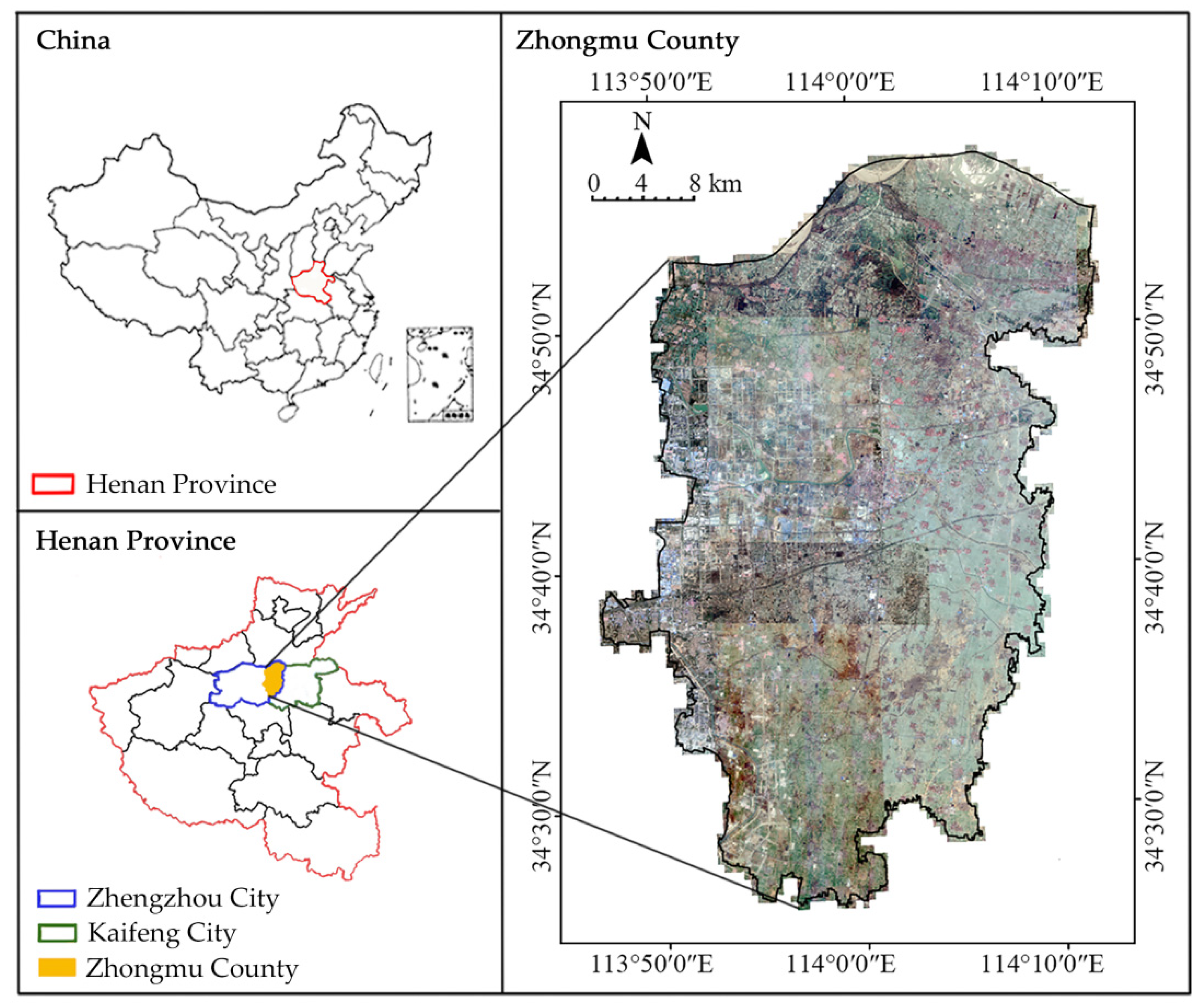
2.1. Study Area
2.2. Data Sources
2.2.1. Geospatial Data
2.2.2. Economic Data
2.3. Methods
2.3.1. Landscape Pattern Index
2.3.2. Land-Use Transfer Matrix
2.3.3. Ecosystem Service Value Assessment
2.3.4. Analysis of Cold and Hot Spots of ESV
2.3.5. Spatial Autocorrelation of ESV
3. Results
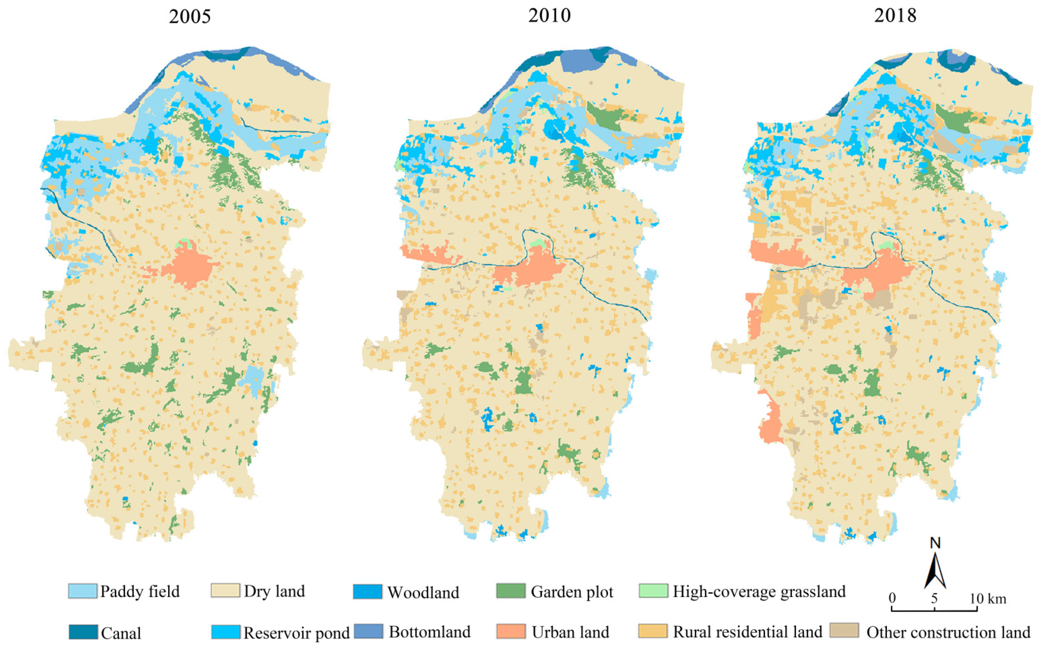
3.1. Dynamic Analysis of Landscape Pattern
3.1.1. Dynamic Analysis of the Overall Landscape
3.1.2. Analysis of Landscape Element Transfer
3.2. ESV Analysis
3.2.1. Temporal Changes in ESV
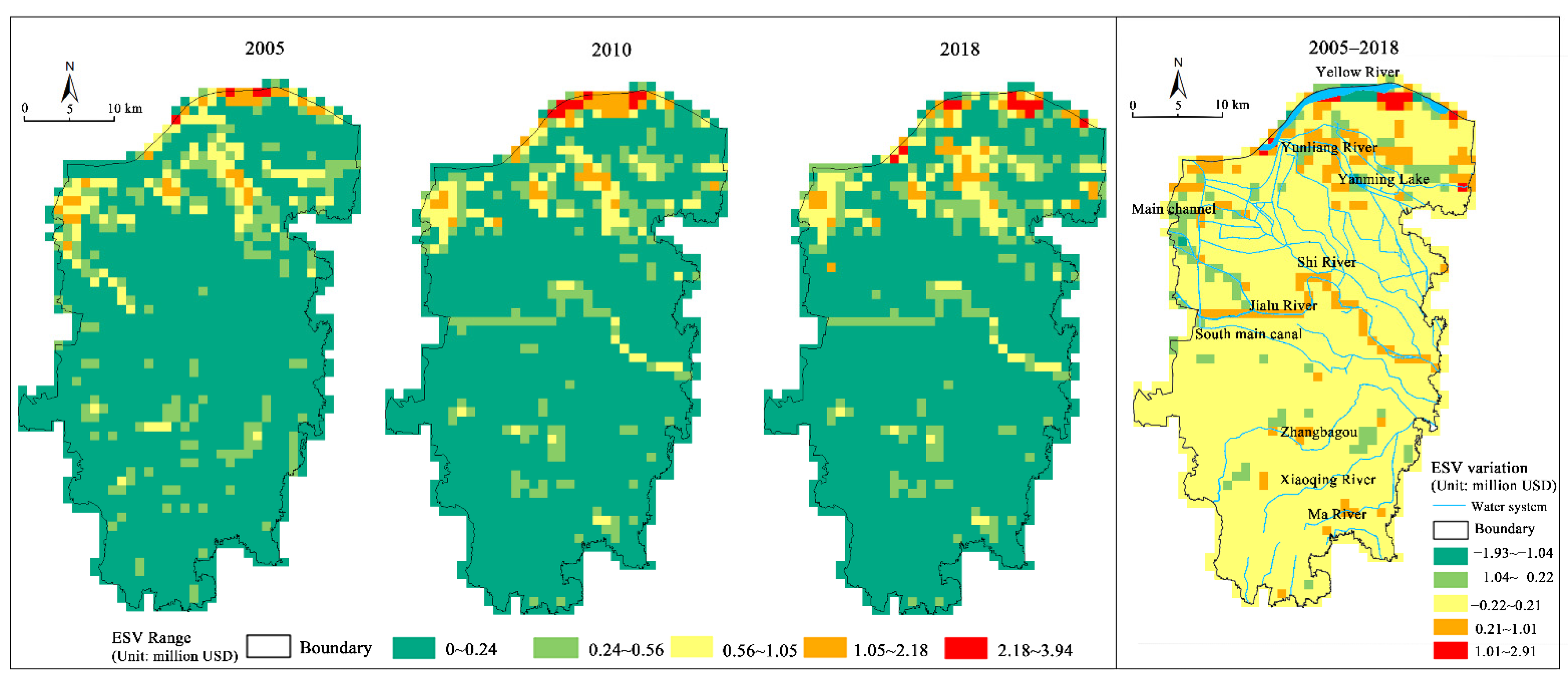
3.2.2. Spatial Changes in ESV
3.3. ESV’s Dynamic Response to Landscape Pattern
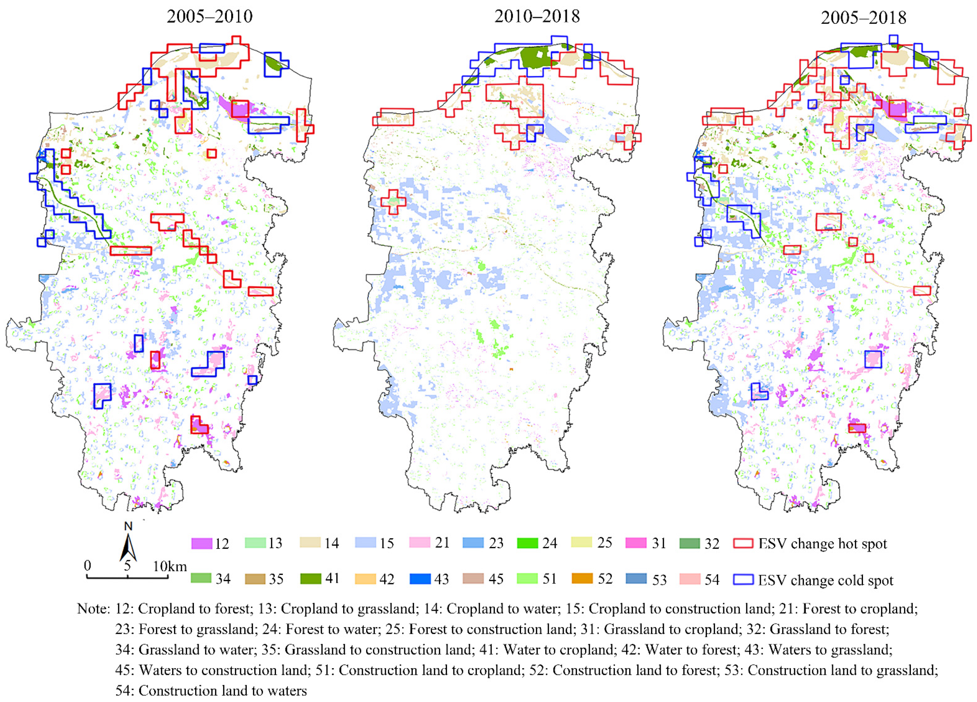
3.3.1. Landscape Transfer of ESV Changes in Cold/Hot Spots
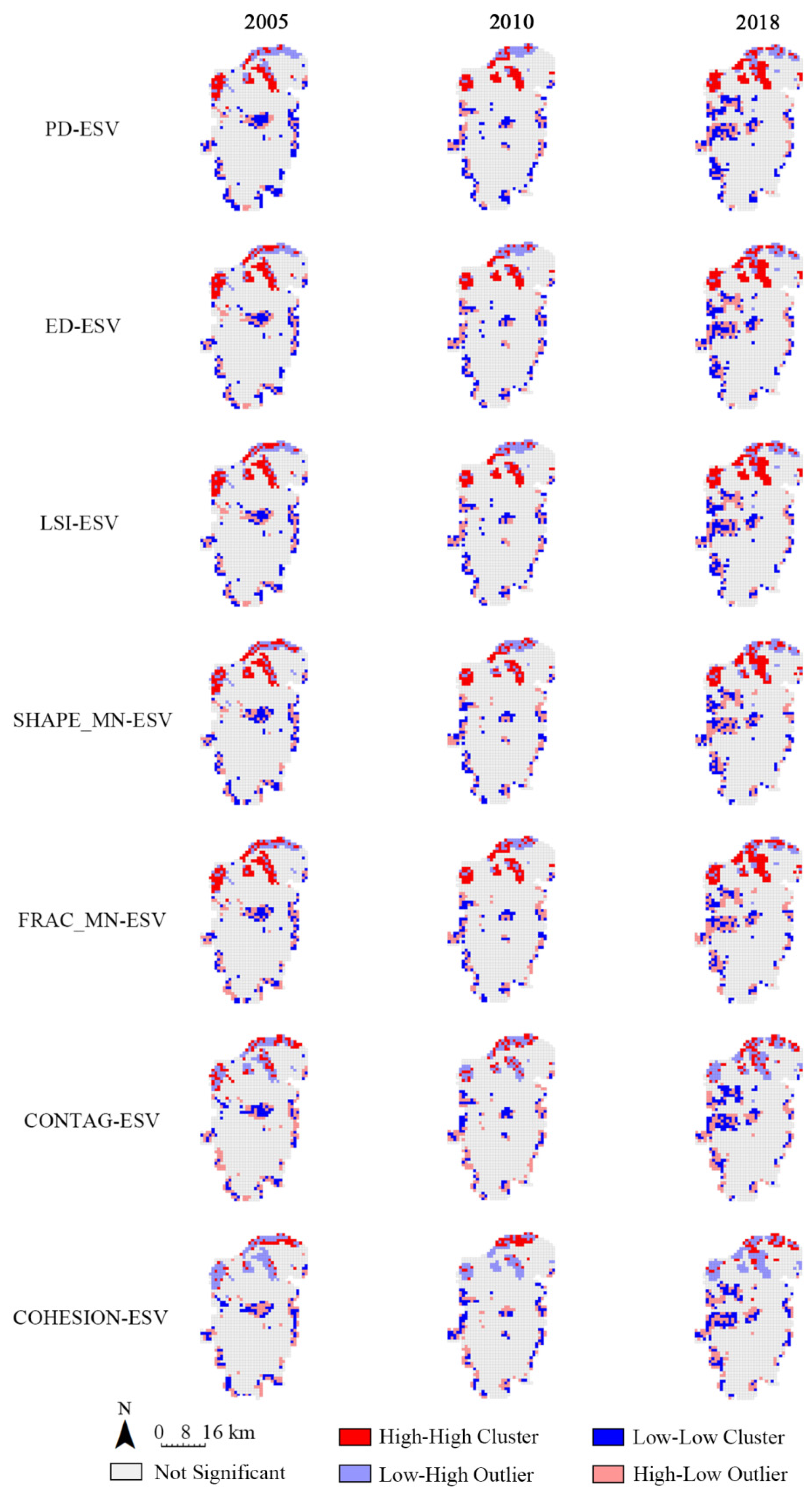
3.3.2. Spatial Correlation between ESV and Landscape-Level Index
4. Discussion
4.1. Landscape Pattern and ESV Spatio-Temporal Changes
4.1.1. Landscape Elements and ESV
4.1.2. Landscape Index and ESV
4.2. Driving Force Analysis
4.3. Optimization Measures and Outlook
- (1)
- Enhance the development the quality of green infrastructure. Improve the development level of green infrastructures such as rivers, wetlands, and woodlands to enhance the function of ecosystem services such as hydrology, climate, and soil in the region and effectively increase the total amount of ESV;
- (2)
- Control the unlimited expansion of construction land and strengthen the core ecological infrastructure. We should strictly control the unlimited expansion of construction land, optimize the layout of construction land, strengthen the intensive use, and avoid the massive erosion of arable land, water and other high-quality landscapes. At the same time, provide full play to the core advantages of the central city and strengthen the construction of “ecological green core: Zhengzhou-Kaifeng Central Park” and “ecological green core: comprehensive parks, special parks, community parks, pocket parks, etc.” Form a comprehensive park system to ensure the high quality of life for the high-density population in the central region and the stable growth of ESV;
- (3)
- Promote high-quality development of watershed ecological reserves. The Yellow River basin is the most important ecological source [49]. Further, promote the high-quality development of the ecological reserve along the Yellow River. Gradually improve the landscape pattern of the Yellow River basin with “wetland-protection forest-agricultural land”, and restore the value of the Yellow River ecosystem services.
4.4. Limitation
5. Conclusions
- (1)
- Changes in the total value of ecosystem services. The total value of ecosystem services in Zhongmu County in 2005, 2010 and 2018 showed a fluctuating trend of first increasing and then decreasing, with the total value increasing by USD 10.05 million, and the ecological environment construction achieved certain results. Spatially, the low-value area was the main area (80.01%), the high-value area was only in the local area of the Yellow River (0.53%), and the higher-value area was mainly in the Yellow River, Yanming Lake, and the paddy fields and reservoir ponds (2.36%) in the northwest corner. The spatial aggregation pattern of ecological values has a border effect: the high-high clusters area was mainly at the northern Yellow River border, while the low-low clusters area was at the east-west border, and there is an obvious trend of expansion to the east;
- (2)
- Changes in the ecosystem service values of various landscapes. The ecosystem service value of dry lands always remains the highest, with an average contribution of 37.46% to the overall value, and was the most dominant landscape in Zhongmu County in maintaining ecosystem service value, followed by reservoir ponds (14.65%) and canals (10.51%), with changes mainly related to the increase or decrease in the corresponding landscape area and value coefficients;
- (3)
- Changes in ecosystem service values of different service functions. The service functions with a higher average contribution to the ecological value of Zhongmu County were hydrological regulation (33.64%), soil conservation (12.71%) and climate regulation (10.16%), among which only the ecological value of hydrological regulation had positive growth;
- (4)
- Through the overlay analysis of the cold, hot spot and landscape transfer matrix mapping of the amount of ecosystem service change from 2005 to 2010, 2010 to 2018 and 2005 to 2018, it was found that the value of ecosystem services in the areas where cropland was transferred to waters and forests increased significantly, and the value of ecosystem services in the areas where waters were transferred to construction land and cropland decreased significantly. Therefore, we can focus on increasing watershed and forest in the landscape regulation to improve the ecosystem service value;
- (5)
- Through bivariate spatial autocorrelation analysis, it is found that the ecosystem service value can be effectively increased by enriching the landscape types and increasing the number and complexity of landscape patches in the region.
Author Contributions
Funding
Data Availability Statement
Acknowledgments
Conflicts of Interest
Appendix A

| First Classification | Secondary Classification | Description |
|---|---|---|
| Cultivated land | Paddy field | Irrigated arable land for growing rice, lotus root, and other aquatic crops, including arable land where rice and dry land crops are rotated. |
| Dry land | Cultivated land that relies on natural precipitation to grow crops and cultivated land that mainly grows vegetables. | |
| Forest | Woodland | Natural forests and artificial forests (including timber forests, economic forests, shelterbelts, etc.) with a canopy closure greater than 30%, low forest land and shrubland with a canopy closure greater than 40%, and a height of fewer than 2 m. |
| Garden plot | Unformed forest afforestation land, site, nursery and orchard, mulberry garden, tea garden, hot cropping forest garden, etc. | |
| Grassland | High-coverage grassland | Natural grassland, improved grassland and mowing grass with a coverage >50%. Generally, the water condition is good and the growth is dense. |
| Water area | Canal | Naturally formed or artificially excavated rivers and artificial canals. |
| Reservoir pond | The land below the perennial water level in the artificially constructed water storage area. | |
| Bottomland | The land between the water level of rivers and lakes during the normal period and the water level of the flood period. | |
| Construction land | Urban land | Large, medium and small cities and built-up areas above counties and towns. |
| Rural residential land | Independent of rural settlements outside of cities and towns. | |
| Other construction lands | Lands for factories and mines, large industrial areas, oil fields, saltworks, quarries, etc., as well as traffic roads, airports, and special land. |
| Landscape Pattern Index | Ecological Significance |
|---|---|
| Percentage of Landscape (PLAND) | Reflects the relative proportion of a certain landscape type to the entire landscape area [50]. |
| Largest Patch Index (LPI) | It reflects the proportion of the largest patch in the landscape area and determines the dominant type in the landscape [51]. |
| Edge Density (ED) | Reflect the degree of differentiation or fragmentation of the overall landscape patch [52]. |
| Mean Patch Fractal Dimension (FRAC_MN) | Reflect the complexity of the patch shape of the landscape type. The larger the value, the greater the space occupied by the landscape type, and the more complex its shape [53]. |
| Mean Patch Size (SHAPE_MN) | Reflects the degree of deviation of the plaque shape from the standard shape (round or square). When all patches in the landscape are square, the value is 1; when the shape of the patches deviates from the square, the value increases [54]. |
| Patch Density (PD) | Reflecting the number of patches per unit area and characterizing the complexity of landscape spatial structure, is an important indicator for evaluating landscape fragmentation [55]. |
| Patch Cohesion Index (COHESION) | Reflecting the physical connectivity of patches, the smaller the value, the more scattered the landscape patches [56,57]. |
| Landscape Shape Index (LSI) | Reflecting the overall geometric complexity of the landscape, the larger the value, the longer and irregular the boundary of the patch, the more discrete the patch, that is, the higher the complexity or fragmentation of the landscape [58]. |
| Contagion Index (CONTAG) | Reflects the degree of agglomeration or spreading trend of different plaque types. To measure to what extent landscapes are aggregated or clumped as a percentage of the maximum possible [59]. |
| Shannon’s Diversity (SHDI) | A measure of patch diversity in a landscape, which is determined by both the number of different patch types and the proportional distribution of area among patch types [60]. |
| Ecosystem Classification | Provision of Services | Supply Service | Support Service | Cultural Service | ||||||||
|---|---|---|---|---|---|---|---|---|---|---|---|---|
| First Classification | Secondary Classification | Food Production | Raw Material Production | Water Supply | Gas Regulation | Climate Regulation | Purify the Environment | Hydrological Regulation | Soil Conservation | Maintain Nutrient Circulation | Biodiversity | Aesthetic Landscape |
| Farmland | Dry land | 0.85 | 0.40 | 0.02 | 0.67 | 0.36 | 0.10 | 0.27 | 1.03 | 0.12 | 0.13 | 0.06 |
| Paddy field | 1.36 | 0.09 | −2.63 | 1.11 | 0.57 | 0.17 | 2.72 | 0.01 | 0.19 | 0.21 | 0.09 | |
| Forest | Coniferous forest | 0.22 | 0.52 | 0.27 | 1.70 | 5.07 | 1.49 | 3.34 | 2.06 | 0.16 | 1.88 | 0.82 |
| Coniferous and broad-leaved mixed | 0.31 | 0.71 | 0.37 | 2.35 | 7.03 | 1.99 | 3.51 | 2.86 | 0.22 | 2.60 | 1.14 | |
| Broadleaf | 0.29 | 0.66 | 0.34 | 2.17 | 6.50 | 1.93 | 4.74 | 2.65 | 0.20 | 2.41 | 1.06 | |
| Shrub wood | 0.19 | 0.43 | 0.22 | 1.41 | 4.23 | 1.28 | 3.35 | 1.72 | 0.13 | 1.57 | 0.69 | |
| Grassland | Grassland | 0.10 | 0.14 | 0.08 | 0.51 | 1.34 | 0.44 | 0.98 | 0.62 | 0.05 | 0.56 | 0.25 |
| Scrub-grassland | 0.38 | 0.56 | 0.31 | 1.97 | 5.21 | 1.72 | 3.82 | 2.40 | 0.18 | 2.18 | 0.96 | |
| Meadow | 0.22 | 0.33 | 0.18 | 1.14 | 3.02 | 1.00 | 2.21 | 1.39 | 0.11 | 1.27 | 0.56 | |
| Wetlands | Wetlands | 0.51 | 0.50 | 2.59 | 1.90 | 3.60 | 3.60 | 24.23 | 2.31 | 0.18 | 7.87 | 4.73 |
| Desert | Desert | 0.01 | 0.03 | 0.02 | 0.11 | 0.10 | 0.31 | 0.21 | 0.13 | 0.01 | 0.12 | 0.05 |
| Bare land | 0.00 | 0.00 | 0.00 | 0.02 | 0.00 | 0.10 | 0.03 | 0.02 | 0.00 | 0.02 | 0.01 | |
| Waters | Water system | 0.80 | 0.23 | 8.29 | 0.77 | 2.29 | 5.55 | 102.24 | 0.93 | 0.07 | 2.55 | 1.89 |
| Glacier snow | 0.00 | 0.00 | 2.16 | 0.18 | 0.54 | 0.16 | 7.13 | 0.00 | 0.00 | 0.01 | 0.09 | |
References
- Costanza, R.; d’Arge, R.; De, G.R.; Farber, S.; Grasso, M.; Hannon, B.; Limburg, K.; Naeem, S.; O’Neill, R.V.; Paruelo, J.; et al. The value of the world’s ecosystem services and natural capital. Nature 1997, 387, 253–260. [Google Scholar] [CrossRef]
- Costanza, R.; De, G.R.; Sutton, P.; Ploeg, S.; Anderson, S.J.; Kubiszewski, I.; Farber, R.S.; Turner, K. Changes in the global value of ecosystem services. Glob. Environ. Chang. 2014, 26, 152–158. [Google Scholar] [CrossRef]
- Groot, R.S.; Wilson, M.A.; Boumans, R.M.J. A typology for the classification, description and valuation of ecosystem functions, goods and services. Ecol. Economics. 2002, 41, 393–408. [Google Scholar] [CrossRef] [Green Version]
- Ojea, E.; Martin-Ortega, J.; Chiabai, A. Defining and classifying ecosystem services for economic valuation: The case of forest water services. Environ. Sci. Policy 2012, 19–20, 1–15. [Google Scholar] [CrossRef]
- Ouyang, Z.; Wang, R.; Zhao, J. Ecosystem service function and its ecological economic value evaluation. J. Appl. Ecol. 1999, 5, 635–640. [Google Scholar]
- Redford, K.H.; Adams, W.M. Payment for ecosystem services and the challenge of saving nature. Conserv. Biol. 2009, 23, 785–787. [Google Scholar] [PubMed]
- Huang, L.; Cao, W.; Xu, X.; Fan, J.; Wang, J. Linking the benefits of ecosystem services to sustainable spatial planning of ecological conservation strategies. J. Environ. Manag. 2018, 222, 385–395. [Google Scholar] [CrossRef] [PubMed]
- Li, T.; Zhang, Q.; Zhang, Y. Modelling a Compensation Standard for a Regional Forest Ecosystem: A Case Study in Yanqing District, Beijing, China. Int. J. Environ. Res. Public Health 2018, 15, 565. [Google Scholar] [CrossRef] [PubMed] [Green Version]
- Peng, J.; Yang, Y.; Liu, Y.; Hu, Y.; Du, Y. Linking ecosystem services and circuit theory to identify ecological security patterns. Sci. Total. Environ. 2018, 644, 787–790. [Google Scholar] [CrossRef] [Green Version]
- Shi, P.; Zhang, X.; Luo, J.; Zhang, X. Response of Ecological Services Value to Land Use Change in the Shiyang River Basin: A Case Study in Wuwei Region. Adv. Mater. Res. 2012, 518–523, 5116–5120. [Google Scholar] [CrossRef]
- Su, C.; Fu, B. The relationship between landscape pattern and ecological process and its impact on ecosystem services. J. Nat. 2012, 34, 277. [Google Scholar]
- Renetzeder, C.; Schindler, S.; Peterseil, J.; Prinz, M.A.; Mücher, S.; Wrbka, T. Can we measure ecological sustainability? Landscape pattern as an indicator for naturalness and land use intensity at regional, national and European level. Ecol. Indic. 2009, 10, 39–48. [Google Scholar] [CrossRef]
- Hof, J.; Flather, C. Key Topics In Landscape Ecology: Optimization Of Landscape Pattern; Cambridge University Press: Cambridge, UK, 2007; pp. 39–61. [Google Scholar]
- Li, L.; Wu, D.; Liu, Y. Research hotspots and trends of land use and ecosystem services at home and abroad—Based on CiteSpace measurement analysis. Res. Soil Water Conserv. 2020, 27, 396–404. [Google Scholar]
- Shen, G.; Yang, X.; Jin, Y.; Luo, S.; Zhou, Q. Land Use Changes in the Zoige Plateau Based on the Object-Oriented Method and Their Effects on Landscape Patterns. Remote. Sens. 2019, 12, 14. [Google Scholar] [CrossRef] [Green Version]
- Nelson, E.; Mendoza, G.; Regetz, J.; Polasky, S.; Tallis, H.; Cameron, D.R.; Chan, K.M.A.; Daily, G.C.; Goldstein, J.; Kareiva, P.M.; et al. Modeling Multiple Ecosystem Services, Biodiversity Conservation, Commodity Production, and Tradeoffs at Landscape Scales. Front. Ecol. Environ. 2009, 7, 4–11. [Google Scholar] [CrossRef]
- Grêt-Regamey, A.; Rabe, S.E.; Crespo, R.; Crespo, R.; Lautenbach, S.; Ryffel, A.; Schlup, B. On the importance of non-linear relationships between landscape patterns and the sustainable provision of ecosystem services. Landsc. Ecol. 2014, 29, 201–212. [Google Scholar] [CrossRef]
- Soy-Massoni, E.; Langemeyer, J.; Varga, D.; Sáez, M.; Pintó, J. The importance of ecosystem services in coastal agricultural landscapes: Case study from the Costa Brava, Catalonia. Ecosyst. Serv. 2016, 17, 43–52. [Google Scholar] [CrossRef]
- Cen, X. Association Analysis and Optimization of Land Use Landscape Pattern and Ecosystem Service Value; Zhejiang University: Hangzhou, China, 2016. [Google Scholar]
- Guo, M.; Shu, S.; Ma, S.; Wang, L. Using high-resolution remote sensing images to explore the spatial relationship between landscape patterns and ecosystem service values in regions of urbanization. Environ. Sci. Pollut. Res. 2021, 1–3. [Google Scholar] [CrossRef]
- Feng, Y.; Zhu, J.; Zeng, L.; Xiao, W. Ecosystem service value profit and loss prediction under county land use changes: A case study in Banan District, Chongqing City. Chin. J. Ecol. Sci. 2021, 9, 1–13. [Google Scholar]
- National Bureau of Statistics. Available online: http://www.stats.gov.cn/tjsj/ndsj/ (accessed on 14 August 2021).
- Xia, H.; Ge, S.; Zhang, X.; Lei, Y.; Liu, Y. Spatiotemporal Dynamics of Green Infrastructure in an Agricultural Peri-Urban Area: A Case Study of Baisha District in Zhengzhou, China. Land 2021, 10, 801. [Google Scholar] [CrossRef]
- Lei, Y. Deepen the research on the integration of Zhengzhou and Kaifeng under the background of Zhengzhou central city construction. Times Econ. Trade 2018, 18, 18–19. [Google Scholar]
- Cui, Y.; Li, G. Research on the in-depth promotion of Zhengzhou and Kaifeng integration. J. Hubei Univ. Econ. Humanit. Soc. Sci. Ed. 2013, 10, 24–25. [Google Scholar]
- Zhongmu County People’s Government. Available online: http://www.zhongmu.gov.cn/sitesources/zmxzf/page_pc/zwgk/tzgg/articlef9acda8975ee49efb5f5a8740fa56688.html (accessed on 8 June 2016).
- Yinkfu, N.N.; Mbue, I.N. Estimation for Groundwater Balance Based on Recharge and Discharge: A Tool for Sustainable Groundwater Management, Zhongmu County Alluvial Plain Aquifer, Henan Province, China. J. Am. Sci. 2009, 5, 83–90. [Google Scholar]
- Nan, J.; Xiao, X. Analysis of Land Use in Jining City. E3S Web of Conferences. EDP Sci. 2020, 198, 04024. [Google Scholar]
- Lv, C.; Wang, J.; Li, Y.; He, T. Land use change and its effects on eco-environment in Bashang area of Hebei province. SPIE Remote. Sens. 2005, 5983, 59830J. [Google Scholar]
- Xie, G.; Lu, C.; Leng, Y.; Zheng, D.; Li, S. Value evaluation of ecological assets in the Qinghai-Tibet Plateau. J. Nat. Resour. 2003, 18, 189–195. [Google Scholar]
- Xie, G.; Zhang, C.; Zhang, C.; Xiao, Y.; Lu, C. The value of ecosystem services in China. Resour. Sc. 2015, 37, 1740–1746. [Google Scholar]
- Duan, Y.; Lei, Y.; Ma, G.; Wu, B.; Tian, G. Temporal and spatial changes of ecosystem service value in Zhengzhou City. J. Zhejiang AF Univ. 2017, 34, 511–519. [Google Scholar]
- Zhang, Q.; Gao, M.; Yang, L.; Cheng, C.; Sun, Y.; Wang, J. Spatial structure of ecological land and changes in ecosystem service value in the nine districts of the main city of Chongqing from 1988 to 2013. Acta Ecol. Sin. 2017, 37, 566–575. [Google Scholar]
- Hu, M.; Li, T.; Wang, F.; Jiao, M.; Li, M.; Xia, B. Spatio-temporal changes in ecosystem service value in response to land-use/cover changes in the Pearl River Delta. Resour. Conserv. Recycl. 2019, 149, 106–114. [Google Scholar] [CrossRef]
- Dormann, C.F.; Mcpherson, J.M.; Araújo, M.B.; Bivand, R.; Bolliger, J.; Carl, G.; Davies, R.G.; Hirzel, A.; Jetz, W.; Kissling, W.D. Methods to account for spatial autocorrelation in the analysis of species distributional data: A review. Ecography 2007, 30, 609–628. [Google Scholar] [CrossRef] [Green Version]
- Zhang, J.Q.; Gu, J.; Ma, X.C.; Liu, D.-Q. GeoDA-based spatial correlation analysis of landscape fragmentation in Bailongjiang Watershed of Gansu. Chin. J. Ecol. 2018, 37, 1476–1483. [Google Scholar]
- Xie, H.; Kung, C.-C.; Zhao, Y. Spatial disparities of regional forest land change based on ESDA and GIS at the county level in Beijing-Tianjin-Hebei area. Front. Earth Sci. 2012, 6, 445–452. [Google Scholar] [CrossRef]
- Zhao, H.; Duan, X.; Stewart, B.; You, B.; Jiang, X. Spatial correlations between urbanization and river water pollution in the heavily polluted area of Taihu Lake Basin, China. J. Geogr. Sci. 2013, 23, 735–752. [Google Scholar] [CrossRef]
- Hou, L.; Wu, F.; Xie, X. The spatial characteristics and relationships between landscape pattern and ecosystem service value along an urban-rural gradient in Xi’an city, China. Ecol. Indic. 2020, 108, 105720. [Google Scholar] [CrossRef]
- Assefa, W.W.; Eneyew, B.G.; Wondie, A. The impacts of land-use and land-cover change on wetland ecosystem service values in peri-urban and urban area of Bahir Dar City, Upper Blue Nile Basin, Northwestern Ethiopia. Ecol. Process. 2021, 10, 1–18. [Google Scholar] [CrossRef]
- Lin, M.; Zhou, R.; Zhong, L. Research on changes in ecosystem services in the Guangdong-Hong Kong-Macao Greater Bay Area based on changes in landscape pattern. J. Guangzhou Univ. Nat. Sci. Ed. 2019, 18, 87–95. [Google Scholar]
- Gu, Z.; Zhao, X.; Gao, X.; Xie, P. Landscape pattern change and evaluation of ecosystem service value in Lancang County. Ecol. Sci. 2016, 35, 143–153. [Google Scholar]
- Qiu, L.; Pan, Y.; Zhu, J.; Amable, G.S.; Xu, B. Integrated analysis of urbanization-triggered land use change trajectory and implications for ecological land management: A case study in Fuyang, China. Sci. Total Environ. 2019, 660, 209–217. [Google Scholar] [CrossRef]
- Raviv, O.; Shamir, S.Z.; Izhaki, I.; Alon, L. The effect of wildfire and land-cover changes on the economic value of ecosystem services in Mount Carmel Biosphere Reserve, Israel. Ecosyst. Serv. 2021, 49, 101291. [Google Scholar] [CrossRef]
- Mendoza-González, G.; Martínez, M.L.; Lithgow, D.; Pérez-Maqueo, O.; Simonin, P. Land use change and its effects on the value of ecosystem services along the coast of the Gulf of Mexico. Ecol. Econ. 2012, 82, 23–32. [Google Scholar] [CrossRef]
- Li, H. Research on accelerating the construction of the Greater Zhengzhou Metropolitan Area and promoting the integrated development of the metropolitan area and surrounding cities. Beauty Times Urban Ed. 2017, 11, 1–2. [Google Scholar]
- The People’s Government of Henan Province. Available online: https://www.henan.gov.cn/2007/03-05/270848.html (accessed on 5 March 2007).
- The People’s Government of Henan Province. Available online: https://www.henan.gov.cn/2007/02-01/245501.html (accessed on 1 February 2007).
- Yang, J.; Xie, B.; Zhang, D.; Tao, W. Climate and land use change impacts on water yield ecosystem service in the Yellow River Basin, China. Environ. Earth Sci. 2021, 80, 72. [Google Scholar] [CrossRef]
- Nita, M.R.; Nastase, I.I.; Badiu D, L.; Gavrilidis, A.A. Evaluating urban forests connectivity in relation to urban functions in romanian cities. Carpathian J. Earth Environ. Sci. 2018, 13, 291–299. [Google Scholar] [CrossRef]
- Zhang, Q.; Chen, C.; Wang, J.; Yang, D.; Zhang, Y.; Wang, Z.; Gao, M. The spatial granularity effect, changing landscape patterns, and suitable landscape metrics in the Three Gorges Reservoir Area, 1995–2015. Ecol. Indic. 2020, 114, 15. [Google Scholar] [CrossRef]
- Zhang, D.; Wang, W.; Zheng, H.; Ren, Z.; Zhai, C.; Tang, Z.; Shen, G.; He, X. Effects of urbanization intensity on forest structural-taxonomic attributes, landscape patterns and their associations in Changchun, Northeast China: Implications for urban green infrastructure planning. Ecol. Indic. 2017, 80, 286–296. [Google Scholar] [CrossRef]
- Ouyang, W.; Skidmore, A.K.; Hao, F.; Toxopeus, A.G.; Abkar, A. Accumulated effects on landscape pattern by hydroelectric cascade exploitation in the Yellow River basin from 1977 to 2006. Landsc. Urban Plan. 2009, 93, 163–171. [Google Scholar] [CrossRef]
- Byomkesh, T.; Nakagoshi, N.; Dewan, A.M. Urbanization and green space dynamics in Greater Dhaka, Bangladesh. Landsc. Ecol. Eng. 2012, 8, 45–58. [Google Scholar] [CrossRef]
- Lamine, S.; Petropoulos, G.P.; Singh, S.K.; Szabó, S.; Bachari, N.E.Y.; Srivastava, P.K.; Suman, S. Quantifying land use/land cover spatio-temporal landscape pattern dynamics from Hyperion using SVMs classifier and FRAGSTATS((R)). Geocarto Int. 2018, 33, 862–878. [Google Scholar] [CrossRef]
- Zhang, L.; Hou, G.; Li, F. Dynamics of landscape pattern and connectivity of wetlands in western Jilin Province, China. Environ. Dev. Sustain. 2020, 22, 2517–2528. [Google Scholar] [CrossRef]
- Plexida, S.G.; Sfougaris, A.I.; Ispikoudis, I.P.; Papanastasis, V.P. Selecting landscape metrics as indicators of spatial heterogeneity-A comparison among Greek landscapes. Int. J. Appl. Earth Obs. Geoinf. 2014, 26, 26–35. [Google Scholar] [CrossRef]
- Dong, J.; Dai, W.; Shao, G.; Xu, J. Ecological Network Construction Based on Minimum Cumulative Resistance for the City of Nanjing, China. Isprs Int. J. Geoinf. 2015, 4, 2045–2060. [Google Scholar] [CrossRef] [Green Version]
- Chen, L.; Wang, Q. Spatio-temporal evolution and influencing factors of land use in Tibetan region: 1995–2025. Earth Sci. Inform. 2021, 1–12. [Google Scholar] [CrossRef]
- Zhang, L.; Wu, J.; Yu, Z.; Shu, J. RETRACTED: A GIS-based gradient analysis of urban landscape pattern of Shanghai metropolitan area, China. Landsc. Urban Plan. 2004, 69, 1–16. [Google Scholar] [CrossRef]

| Scatter Image Limit | LISA Gathering | Spatial Correlation | Description |
|---|---|---|---|
| First quadrant | High-High Cluster | Positive spatial correlation | The element values of the spatial unit and its forest are high, and the spatial difference is small. |
| Second quadrant | Low-High Outlier | Spatial negative correlation | The element value of the spatial unit is low, the element value of its neighborhood is high, and the spatial difference is large. |
| Third quadrant | Low-Low Cluster | Positive spatial correlation | The feature value of the spatial unit and its neighborhood is low, and the spatial difference is small. |
| Fourth quadrant | High-Low Outlier | Spatial negative correlation | The higher the element value of a spatial unit, the lower the element value of its neighbors, and the greater the spatial difference. |
| Years | ED | FRAC_MN | SHAPE_MN | PD | COHESION | LSI | CONTAG | SHDI |
|---|---|---|---|---|---|---|---|---|
| 2005 | 10.13 | 1.06 | 1.50 | 0.31 | 99.86 | 14.95 | 74.56 | 1.18 |
| 2010 | 10.58 | 1.07 | 1.55 | 0.32 | 99.87 | 15.57 | 73.82 | 1.21 |
| 2018 | 11.40 | 1.07 | 1.56 | 0.34 | 99.79 | 16.70 | 72.35 | 1.28 |
| 2018 | Paddy Field | Dry Land | Woodland | Garden Plot | High-Coverage Grassland | Canal | Reservoir Pond | Bottomland | Urban Land | Rural Residential Land | Other Construction Lands | Reduction | |
|---|---|---|---|---|---|---|---|---|---|---|---|---|---|
| 2005 | |||||||||||||
| Paddy field | 44.55 | 42.06 | 0.00 | 0.02 | 1.05 | 0.02 | 13.51 | 0.00 | 4.53 | 7.44 | 6.57 | 75.20 | |
| Dry land | 25.10 | 785.48 | 6.13 | 18.60 | 1.78 | 8.75 | 13.57 | 2.14 | 24.16 | 73.80 | 32.77 | 206.80 | |
| Woodland | 0.30 | 0.33 | 0.00 | 0.00 | 0.00 | 0.00 | 0.00 | 0.00 | 0.00 | 0.00 | 0.00 | 0.63 | |
| Garden plot | 0.60 | 30.14 | 2.33 | 19.27 | 0.21 | 0.08 | 2.39 | 0.00 | 0.90 | 2.53 | 1.72 | 40.89 | |
| High-coverage grassland | 0.00 | 0.21 | 0.00 | 0.00 | 0.79 | 0.00 | 0.00 | 0.00 | 0.02 | 0.00 | 0.07 | 0.30 | |
| Canal | 0.33 | 4.65 | 0.00 | 0.46 | 0.05 | 1.17 | 1.39 | 0.55 | 0.18 | 0.03 | 0.05 | 7.68 | |
| Reservoir pond | 3.51 | 4.44 | 0.01 | 0.25 | 0.90 | 0.00 | 26.86 | 0.00 | 0.00 | 2.50 | 4.50 | 16.11 | |
| Bottomland | 0.00 | 7.43 | 0.00 | 0.00 | 0.23 | 3.94 | 0.41 | 3.76 | 0.00 | 0.47 | 0.00 | 12.47 | |
| Urban land | 0.00 | 3.25 | 0.00 | 0.00 | 0.42 | 0.16 | 0.00 | 0.00 | 15.92 | 1.02 | 0.27 | 5.12 | |
| Rural residential land | 1.11 | 27.01 | 0.19 | 0.86 | 0.07 | 0.08 | 1.15 | 0.00 | 5.82 | 71.38 | 2.41 | 38.69 | |
| Other construction land | 0.28 | 3.05 | 0.00 | 0.34 | 0.00 | 0.02 | 0.09 | 0.00 | 0.85 | 1.21 | 0.61 | 5.83 | |
| Increments | 31.22 | 122.56 | 8.67 | 20.52 | 4.69 | 13.04 | 32.51 | 2.68 | 36.47 | 89.02 | 48.35 | - | |
| 2005 | 2010 | 2018 | 2005–2018 | |||
|---|---|---|---|---|---|---|
| Landscape Type | ESV/USD Million | ESV/USD Million | ESV/USD Million | Change Value/USD Million | Rate of Change/% | Average Contribution Rate/% |
| Dry land | 129.06 | 128.18 | 118.10 | −10.96 | −8.49 | 37.46 |
| Paddy field | 15.11 | 10.17 | 9.56 | −5.55 | −36.73 | 3.49 |
| Woodland | 0.47 | 6.85 | 6.49 | 6.01 | 1267.46 | 1.36 |
| Garden plot | 45.06 | 30.07 | 29.80 | −15.26 | −33.86 | 10.51 |
| High-coverage grassland | 0.69 | 3.52 | 3.50 | 2.81 | 404.56 | 0.76 |
| Reservoir pond | 72.49 | 76.93 | 100.17 | 27.68 | 38.18 | 24.88 |
| Bottomland | 27.39 | 30.80 | 10.87 | −16.52 | −60.32 | 6.90 |
| Canal | 36.04 | 53.38 | 57.87 | 21.82 | 60.55 | 14.65 |
| Total | 326.32 | 339.90 | 336.36 | 10.05 | 3.08 | 100.00 |
| Level 1 Function | Secondary Function | Rate of Change/% | Average Contribution Rate/% | ||
|---|---|---|---|---|---|
| 2005–2010 | 2010–2018 | 2005–2018 | |||
| Provision of services | Food production | −5.18 | −7.03 | −11.85 | 9.74 |
| Raw material production | −1.78 | −6.49 | −8.16 | 4.54 | |
| Water supply | −323.12 | 24.53 | −377.84 | 0.58 | |
| Regulation service | Gas regulation | −5.10 | −5.43 | −10.25 | 9.79 |
| Climate regulation | −5.14 | −2.62 | −7.62 | 10.16 | |
| Purify the environment | 3.52 | 0.55 | 4.09 | 5.02 | |
| Hydrological regulation | 13.21 | 3.45 | 17.11 | 33.64 | |
| Support service | Soil conservation | −1.11 | −5.78 | −6.82 | 12.71 |
| Maintain nutrient circulation | −5.31 | −6.32 | −11.29 | 1.53 | |
| Biodiversity | 2.26 | 0.60 | 2.87 | 7.93 | |
| Cultural service | Aesthetic landscape | 3.95 | 1.16 | 5.16 | 4.37 |
| Total | 4.16 | −1.04 | 3.08 | 100.00 | |
| ESV Range (Unit: USD million) | Grade | 2005 | 2010 | 2018 | Average Percentage/% |
|---|---|---|---|---|---|
| Quantity | Quantity | Quantity | |||
| 0–0.24 | Low-value area | 1213 | 1217 | 1197 | 80.01 |
| 0.24–0.56 | Lower-value area | 170 | 161 | 169 | 11.03 |
| 0.56–1.05 | Median zone | 94 | 86 | 95 | 6.07 |
| 1.05–2.18 | Higher-value area | 30 | 38 | 39 | 2.36 |
| 2.18–3.94 | High-value area | 4 | 9 | 11 | 0.53 |
| Total | 1511 | 1511 | 1511 | 100 | |
| Landscape Level Index | 2005 | 2010 | 2018 |
|---|---|---|---|
| PD | 0.120 | 0.101 | 0.140 |
| ED | 0.118 | 0.080 | 0.135 |
| LSI | 0.118 | 0.080 | 0.135 |
| SHAPE_MN | 0.067 | 0.027 | 0.061 |
| FRAC_MN | 0.083 | 0.039 | 0.050 |
| CONTAG | −0.021 | −0.002 | −0.019 |
| COHESION | −0.181 | −0.123 | −0.054 |
Publisher’s Note: MDPI stays neutral with regard to jurisdictional claims in published maps and institutional affiliations. |
© 2021 by the authors. Licensee MDPI, Basel, Switzerland. This article is an open access article distributed under the terms and conditions of the Creative Commons Attribution (CC BY) license (https://creativecommons.org/licenses/by/4.0/).
Share and Cite
Zhang, X.; Li, H.; Xia, H.; Tian, G.; Yin, Y.; Lei, Y.; Kim, G. The Ecosystem Services Value Change and Its Driving Forces Responding to Spatio-Temporal Process of Landscape Pattern in the Co-Urbanized Area. Land 2021, 10, 1043. https://doi.org/10.3390/land10101043
Zhang X, Li H, Xia H, Tian G, Yin Y, Lei Y, Kim G. The Ecosystem Services Value Change and Its Driving Forces Responding to Spatio-Temporal Process of Landscape Pattern in the Co-Urbanized Area. Land. 2021; 10(10):1043. https://doi.org/10.3390/land10101043
Chicago/Turabian StyleZhang, Xinyu, Huawei Li, Hua Xia, Guohang Tian, Yuxing Yin, Yakai Lei, and Gunwoo Kim. 2021. "The Ecosystem Services Value Change and Its Driving Forces Responding to Spatio-Temporal Process of Landscape Pattern in the Co-Urbanized Area" Land 10, no. 10: 1043. https://doi.org/10.3390/land10101043
APA StyleZhang, X., Li, H., Xia, H., Tian, G., Yin, Y., Lei, Y., & Kim, G. (2021). The Ecosystem Services Value Change and Its Driving Forces Responding to Spatio-Temporal Process of Landscape Pattern in the Co-Urbanized Area. Land, 10(10), 1043. https://doi.org/10.3390/land10101043