Combining Remote Sensing and Species Distribution Modelling to Assess Pinus hartwegii Response to Climate Change and Land Use from Izta-Popo National Park, Mexico

Abstract

A detailed analysis of distribution shifts in Pinus hartwegii Lindl. is provided across time for Izta-Popo National Park (México). Combining satellite images, species distribution models, and connectivity analysis we disentangled the effect of climate change and anthropogenic land use on the habitat availability. Twenty-four Maxent habitat suitability models with varying complexity were combined with insights on vegetation and land cover change derived from two Landsat satellite images at 30-m resolution from 1993 and 2013. To evaluate effects of climate change on Izta-Popo’s P. hartwegii forest, projections for future climatic conditions (averaged for 2050 and 2070) were derived using two General Circulation Models under three Representative CO₂ concentration pathways (RCPs). Calculated fragmentation and connectivity indexes (Equivalent Connected Area and Probability of Connectivity metrics) showed significant habitat loss and habitat fragmentation that weakens P. hartwegii dispersion flux and the strength of connections. Projections of future climate conditions showed a reduction of P. hartwegii habitat suitability as populations would have to migrate to higher altitudes. However, the impact of anthropogenic land use change documented over the 20 years masks the predicted impact of climate change in Izta-Popo National Park.

1. Introduction

Studies over the last three decades have shown that land change and climate changes produce major impacts on biological systems across many scales [1]. The work by Foden et al. [2] provides an overview of this exponentially developing field of climate change vulnerability assessment of species to choose effective conservation strategies. However, there is an ongoing challenge to reduce uncertainties on the quantification of climate change and land use impacts, particularly in heterogeneous areas or those more intensively affected, typified in mountain ecosystems [3,4]. Usually, in these areas, species’ inventories are incomplete and climate models are inaccurate due to the lack of meteorological stations at high altitudes [5]. Here, the combination of the widely accessible remote sensing data with field-based climate change impact models can be used as an alternative approach to improve land use and climate change vulnerability assessment of ecosystems.

Species Distribution Models (SDM) can be used to forecast climate change impacts on species’ distributions [6,7,8]. SDM are based on modeling the potential distribution of a species by establishing algorithms between (1) field observation points as a current species distribution proxy, and (2) their current associated environmental conditions as predictor variables [9,10]. This correlative approach, often conducted at a 1-km² scale, considers climate as the dominant environmental factor defining the “fundamental ecological niche” of a species’ distribution [11]. Such correlations can be projected to future climate conditions associated with different anthropogenic scenarios, to evaluate habitat suitability impacts. This approach is strongly dependent on the different algorithms used, the selection of predictor variables, and the quantity and quality of the input data used to construct the models [12,13,14,15]. Maxent, the modeling technique employed here, uses the principle of maximum entropy on presence-only data to estimate the relative suitability of habitat in the study area [16,17]; this can overfit the training data, making transferability unreliable [18]. To control overfitting, parallel to choices on function settings and the number of explaining variables, Maxent uses a β regularization parameter that relaxes the suitability functions to lie within an interval around the empirical mean rather than matching it exactly [17]. The pre-selected features, explaining variables and β-parameter, define the complexity level of each Maxent model as quoted on the “number of parameters” [16].

To compare the different model selections, their predictive ability must be evaluated, ideally with independent observations [19]. However, due to the lack of such data, validation is performed by dividing the presence data set into a ‘calibration’ and a ‘validation’ data set [20].

Biased or incomplete field data are common due to environmental, economic, or security handicaps (as in this case study), where data are not collected across the environmental range, in more inaccessible areas, or from conflict zones, respectively. These issues combine to result in an incomplete picture of the realized niche [11,21]. Using alternative sources of presence data would benefit the calibration and validation modeling processes, especially in remote areas that house an important part of the world biodiversity. Here, Remote Sensing Data (RSD) stands out as an alternative low-cost and independent data to cross-validate SDM, while furthermore informing about habitat structure changes through time at a complementary spatio-temporal scale, accounting for biological interactions and human activity [9,11].

Satellite spectral information (RSD) in combination with attributes obtained from inventory plots is a growing research field to investigate ecosystem functioning and to detect plant assemblages or ecosystem properties’ changes in time that complement in situ terrestrial monitoring approaches [22,23]. Multi-spectral biophysical estimates of vegetation have been used to map large areas of forests [24] or to assist forest surveys for stratification and post-stratification field sampling [25]. The continuous advances on multi- and hyper-spectral approaches and techniques to obtain biophysical estimates at higher temporal and spatial resolution [26,27,28] in parallel increasing quality and accessibility of in situ observations [29] open new horizons in biodiversity studies [30]. However, few studies integrate RSD with SDM, and usually they are limited to the inclusion of RSD estimates as explanatory variables to calibrate SDM; this handicaps the possibility to project such models under future scenarios due to the absence of RSD estimates in future conditions [31,32,33].

In areas where a lack of data field information exists, RSD have been proven to provide valuable and complementary information in landscape structure (i.e., disruption of the landscape patters, resulting in habitat loss, habitat fragmentation, and connectivity) at broad scales [34,35,36,37,38,39]. Importantly, habitat loss and fragmentation due to anthropogenic land use change is a major ecological concern that might result in a decrease of habitat availability and reachability (i.e., the amount of habitat and capacity to move among habitat patches) that can lead to habitat isolation, decrease of genetic diversity, and population decline or local extinctions [40,41,42].

Connectivity analyses have shown a great utility and effectiveness to guide conservation efforts to preserve and restore habitat connectivity in a cost-effective way, e.g., [43,44]. These studies normally focus on characterizing ecological networks in order to quantify functional habitat changes along time and providing explicit information about the most important areas for genes and species to move [43,45]. Recently, some studies have highlighted the contribution of RSD to derive more accurate connectivity predictions with a large potential to support the best-informed conservation plans, e.g., [40,42].

In this work, we show a framework for habitat evaluation across time to overcome limitations of field-based data by integrating RSD, correlative distribution models, and connectivity metrics. First, the climate change effect on Pinus hartwegii Lindl. habitat suitability was tracked by the projections of Maxent models to future climate conditions on Izta Popo National Park. Second, the variation of P. hartwegii habitat distribution and its connectivity observed on the land cover variation during a 20-year interval (tracked by RSD) were investigated. Our results help a spatially explicit understanding of P. hartwegii distribution under climate change, giving support to develop management recommendations for its conservation.

2. Materials and Methods

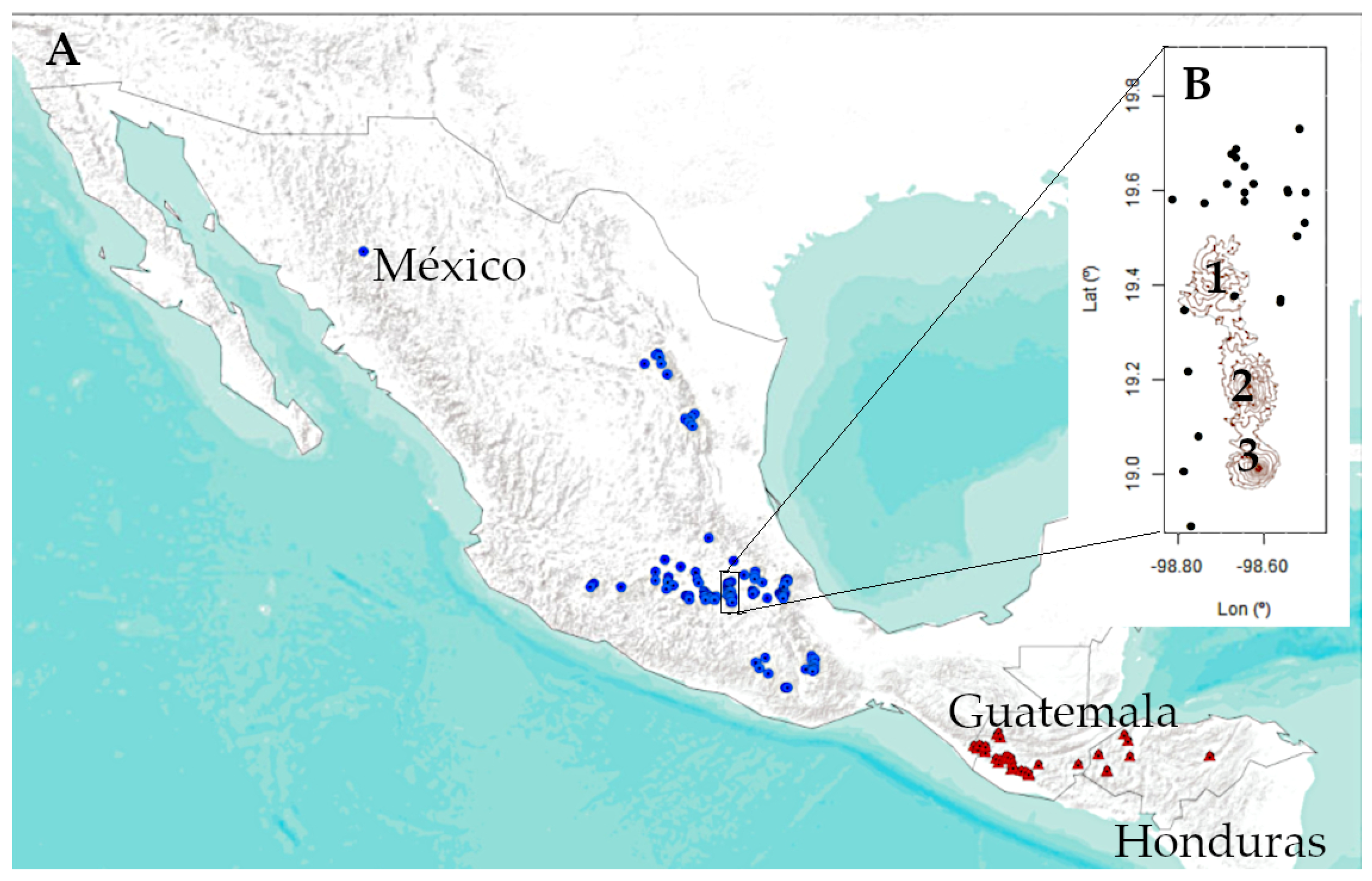
2.1. Species and Study Area

The re-sprouting 30-m-tall P. hartwegii is found naturally in Mexico, Guatemala, and Honduras mountain summits, between 2300 to 4300 m above sea level (m a.s.l.) [46,47] (Figure 1), making it an ideal candidate to explore modeling challenges on mountain areas. The main range of the species is found in México, where P. hartwegii dominates forest up to the tree line ~4000 m a.s.l., forming pure stands above 3000 m a.s.l. [48]. At present, the 1:125,00 INEGI vegetation map only provides for rough limits’ distribution of the p. hartwegii target species [49]. Species’ occurrence information can be found from the Mexican Forest Inventory [48,50] and from the Atlas of the world’s conifers [47].

Ranging from 3600 to 5480 m a.s.l., and covering an area of 39,819.09 ha, the Izta-Popo National Park hosts two of the three highest volcanoes in Mexico (Figure 1). This area provides for key environmental services (e.g., water, timber, carbon storage) to Morelos, Puebla, and downstream Mexican states. The climate is characterized by 928 mm mean annual rainfall, with September being the wettest month (185.6 mm) and February the driest (6.9 mm). The monthly mean temperature is 14.5 ± 5.4 °C. January with 10.8 °C and May with 16.2 °C are the coldest and warmest months, respectively [48].

Following Rzedowski’s classification of the Mexican vegetation in 1978, three vegetation zones have been distinguished in Izta-Popo National Park; these are strongly dependent on the altitude and orientation [48]. On the most hygrophilic areas of the basal belt (below ~3700 m a.s.l.), a Pino-Oyamel (i.e., Pinus hartwegii Lindl.—Abies religiosa Kunth Schltdl. et Cham.) mixed forest can be found. Pinus ayacahuite Ehrenb. ex Schltdl. and P. montezumae Lamb. are found on more xerophytic areas, up to this ~3400 m a.s.l. Above this altitude a second vegetation zone is formed by P. hartwegii monospecific forests alternating with altitudinal pastures that dominate above ~4000 m a.s.l. (third vegetation zone). From ~4500 m a.s.l., glaciers inhibit the establishment of permanent vegetation. More vegetation types can be found in the areas surrounding Izta-Popo National Park, below 3600 m a.s.l., where Pinus montezumae-Stipa spp. or Pinus leiophylla-Stellaria cuspidate associations grow [52].

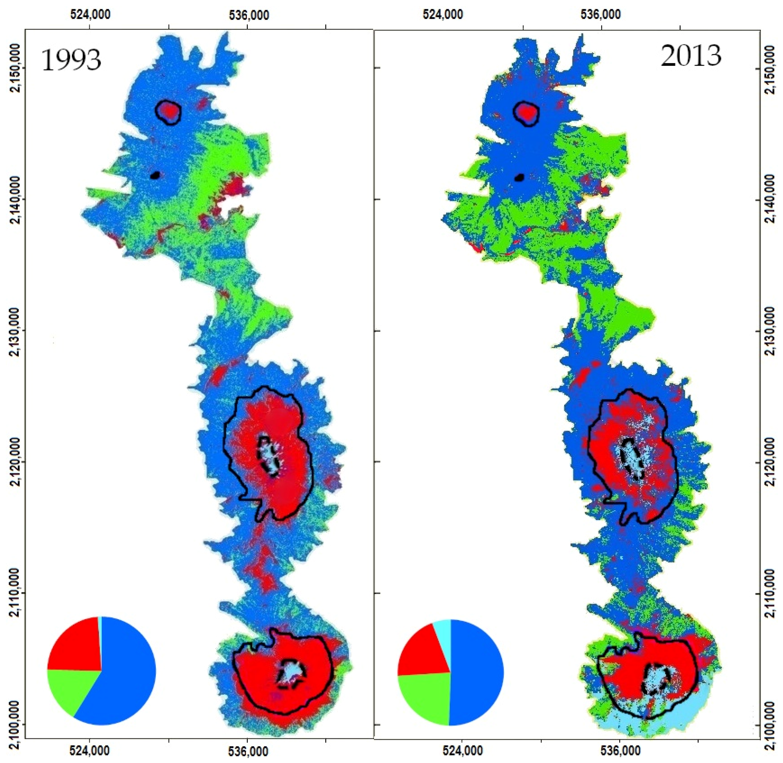
2.2. Remote Sensing-Based Maps

To analyze the spatial variation of P. hartwegii habitat between 1993 and 2013, two Landsat Satellite images were acquired on 5 June 2013 (Sensor 8, Path 26, Row 47, Id: LC80260472013156LGN00) and on 2 September 1993 (Sensors 5, Path 26, Row 47, LT50260471993053AAA04) from the United States Geological Survey [53]. The 30-m resolution images were geo-referenced and atmospherically and geometrically corrected with ground control points using ENVI 4.5 Software (C Exelis Visual Information Solutions, Boulder, Colorado). The images were classified to create supervised vegetation maps of the National Park, for which seven classes were previously defined following Rzedowski (1978) [52] (

Table 1. Predefined classes were previously defined following Rzedowski (1978) [52] to classify the satellite images.

Class	Description
Pine forest	Areas dominated by Pinus hartwegii
Pino-Encino-Oyamel forest	Mixed formations dominated by P. hartwegii, Pinus ayacahuite Ehrenb. ex Schltdl., P. montezumae Lamb., Quercus crassifolia Benth., Quercus laurina M. Martens & Galeotti, and Abies religiosa Kunth Schltdl. et Chamy
Urban zones
Crops
Pastures	Areas dominated by Festuca spp., Camalagrostis tolucensis Trin. ex Steud., Agrostis tolucensis Kunth., and Juniperus montícola Martínez
Clouds	Clouds and glaciers
Shadows

).

The 1993 images were classified by means of the Mahalanobis’ Mínimum distance supervised algorithm, with 70 % of the area ground-truthed [54,55]. The ground-truthing data set was obtained from random polygons selected on Quickbird and Ikonos Satellite images assessed with four field observations obtained in the Western slopes of the Tláloc, Iztaccíhuatl, and Popoctépetl (Figure 1, Table S1) from September 2011–March 2012 (given the significant social unrest in the area and consequent risk of sampling at that time, no more field observation points were visited). The same polygons were used as field-based training areas to classify the 2013 Landsat images.

The accuracy of the 1993 and 2013 classification maps were quantified with the 30% remaining ground-truth for each map (16,345 and 9753 pixels, respectively). The accuracy was assessed with the confusion matrix (matrix indicating accordance of the classified pixels with the ground-truth) and the Kappa’s Statistic (a proxy of the difference between the confusion matrix with a random accordance between the classified map and the ground-truth [55]). All maps were created using the ArcMap 10.1 software [56].

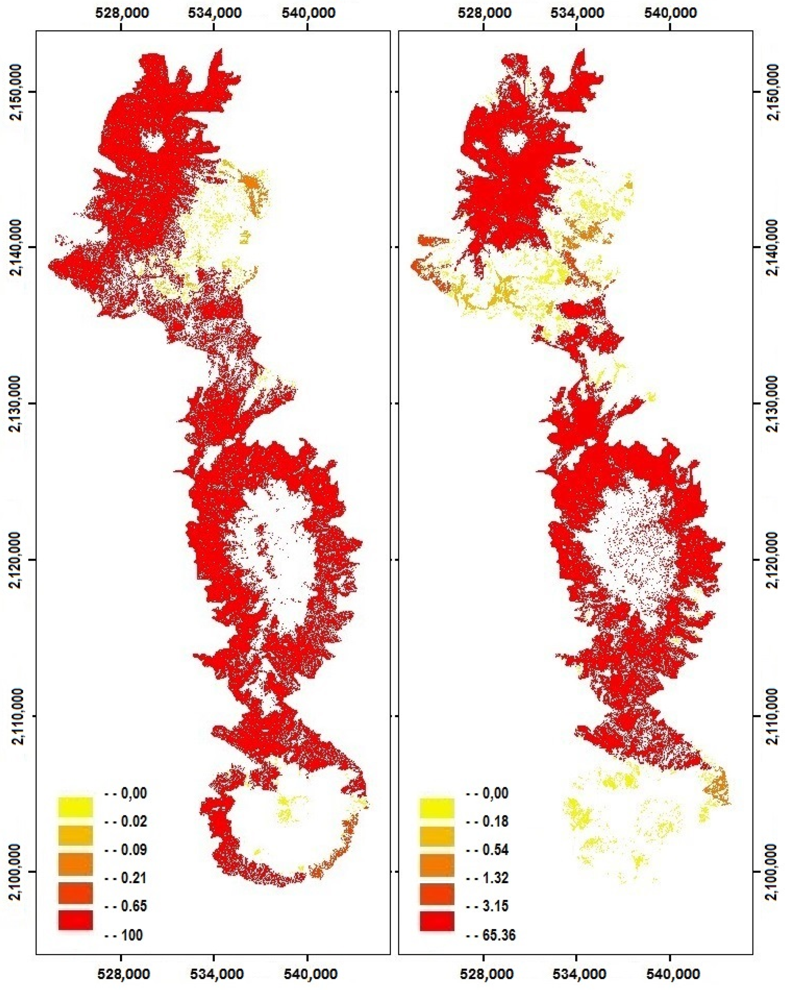
2.3. Changes in Habitat Availability

To assess P. hartwegii habitat changes from 1993 to 2013 in the National Park, we calculated the relative variation of the total habitat (dA):

dA = (A₂₀₁₃ − A₁₉₉₃)/A₁₉₉₃,

(1)

where A_X is the area occupied by the Pine forest class the year _X. A connectivity analysis was performed based on the graph theory [57] as applied by, e.g., [39,43]. Probabilities for every existing link between patches (p_ij) were calculated using two median dispersal distances (19.1 and 52.1 m) to capture the most common range of dispersal variability of pine seeds [58,59,60,61]. Those were obtained from a negative exponential function with a probability value of 0.5 [62].

The change of the total reachable habitat for P. hartwegii (i.e., connected area) was quantified by the relative difference on the Equivalent Connected Area (44) between 1993 and 2013:

dECA = (ECA₂₀₁₃ − ECA₁₉₉₃)/ECA₁₉₉₃,

(2)

calculated for the different pine seed dispersal distances. The Equivalent Connected Area (4), which is obtained from the Probability of Connectivity index (3), represents the size of a hypothetical and unique patch with the same area than the overall reachable habitat for the species in the entire landscape [45,63,64]:

$$\mathrm{PC}=\frac{{{\displaystyle \sum }}_{\mathrm{i}=1}^{\mathrm{n}}{{\displaystyle \sum }}_{\mathrm{j}=1}^{\mathrm{n}}{\mathrm{a}}_{\mathrm{i}}·{\mathrm{a}}_{\mathrm{j}}·{\mathrm{p}}_{\mathrm{ij}}^{*}}{{\mathrm{A}}_{\mathrm{L}}^2},$$

(3)

$$\mathrm{ECA}={\mathrm{A}}_{\mathrm{L}}^2·\surd \mathrm{PC},$$

(4)

where PC is the Probability of Connectivity index, i and j are the source and destination nodes (i.e., habitat patches), a_i and a_j are their attributes (habitat area), n is the total number of patches, ECA is the Equivalent Connected Area, A_L is the maximum landscape attribute, and p*_ij is the probability of connection between patches i and j (considering both direct dispersal or through intermediate stepping stones) [63].

Additionally, the contribution of the different habitat patch to the overall connectivity was portioned into three components [64]:

dPC = dPC_intra + dPC_flux + dPC_conn.

(5)

The intra fraction measures the amount of habitat existing within a particular patch. The flux fraction quantifies how much dispersal flux a patch is expected to receive or produce. Connector fraction (conn) measures the role of a patch as connecting an element or stepping-stone.

All calculations were performed in Conefor 2.6 [65], using habitat area as patch attribute.

2.4. Species Distribution Models

Twenty-four SDMs were fitted for present climate conditions with Maxent software [16,66], combining two sets of current occurrence data (sets 1 and 2) and different complexity by varying the climatic variables, the features allowed in the modeling process, and β-multiplier [17,67].

One hundred Pinus hartwegii natural occurrences (data set 1) from the Mexican Forest Inventory that benefit from an ad-hoc design inventory [50] were used to account for the species’ current presence. To account for a wider ecological native range of P. hartwegii [68], 43 herbarium occurrence records from Guatemala and Honduras [47] were added to the Mexican data to construct the models (Figure 1). Occurrence coincidences in 1-km pixels were aggregated, and ecological outliers were discarded after performing non-metric multidimensional scaling (NMDS) ecological analysis of their annual and seasonal related precipitations and temperatures [69] (Figure S1).

Current climate data for the 1960–1990 period at 30-arc-second (~1 km) resolution were downloaded from the WorldClim 1.4 database [51,70], which provides 19 bioclimatic variables (

Table 2. Wc. V: WorldClim v1.4 climatic variables and their descriptions [51,70]. S1, S2: The two climatic variable sets used to calibrate the model.

Wc. V	Description	S1	S2
BIO 01	Annual Mean Temperature		X
BIO 02	Mean Diurnal Range (Mean of monthly: max temp—min temp)
BIO 03	Isothermality (BIO2/BIO7) (×100)
BIO 04	Temperature Seasonality (standard deviation ×100)
BIO 05	Max Temperature of Warmest Month	X	X
BIO 06	Min Temperature of Coldest Month	X
BIO 07	Temperature Annual Range (BIO5-BIO6)
BIO 08	Mean Temperature of Wettest Quarter	X
BIO 09	Mean Temperature of Driest Quarter	X	X
BIO 10	Mean Temperature of Warmest Quarter
BIO 11	Mean Temperature of Coldest Quarter
BIO 12	Annual Precipitation	X	X
BIO 13	Precipitation of Wettest Month
BIO 14	Precipitation of Driest Month
BIO 15	Precipitation Seasonality (Coefficient of Variation)	X	X
BIO 16	Precipitation of Wettest Quarter
BIO 17	Precipitation Driest Quarter
BIO 18	Precipitation of Warmest Quarter	X
BIO 19	Precipitation of Coldest Quarter		X

) that account for annual trends, seasonality, and extremes in climate that have been reported to act as limiting environmental factors for many organisms [70]. The ecological space of P. hartwegii was defined by 10,000 background points randomly selected in (1) México and (2) Mexico, Honduras, and Guatemala [16] to build all the models.

The selection of climatic variables was based on expert ecological analysis (i.e., stepwise selection following physiologically relevant criteria) [7] among the less correlated variables (Pearson r < 0.75; variance inflation factor < 5) [71,72]. The following options of feature classes provided by Maxent were included in the analysis: “auto-features” (that allow the inclusion of thresholds and hinge features due to physiological limits) and “LQP” (i.e., only linear, quadratic, and product features). Finally, three different β-multipliers, which Maxent uses to control the allowed model complexity, were set: β = 0 (no complexity control), β = 5 (to minimize the complexity of the model), and β = 1 [67].

The models were calibrated with 70% of the occurrence data, after a random selection for set 1 and set 2 data points. The remaining 30% were reserved to perform a non-independent validation [19]: each model was evaluated through the AUC statistic (Area Under the receiver operating characteristic curve), which informs about the ability of the model to discriminate between species’ presences and absences [21,73]. To account for the goodness of fit and the model complexity, the AICc (Akaike Information Criterion corrected for small sample sizes) was also calculated [17,74].

Due to the absence of other available independent data to validate the models, remote sensing data were used as an alternative to evaluate the habitat suitability models. Validation was performed by calculating the Pearson correlation coefficient between the habitat suitability values predicted by each Maxent model in each pixel and the corresponding P. hartwegii occupation percentages calculated from the 2013 RSD-based map (r_HS-PO). To calculate P. hartwegii’s surface occupation at 1-km resolution, the original 30-m P. hartwegii pixeled map was converted to relative percentage occupation on a 1-km² map.

Validation of the habitat suitability models with the RSD-based map was graphically counter-checked with the usual data-partitioning method to visualize agreements between r_HS-PO and AIC. A detailed description of the modelling process can be found in Table S2, following the ODMAP v1.0 standardized protocol for reporting SDM [75]

2.5. Climate Change Impact on P. hartwegii Distribution

As a baseline, the present realized niche (the niche occupation index (NOI)) of P. hartwegii was calculated as the percentage occupation of the suitable area (as calculated from the model with best r_HS-PO and AIC performance). Present species’ occupation was derived from the 2013 P. hartwegii RSD-based map.

To evaluate P. hartwegii habitat suitability changes under different future human-developing scenarios in the study area, the Maxent models were projected to the corresponding climate conditions. We used the reproduction of future climatic conditions from two Earth System Models (ESMs) with three representative CO₂ Concentration pathways (RCP2.6, RCP4.5, and RCP8.5.): NorESM1-M y MPI-ESM-MR [76,77,78]. Among the available ESMs, these were selected after proving to perform well in the region when reproducing present and future climate conditions (see Figures S2 and S3) [79,80]. The values of the bioclimatic variables for the future scenarios were obtained from the WorldClim database for the periods 2050 (2041–2060) and 2070 (2061–2080). This database provides 1-km spatial resolution, after following a delta change-factor approach to downscale the original 2.5° cell size provided by the ESMs for each RCP [81]. To evaluate the sensitivity of P. hartwegii to the forecasted climate change, percentage variations of habitat suitability (HSV) between the present (2013) and the future climate conditions (2050 and 2070) were calculated [82,83].

To calculate NOI and HSV indexes, the suitability maps were converted into binary maps (0: non suitable pixel; 1: suitable pixel) with different suitable thresholds [84,85]. To account for permitted commission and omission errors, four different thresholds were utilized [71,85]: (1) the “Maximum test sensitivity plus specificity” Maxent threshold option (that predicts as absences the 10% of the inventoried presences with the most extreme environmental values), (2) the “10 percentile training presence” (that includes the 90% of the occurrences on the suitable areas), (3) 0.25 habitat suitability threshold, and (4) 0.5 habitat suitability threshold.

Changes in P. hartwegii habitat suitability for the future scenarios were counterchecked with the observed changes on land use from 1993 to 2013, to balance climate change impacts relative to the observed anthropogenic landscape fragmentation.

3. Results

3.1. Remote Sensing Data

The classification of the 1993 and 2013 Landsat images provided a vegetation map of the study area (Figure 2), with a 0.64 and 0.81 Kappa’s statistic, respectively. The 2013 confusion’s matrix showed that the errors were mainly due to confusions between P. hartwegii and the Pino-Encino-Oyamel mixed forest (19.02% and 18.14% misclassified pixels, respectively), and between urban and crop lands (24.60% urban misclassified pixels). The errors on the 1993 vegetation map were due to misclassifications among Pine, Pino-Encino-Oyamel, and pasture classes (19.5, 16.2, and 40.2), and among urban, crops, and snow classes (59.2, 39.8, and 20.5 misclassification percentages).

The 1993 and 2013 vegetation maps show the existence of two large habitat patches of P. hartwegii surrounding the Tláloc and Iztaccíhuatl-Popocatépelt volcanoes (Figure 2). In 1993, the pine forest occupied 58.80% of the National Park, in contrast to 50.59% in 2013, which corresponds to a habitat loss of 14.1%. However, when the connection between patches is taken into account (i.e., Equivalent Connected Area), a reduction of the reachable habitat up to 59.7% and 56.3% was observed for dispersal distances of 19.1 m and 52.7 m, respectively.

Simultaneously, at the expense of the P. hartwegii forest type, habitat increases from 16.57% to 23.42% were detected in the mixed pine forest (Pino-Encino-Oyamel) between 1993 and 2013. This pattern is clearly visible in the surrounding areas of the Popocatépetl volcano, although the area covered by clouds in the south for the 2013 image could be over-enhancing the effect of such change in this area. (Figure 2). Other noticeable changes observed in landcover during this period were related to pastures and crop lands (from 23.54% to 20.32% cover). Surrounding the Iztaccíhuatl volcano, the observed P. hartwegii tree-line decrease on the Western slope between 1993 and 2013 was compensated by an altitudinal gain on the Southern slope (Figure 2).

Regarding the importance of the individual patches to maintain the overall connectivity (dPC), the habitat patches showed a higher density in the north compared to the south of the study area (Figure 3).

When analyzing the ways that patches contributed to maintain the overall connectivity, marked differences in the role of patches were observed in the 20-year span. Besides observing the loss of some connections between patches, a noticeable decrease of the intrapatch connectivity was observed in 2013. Conversely, the contribution of patches as elements of dispersal flux (dPC_flux) and connector elements (dPC_conn) increased in 2013, a trend that is more evident with 52.72-m dispersal distance (

Table 3. Decomposition of dCP (intra, flux, and connector) for the varying dispersal distances D (meters) and years (yr) (5).

Yr	D (m)	dPCintra	dPCflux	dPCconn
1993	19.1	98.79	1.03	0.18
1993	52.72	95.76	3.47	0.76
2013	19.1	94.81	4.67	0.52
2013	52.72	77.29	17.80	4.91

).

Additionally, a relative decrease of dA = −14.15% (1) was observed on P. hartwegii habitat between 1993 and 2013. The relative variation of the total reachable habitat between 1993 and 2013 (dECA = −59.7% and −56.3% for dispersal distances of 19.10 and 52.72 m, respectively) and (2) evidenced the levered effect of the anthropogenic habitat fragmentation on the habitat loss.

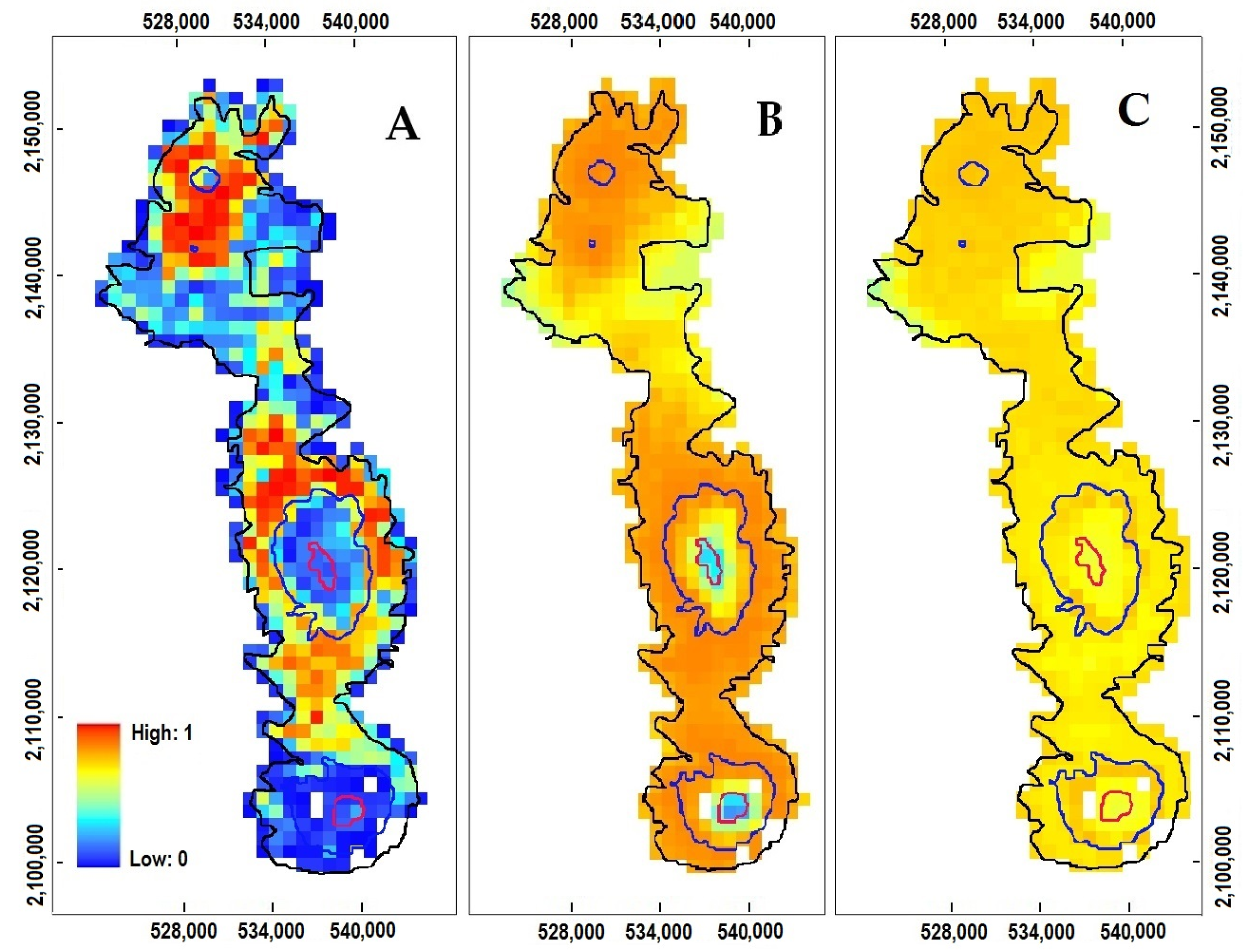
3.2. P. hartwegii Habitat Suitability Models

After aggregating duplicated data, removing outliers and poorly georeferenced data, and performing the non-metric multidimensional scaling ecological analysis (Figure S1), 97 P. hartwegii natural occurrences from the Mexican Forest Inventory were used in the analysis as data set 1. The additional herbarium data from Honduras and Guatemala comprised 121 occurrences and were used as data set 2 (Figure 1A). As independent variables to explain the occurrence data, two sets of WorldClim climatic variables were selected after correlation and expert-based analysis (Table 2).

The standard cross evaluation of the 24 fitted Maxent models showed similar AUC values above 0.98. Small differences were observed between the models calibrated with the Mexican data set (0.9805 to 0.9888 AUC) and the models performed with the world’s distribution data set (0.9919 to 0.9942 AUC) (

Table 4. Characterization of the different distribution models. Model Id.: Identification number of the model). Occ: Occurrence data (97 Mexican occurrences. 24 Guatemala and Honduras occurrences). n: number of independent variables included in the model. Features: features classes allowed in the modeling process. L.Q.P: Linear, quadratic and product features. β: Maxent β-multiplier. AUC: Area Under the receiver operating characteristic curve. AIC: Akaike Information Criterion corrected for small sample sizes. p: number of parameters of each model. r_HS-PO: Spearman correlation between habitat suitability values (HS) and the percentage occupation (PO) of P. hartwegii on the 2013 satellite derived map. Shadowed in gray: best and worst model r_HS-PO model. Bold: best models.

Model Id.	Occ.	n	Features	β	AUC	AIC	p	rHS-PO
1	121	7	Auto-features	0	0.981	-	159	0.180
2	121	7	Auto-features	1	0.986	3274.54	33	0.395
3	121	7	Auto-features	5	0.986	2908.33	14	0.403
4	121	7	L.Q.P	0	0.988	2846.66	12	0.443
5	121	7	L.Q.P	1	0.988	2839.50	10	0.446
6	121	7	L.Q.P	5	0.988	2858.54	8	0.421
13	121	6	Auto-features	0	0.981	-	140	0.233
14	121	6	Auto-features	1	0.988	2960.42	28	0.363
15	121	6	Auto-features	5	0.988	2868.96	9	0.330
16	121	6	L.Q.P	0	0.988	2867.29	12	0.357
17	121	6	L.Q.P	1	0.989	2861.54	7	0.343
18	121	6	L.Q.P	5	0.989	2868.03	6	0.321
7	97	7	Auto-features	0	0.994	3071.03	79	0.340
8	97	7	Auto-features	1	0.994	2369.42	18	0.213
9	97	7	Auto-features	5	0.994	2257.98	11	0.325
10	97	7	L.Q.P	0	0.994	2276.60	14	0.351
11	97	7	L.Q.P	1	0.993	2322.88	9	0.397
12	97	7	L.Q.P	5	0.993	2279.90	8	0.381
19	97	6	Auto-features	0	0.992	2688.57	69	0.240
20	97	6	Auto-features	1	0.992	2282.71	18	0.153
21	97	6	Auto-features	5	0.992	2279.01	8	0.225
22	97	6	L.Q.P	0	0.993	2284.95	11	0.342
23	97	6	L.Q.P	1	0.992	2313.13	9	0.285
24	97	6	L.Q.P	5	0.992	2333.28	5	0.265

). Focusing on the RSD-based validation index (r_HS-PO) of the models differing only from the occurrence data set, better models were also observed on those calibrated with Mexican data (data set 1).

The AIC, considering both the complexity (number of parameters) and the goodness of fit of the models, showed varying penalization when using different combinations of occurrence data sets and complexity (Table 4).

The models’ performance with the world’s occurrence data set (set 2), after removing the most complex model, showed AIC ranging from 2839.50 to 3274.54 (Table 4). When removing the three models with AIC higher than 3000, an inverse relationship trend can be seen between AIC and the RSD-based validation index (r_HS-PO) (see Figure S4). Model 5, which was performed with seven climatic variables (see weights in Table S2), LQP features, and β-multiplier =1, resulted to be the best model among those performed with the set 2 of P. hartwegii occurrences (see Table 4). When comparing the choices to perform the models, the auto-feature option had the worst performance compared to the models restricted to only linear, quadratic, and products relationships (L.Q.P.). However, within the auto-feature selection, the models improved when restricting complexity (β = 1 or 5) and reducing the independent climatic variables to six.

Similarly, the AIC ranged from 2257.98 to 3071.03 on the models performed with the Mexican data set (set 1) (Table 4). In this case, the best model differed when taking AIC or r_HS-PO into consideration (being models 9 and 11 the best ones, respectively). Better models were those performed with seven independent variables and two choices to control the complexity of the model: no mathematical control (i.e., auto-features) but maximum control with β-multiplier (β = 5), or mathematic relationships restricted to L.Q.P with an intermediate β-multiplier control (β = 1). Parallel to the world’s occurrence data set, an inverse trend between both validation parameters (AIC and r_HS-PO) was observed on the Mexican data set, after removing the most complex models with an AIC > 3000 (Figure S4).

The three best models (5, 9, and 11), the ones performed with the world’s occurrence data set, L.Q.P. features, and intermediate β control (=1), showed better r_HS-PO correlation (≥0.40) than the one performed with auto-features compensated with β = 5 and the occurrence data restricted to Mexico. The worst model derived from the RSD-based validation index was model 20, which, surprisingly, did not show a poor AIC (Table 4). This model was performed with the most restricted occurrence data and climatic variables, auto-features, and an intermediate β control. Within the best model (model 5), the weights of the climatic variables showed Bio 5 (Maximum temperature of the warmest month) to be the most important variable, with 94.4% contribution in the worst model (See Table S2). However, the best model showed other temperature variables to complement Bio 5 information with an additional 15.8% of model performance.

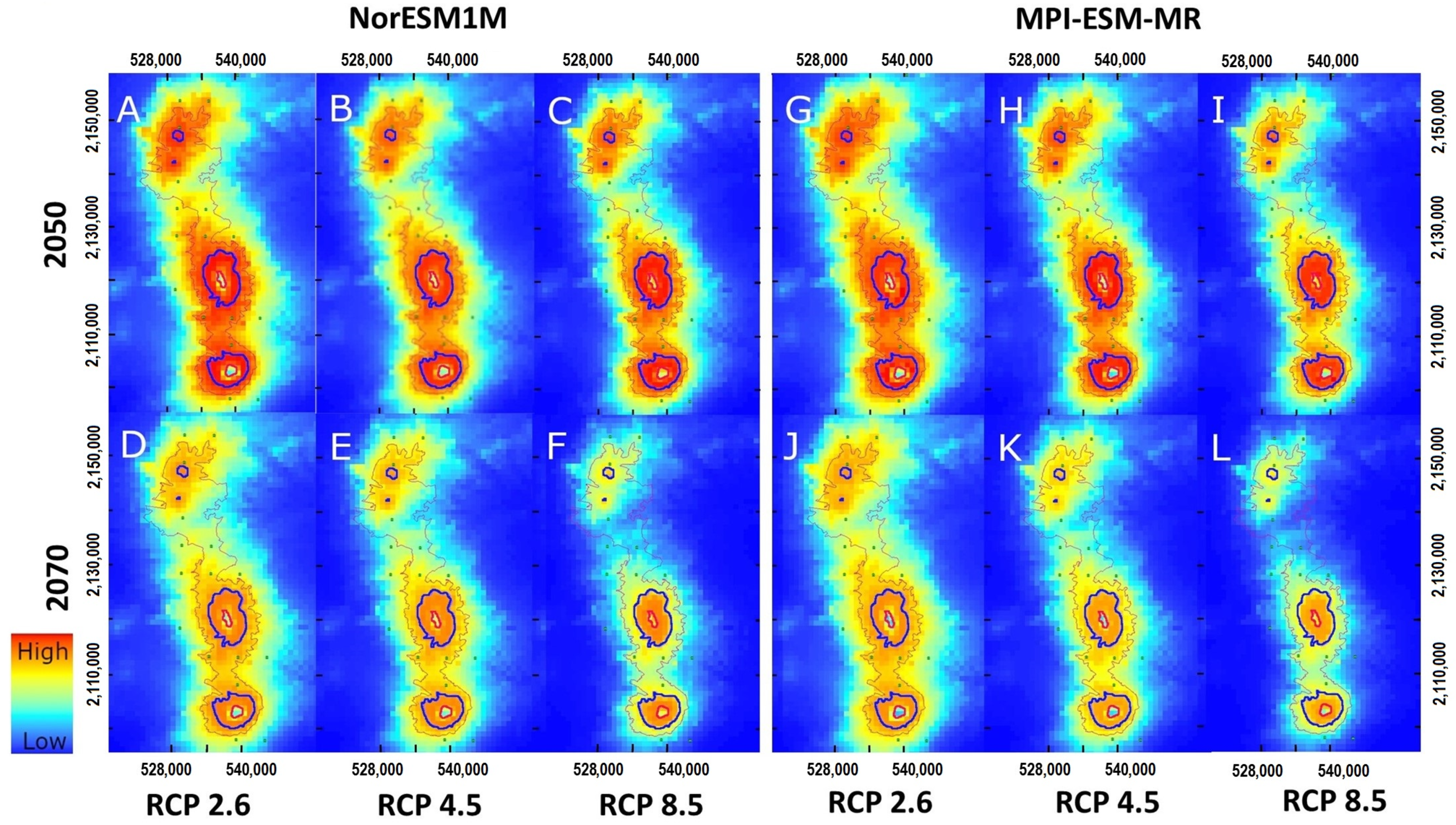
3.3. Projections to Present and Future Climate Conditions

Projections of P. hartwegii habitat suitability to present climate conditions of the best and worst RSD validated models (models 5 and 20; Figure 4B,C) showed contrasting agreements with the 2013 RSD-based P. hartwegii occupation map (Figure 4A). This reinforces the importance of calibrating models with different complexity, followed by a validation process best performed with independent occurrence data. Model 5 (Figure 4B) showed a high P. hartwegii habitat suitability except for the valley between Tláloc and Iztaccíhuatl volcanoes and the Iztaccíhuatl and Popocatépetl summits. No inferences can be made from the visual disagreements between the 2013 RSD occupation map and the model 5 habitat suitability projection on the Popocatépetl southern slope (bottom of Figure 4A), as this part of the satellite image was covered with clouds (see Figure 2, right).

As the baseline, niche occupation index (NOI) varied between 47.81% and 49.28% depending on the different threshold options for present climate conditions. The worst, 47.81%, occupation index was performed with 0.5 probability threshold, while for 0.25, a 10-percentile presence (10p), maximum training sensitivity plus specificity (max), and NOI between 49.08 and 49.28 were observed.

Projections of model 5 to 2050 future climate conditions showed an increased P. hartwegii habitat suitability in Izta Popo National Park, however, decreasing its suitability as the CO₂ emission scenarios worsens (from RCP 2.6 to RCP 8.5). The decrease in habitat suitability is clearly observed on the lowest areas, somehow counterbalanced with increases in the summits of the National Park. Projections to 2070 show the same pattern, although with worse suitability values (Figure 5).

Focusing on the 0.5 suitability threshold and 2050, habitat decreases from 5.94% to 23.19% were observed in the Habitat Suitability Variation index (HSV) for the varying scenarios. The remaining threshold options did not show any significant variation for the 2050 projections. The 2070 projections showed relevant increases in habitat losses in every different threshold except for “Maximum test sensitivity plus specificity”, which remained flat (Table S3). The 0.5 threshold showed habitat losses from 6.35% (RCP 2.6) to 43.74% (RCP 8.5). Between the two climatic models, MPI-ESM-MR showed higher climate change impact on the P. hartwegii habitat suitability, except for RCP 2.6, where similar values were observed (Table S3).

4. Discussion

The integration of RSD, SDMs, and connectivity metrics provide a powerful tool to assess the impact of climate change and anthropogenic land conversion that are the main drivers impacting biological systems [1]. Although the use of RSD to generate predictor variables is becoming more common in SDM, its potential as a validation tool in areas with poor field data remains relatively unexplored. Furthermore, RSD can be particularly valuable to assess ecological networks, by quantifying habitat connectivity levels and characterizing priorities to maintain connectivity.

4.1. The Use of Remote Sensing Data to Validate Species Distribution Models

The use of RSD to validate vegetation models and identify vegetation types has been useful at large scales (e.g., 0.5° resolution) [86]. However, its use to validate SDM at higher scales (e.g., 1-km² resolution) is rare, as identifying species from remote sensing data is not straightforward. First experiences to identify individual tree species confirmed the high value of RSD, thanks to the increasing availability of higher-resolution images at high frequency [28,87,88]. Parallel efforts to generate ground data [50] provide fundamental knowledge to get better accuracy on RSD-based maps [22]. As RSD classification maps are assessed by “ground-truthing” [55], obtaining accurate field data is key to getting accurate species distribution maps. This is particularly relevant in areas with steep environmental gradients with corresponding high vegetation cover diversity, such as mountain areas. In these zones, ecological data are usually biased towards lower altitudes, whose limitations are added to constraints of climatic models that are usually based on few stations at low altitudes (e.g., see available meteorological stations for the study area in Figure 1B) [33,89].

In our case study, due to the monospecific forests of P. hartwegii, the presence maps at 1-km resolution obtained from the 1993 and 2013 RSD can be used with good confidence (Kappa’s index > 0.6) [90]. The 0.81 accuracy of the 2013 map makes it a valuable map to assess the effect of the different calibration options on the predictive ability of the fitted P. hartwegii habitat suitability models. Although the Kappa’s accuracy of the 1993 remote sensing map is relatively lower (0.64), its errors are majorly attributed to misclassification of urban, crop lands, pastures, and snow classes. This map, however, is used only to evaluate land use fragmentation and connectivity changes.

4.2. Species Distribution Modeling

The higher RSD-based validation index r_HS-PO shown by the models run with global presence data set compared with those run with the Mexican data (0.38 ± 0.05 vs. 0.29 ± 0.07; Table 4) agrees with previous studies that conclude that performing habitat suitability models with the species’ full ecological range achieve better results in model calibration [5,67,68]. This is best observed on the environmental envelopes (NMDS) performed on both data sets; these show how P. hartwegii environmental conditions from Guatemala and Honduras complement the climatic spectrum provided by the Mexican occurrences (see e.g., Annual precipitation in Figure S1B). This conclusion supports the recommendations made by other authors to perform environmental envelope analysis, ensuring the meeting of the niche space assumption (i.e., full range of abiotic conditions are contained) [9,67].

Secondly, the trends observed in the RSD-based model assessment and the AIC agree with previous studies that indicate that models with intermediate complexity are more robust [17,67]. In this case study, the best models were achieved either by relaxing the Maxent β complexity (β > 0) or alternatively reducing the allowed function features (to L,Q,P).

Regarding the number of explanatory variables to fit the models, we followed the advice of many authors who recommend a previous stepwise selection of those variables to avoid the negative effects of auto-correlation [67,91,92,93]. In our study area, key climatic variables regarding the duration and amplitude of cold and dry seasons [7] and leaving more variables in the model produced slightly better models.

The small differences observed in AUC for the different Maxent models, compared with the contrasting AIC and RSD-based validation indexes, could be a consequence of using the same data for training and validating the model, which could be partially solved using a spatial data-partitioning method to train and validate the model [20,71]. The small difference in AUC also agrees with other studies that state that AUC ignores the goodness of fit of the models and provides very high values when the extension of the species’ distribution is much smaller than the geographical area of the study [21,90].

In contrast, the RSD-based validation method proposed in this study has advantages over AUC and AIC, as it emerges from a completely independent data source and can compare the accuracy of models independently using varying calibration options (data sets, geographical amplitude, backgrounds) [21,94]. The coincidence of the best model as selected from the RSD validation index and the AIC from those fitted with the world’s data set stands as evidence of the validity of the proposed remote sensing-based validation method.

4.3. Impact of Cover Change on Habitat Availability and Reachability

The noticeable P. hartwegii forest decrease (14.15%) observed from 1993 to 2013 aligns with anthropogenic impact [95,96]. To analyze the effect of this loss in the habitat connectivity, the dispersal ability of the species (a key functional element joining pairs of nodes [57]) needs to be estimated. However, dispersal capability is a complex process that depends on many factors (e.g., tree density, location, seed production, dispersal, fecundity, and establishment) [59] that remains largely unexplored in plants [58,60,61]. Although specific data on the species’ movement should ideally be used, the two dispersal distances here considered to cover the most common range of dispersal ability in other Pinus species [58,59,60,61] showed similar declines of P. hartwegii habitat connectivity from 1993 to 2013 (56.3–59.7%). This dramatic decrease suggests a loss of key habitat patches for the ecological functionality of the species. The decrease of each patch contribution over the probability of connectivity index (dPC_intra) along the studied time period suggested that the species lost large habitat patches (that provided significant amount of intrapatch connectivity in 1993). Consequently, the ecological network shifted in 2013 to a greater reliance on the remaining patches as a connecting stepping stone (dPC_conn) and as patches receiving or producing dispersion (dPC_flux). This pattern of habitat loss and fragmentation may jeopardize the flux and the strength of connections to other patches, raising the question of the capability of isolated patches to maintain populations with low dispersal capacity, such as those associated with P. hartwegii [97]. Habitat change is more acute in the north and south of the National Park (Figure 2), with a remarkable connectivity drop between the Tláloc and Iztaccíhuatl summits (Figure 3), where the remaining fragments cannot compensate for the decrease of connectivity and the increasing patchiness of the populations. These findings document that the conservation of specific habitat patches can be critical to maintain habitat functionality and that management efforts should focus on their conservation.

4.4. The Impact of Climate Change

As a baseline, a niche occupation index (NOI) between 47.81% and 49.28% (i.e., habitat occupation of its suitable area) in 2013 documents the limitations to occupy all areas that are abiotically suitable for P. hartwegii. Anthropogenic impact, demography, and dispersal constraints, together with biotic interactions, stochastic events, and historical aspects, are among the responsible factors [9,90].

Illegal logging evidenced even during fieldwork and the extensive cattle industry [98,99] point to anthropogenic impacts as a main driver of the observed landscape fragmentation from 1993 to 2013 (see Figure 3). The contrasting increase of the mixed pine forest at the expense of P. hartwegii monospecific forest could be a response of its intense extraction and its natural replacement by other species (e.g., Pinus patula Schiede ex Schltdl. & Cham., Quercus crassipes Bonpl., Quercus laurina Bonpl., Abies religiosa (Kunth) Schltdl. & Cham.) to provide further challenges. At the upper tree line, pastures can replace P. hartwegii forest under such uncontrolled logging as observed in the Western slope of Iztaccíhuatl volcano (Figure 2).

In line with numerous studies that show an altitudinal and latitudinal shift of species’ ranges in response to past and forecasted climate changes [100,101,102,103], the projections to future climate conditions show a clear tendency of P. hartwegii to migrate up-slope (Figure 5). The observed tendency is visible when comparing the habitat suitability under present (Figure 4B) and future climate conditions (Figure 5) between the Tláloc and the Iztaccíhuatl volcanoes, and above 4000 m a.s.l., which project a clear reduction of the habitat suitability in 2070.

Although the quantification of the total loss of suitable area is highly dependent on the threshold used to transform a continuous map into a binary map (see HSV index in Table S2) [85], it gives evidence of the worrying effect of the greenhouse effect as RCP become more extreme; e.g., up to a 32–43.7% of habitat loss was observed in the 2070 projections using the 0.5 threshold option. This tendency aligns with the observed and modeled climatic shifts [79,80], which show increases of maximum and minimum temperatures of up to 3.2 °C by 2085 (Figure S2). The essential temperature dependency of habitat suitability models in mountain environments (see Table S2) continues to be a concern under warming global climates.

Challenges related to deforestation, fire, and climate change have already been pointed as being critical in Mexico [98]. Several projects have been launched by the Mexican Government and wider partnerships to assess the value of the Izta Popo ecosystem services and to ensure the wider sustainability of the National Park [99]. The specific Payments of Environmental Services Schemes put forward (i.e., voluntary transaction in which a user buys a specific ecosystem service [98], or the planting of 300,000 P. hartwegii seedlings above 4000 m a.s.l. in Izta-Popo [104]) are good examples of responses at a National level to preserve the ecosystem and associated services threatened by land use and forecasted climate change evidenced by this study. Other actions aimed to adapt ecosystems to climate change (e.g., assisted migration of pine for successful colonization [99]), could benefit from the connectivity analysis presented here to focus ecological restoration in key areas.

5. Conclusions

To overcome limitations of field-based observations in areas that are difficult to monitor or unsafe areas, the incorporation of RSD with SDM can be a useful tool to assess vegetation change. RSD have been incorporated into the modeling procedure as an independent validation tool to test SDM performance.

The contrasting geographical projections of the P. hartwegii habitat suitability modeled to present conditions point out that during the modeling process there are important decisions to be made. Contrary to other validation methods, using RSD offers the advantage to evaluate different models independently.

Anthropogenic pressures on the Izta Popo National Park have led to a reduction of P. hartwegii forest cover and a drastic drop in its connectivity from 1993 to 2013. During these 20 years a significant number of critical elements for connectivity have disappeared, forcing a shift of the ecological network of the species to rely on weaker connections between habitat patches. Undertaking a detailed node analysis could determine the priority areas that conservation would ensure the habitat connectivity maintenance.

There is a reduction of P. hartwegii habitat suitability under climate projections for 2050 and 2070 parallel to an upslope shift in its altitudinal range. This trend, which is more acute as CO₂ scenarios worsen, can results in the split of the 2013 continuous suitable area of the species into separate patches. Climate change impacts aggravate the anthropogenic fragmentation process that the National Park suffered from 1993 to 2013, with impact on ecosystem services (water supply, carbon storage, diversity conservation, etc.). These shifts on P. hartwegii ecosystem ultimately impact on the livelihoods of the communities that live around the Izta Popo National Park as well as down-stream communities and the wider nation.

References

1. Shukla, P.; Skea, J.; Calvo Buendia, E.; Masson-Delmotte, V.; Pörtner, H.; Roberts, D.; Zhai, P.; Slade, R.; Connors, S.; Van Diemen, R. IPCC, 2019: Climate Change and Land: An IPCC Special Report on Climate Change, Desertification, Land Degradation, Sustainable Land Management, Food Security, and Greenhouse Gas Fluxes in Terrestrial Ecosystems; Report; Intergovernmental Panel on Climate Change (IPCC): Geneva, Switzerland, 2019; pp. 1–864. [Google Scholar]
2. Foden, W.B.; Young, B.E.; Akçakaya, H.R.; Garcia, R.A.; Hoffmann, A.A.; Stein, B.A.; Thomas, C.D.; Wheatley, C.J.; Bickford, D.; Carr, J.A.; et al. Climate change vulnerability assessment of species. Wiley Interdiscip. Rev. Clim. Chang. 2019, 10, 551. [Google Scholar] [CrossRef] [Green Version]
3. Pederson, G.T.; Graumlich, L.J.; Fagre, D.B.; Kipfer, T.; Muhlfeld, C.C. A Century of Climate and Ecosystem Change in Western Montana: What Do Temperature Trends Portend? Clim. Change 2010, 98, 133–154. [Google Scholar] [CrossRef]
4. Kohler, T.; Giger, M.; Hurni, H.; Ott, C.; Wiesman, U.; von Dach, S.W.; Maselli, D. Mountains and Climate Change: A Global Concern. Mt. Res. Dev. 2010, 30, 53–55. [Google Scholar] [CrossRef] [Green Version]
5. Titeux, N.; Maes, D.; Van Daele, T.; Onkelinx, T.; Heikkinen, R.K.; Romo, H.; García-Barros, E.; Munguira, M.L.; Thuiller, W.; van Swaay, C.A. The Need for Large-scale Distribution Data to Estimate Regional Changes in Species Richness under Future Climate Change. Divers. Distrib. 2017, 23, 1393–1407. [Google Scholar] [CrossRef] [Green Version]
6. Pearson, R.G.; Dawson, T.P.; Berry, P.M.; Harrison, P. Species: A Spatial Evaluation of Climate Impact on the Envelope of Species. Ecol. Model. 2002, 154, 289–300. [Google Scholar] [CrossRef]
7. Pearson, R.G.; Dawson, T.P. Predicting the Impacts of Climate Change on the Distribution of Species: Are Bioclimate Envelope Models Useful? Glob. Ecol. Biogeogr. 2003, 12, 361–371. [Google Scholar] [CrossRef] [Green Version]
8. Bambach, N.; Meza, F.J.; Gilabert, H.; Miranda, M. Impacts of Climate Change on the Distribution of Species and Communities in the Chilean Mediterranean Ecosystem. Reg. Environ. Change 2013, 13, 1245–1257. [Google Scholar] [CrossRef]
9. Anderson, R.P. A Framework for Using Niche Models to Estimate Impacts of Climate Change on Species Distributions. Ann. N. Y. Acad. Sci. 2013, 1297, 8–28. [Google Scholar] [CrossRef]
10. Jiménez-Valverde, A.; Acevedo, P.; Barbosa, A.M.; Lobo, J.M.; Real, R. Discrimination Capacity in Species Distribution Models Depends on the Representativeness of the Environmental Domain. Glob. Ecol. Biogeogr. 2013, 22, 508–516. [Google Scholar] [CrossRef] [Green Version]
11. Peterson, A.; Soberón, J. Interpretation of Models of Fundamental Ecological Niches and Species Distribution Areas. Biodivers. Inform. 2005, 2, 1–10. [Google Scholar] [CrossRef] [Green Version]
12. Elith, J.; Leathwick, J.R. Species Distribution Models: Ecological Explanation and Prediction across Space and Time. Annu. Rev. Ecol. Evol. Syst. 2009, 40, 677–697. [Google Scholar] [CrossRef]
13. Guisan, A.; Zimmermann, N.E. Predictive Habitat Distribution Models in Ecology. Ecol. Model. 2000, 135, 147–186. [Google Scholar] [CrossRef]
14. Mateo, R.G.; Felicisimo, A.M.; Munoz, J. Species Distributions Models: A Synthetic Revision. Rev. Chil. Hist. Nat. 2011, 84, 217–240. [Google Scholar] [CrossRef] [Green Version]
15. Yates, K.L.; Bouchet, P.J.; Caley, M.J.; Mengersen, K.; Randin, C.F.; Parnell, S.; Fielding, A.H.; Bamford, A.J.; Ban, S.; Barbosa, A.M. Outstanding Challenges in the Transferability of Ecological Models. Trends Ecol. Evol. 2018, 33, 790–802. [Google Scholar] [CrossRef] [Green Version]
16. Phillips, S.J.; Dudík, M. Modeling of Species Distributions with Maxent: New Extensions and a Comprehensive Evaluation. Ecography 2008, 31, 161–175. [Google Scholar] [CrossRef]
17. Warren, D.L.; Seifert, S.N. Ecological Niche Modeling in Maxent: The Importance of Model Complexity and the Performance of Model Selection Criteria. Ecol. Appl. 2011, 21, 335–342. [Google Scholar] [CrossRef] [Green Version]
18. Zhu, G.; Qiao, H. Effect of the Maxent model’s complexity on the prediction of species potential distributions. Biodivers. Sci. 2016, 24, 1189–1196. [Google Scholar] [CrossRef] [Green Version]
19. Araújo, M.B.; Pearson, R.G.; Thuiller, W.; Erhard, M. Validation of Species–Climate Impact Models under Climate Change. Glob. Chang. Biol. 2005, 11, 1504–1513. [Google Scholar] [CrossRef] [Green Version]
20. Muscarella, R.; Galante, P.J.; Soley-Guardia, M.; Boria, R.A.; Kass, J.M.; Uriarte, M.; Anderson, R.P. ENM Eval: An R Package for Conducting Spatially Independent Evaluations and Estimating Optimal Model Complexity for Maxent Ecological Niche Models. Methods Ecol. Evol. 2014, 5, 1198–1205. [Google Scholar] [CrossRef]
21. Lobo, J.M.; Jiménez-Valverde, A.; Real, R. AUC: A Misleading Measure of the Performance of Predictive Distribution Models. Glob. Ecol. Biogeogr. 2008, 17, 145–151. [Google Scholar] [CrossRef]
22. Ahrends, A.; Bulling, M.T.; Platts, P.J.; Swetnam, R.; Ryan, C.; Doggart, N.; Hollingsworth, P.M.; Marchant, R.; Balmford, A.; Harris, D.J. Detecting and Predicting Forest Degradation: A Comparison of Ground Surveys and Remote Sensing in Tanzanian Forests. Plants People Planet 2021, 3, 268–281. [Google Scholar] [CrossRef]
23. Cord, A.F.; Brauman, K.A.; Chaplin-Kramer, R.; Huth, A.; Ziv, G.; Seppelt, R. Priorities to Advance Monitoring of Ecosystem Services Using Earth Observation. Trends Ecol. Evol. 2017, 32, 416–428. [Google Scholar] [CrossRef]
24. Iverson, L.R.; Graham, R.L.; Cook, E.A. Applications of Satellite Remote Sensing to Forested Ecosystems. Landsc. Ecol. 1989, 3, 131–143. [Google Scholar] [CrossRef]
25. McRoberts, R.E.; Wendt, D.G.; Nelson, M.D.; Hansen, M.H. Using a Land Cover Classification Based on Satellite Imagery to Improve the Precision of Forest Inventory Area Estimates. Remote Sens. Environ. 2002, 81, 36–44. [Google Scholar] [CrossRef]
26. Chirici, G.; Mura, M.; McInerney, D.; Py, N.; Tomppo, E.O.; Waser, L.T.; Travaglini, D.; McRoberts, R.E. A Meta-Analysis and Review of the Literature on the k-Nearest Neighbors Technique for Forestry Applications That Use Remotely Sensed Data. Remote Sens. Environ. 2016, 176, 282–294. [Google Scholar] [CrossRef]
27. Viña, A.; Gitelson, A.A.; Nguy-Robertson, A.L.; Peng, Y. Comparison of Different Vegetation Indices for the Remote Assessment of Green Leaf Area Index of Crops. Remote Sens. Environ. 2011, 115, 3468–3478. [Google Scholar] [CrossRef]
28. Recuero, L.; Litago, J.; Pinzón, J.E.; Huesca, M.; Moyano, M.C.; Palacios-Orueta, A. Mapping Periodic Patterns of Global Vegetation Based on Spectral Analysis of NDVI Time Series. Remote Sens. 2019, 11, 2497. [Google Scholar] [CrossRef] [Green Version]
29. Reyer, C.P.O.; Silveyra Gonzalez, R.; Dolos, K.; Hartig, F.; Hauf, Y.; Noack, M.; Lasch-Born, P.; Rötzer, T.; Pretzsch, H.; Meesenburg, H.; et al. The Profound Database for Evaluating Vegetation Models and Simulating Climate Impacts on European Forests. Earth Syst. Sci. Data 2020, 12, 1295–1320. [Google Scholar] [CrossRef]
30. Matasci, G.; Hermosilla, T.; Wulder, M.A.; White, J.C.; Hobart, G.W.; Zald, H.S.J.; Coops, N.C. A Space-Time Data Cube: Multi-Temporal Forest Structure Maps from Landsat and Lidar. In Proceedings of the 2017 IEEE International Geoscience and Remote Sensing Symposium (IGARSS); IEEE: Piscataway, NJ, USA, 2017; pp. 2581–2584. [Google Scholar] [CrossRef]
31. Cord, A.F.; Klein, D.; Gernandt, D.S.; de la Rosa, J.A.P.; Dech, S. Remote Sensing Data Can Improve Predictions of Species Richness by Stacked Species Distribution Models: A Case Study for Mexican Pines. J. Biogeogr. 2014, 41, 736–748. [Google Scholar] [CrossRef]
32. West, A.M.; Evangelista, P.H.; Jarnevich, C.S.; Young, N.E.; Stohlgren, T.J.; Talbert, C.; Talbert, M.; Morisette, J.; Anderson, R. Integrating Remote Sensing with Species Distribution Models; Mapping Tamarisk Invasions Using the Software for Assisted Habitat Modeling (SAHM). J. Vis. Exp. 2016, 116, e54578. [Google Scholar] [CrossRef] [PubMed] [Green Version]
33. Pinto-Ledezma, J.N.; Cavender-Bares, J. Using Remote Sensing for Modeling and Monitoring Species Distributions. In Remote Sensing of Plant Biodiversity; Cavender-Bares, J., Gamon, J., Townsend, P., Eds.; Springer: New York, USA, 2020; pp. 199–233. [Google Scholar]
34. de Araujo Barbosa, C.C.; Atkinson, P.M.; Dearing, J.A. Remote Sensing of Ecosystem Services: A Systematic Review. Ecol. Indic. 2015, 52, 430–443. [Google Scholar] [CrossRef]
35. Defries, R.S.; Hansen, M.C.; Townshend, J.R.G.; Janetos, A.C.; Loveland, T.R. A New Global 1-Km Dataset of Percentage Tree Cover Derived from Remote Sensing. Glob. Change Biol. 2000, 6, 247–254. [Google Scholar] [CrossRef]
36. Durán-Medina, E.; Mas, J.F.; Velázquez, A. Cambios En Las Coberturas de Vegetación y Usos Del Suelo En Regiones Con Manejo Forestal Comunitario y Áreas Naturales Protegidas de México. In Los Bosques Comunitarios de México: Manejo Sustentable de Paisajes Forestales; Barton Bray, D., Merino Pérez, L., Barry, D., Eds.; Instituto Nacional de Ecología: Ciudad de México, México, 2007; pp. 267–299. [Google Scholar]
37. Dyke, A.S. Late Quaternary Vegetation History of Northern North America Based on Pollen, Macrofossil, and Faunal Remains. Géogr. Phys. Quat. 2005, 59, 211–262. [Google Scholar] [CrossRef] [Green Version]
38. Reese, H.; Nilsson, M.; Sandström, P.; Olsson, H. Applications Using Estimates of Forest Parameters Derived from Satellite and Forest Inventory Data. Comput. Electron. Agric. 2002, 37, 37–55. [Google Scholar] [CrossRef] [Green Version]
39. Tian, F.; Brandt, M.; Liu, Y.Y.; Rasmussen, K.; Fensholt, R. Mapping Gains and Losses in Woody Vegetation across Global Tropical Drylands. Glob. Chang. Biol. 2017, 23, 1748–1760. [Google Scholar] [CrossRef]
40. Cisneros-Araujo, P.; Ramirez-Lopez, M.; Juffe-Bignoli, D.; Fensholt, R.; Muro, J.; Mateo-Sánchez, M.C.; Burgess, N.D. Remote Sensing of Wildlife Connectivity Networks and Priority Locations for Conservation in the Southern Agricultural Growth Corridor (SAGCOT) in Tanzania. Remote Sens. Ecol. Conserv. 2021, 7, 430–444. [Google Scholar] [CrossRef]
41. Crooks, K.R.; Sanjayan, M.A. Connectivity Conservation: Maintaining Connections for Nature; Cambridge University Press: Cambridge, UK, 2006; pp. 1–20. [Google Scholar]
42. Osipova, L.; Okello, M.M.; Njumbi, S.J.; Ngene, S.; Western, D.; Hayward, M.W.; Balkenhol, N. Using Step-Selection Functions to Model Landscape Connectivity for African Elephants: Accounting for Variability across Individuals and Seasons. Anim. Conserv. 2019, 22, 35–48. [Google Scholar] [CrossRef]
43. de la Fuente, B.; Mateo-Sánchez, M.C.; Rodríguez, G.; Gastón, A.; de Ayala, R.P.; Colomina-Pérez, D.; Melero, M.; Saura, S. Natura 2000 Sites, Public Forests and Riparian Corridors: The Connectivity Backbone of Forest Green Infrastructure. Land Use Policy 2018, 75, 429–441. [Google Scholar] [CrossRef]
44. Zeller, K.A.; McGarigal, K.; Whiteley, A.R. Estimating Landscape Resistance to Movement: A Review. Landsc. Ecol. 2012, 27, 777–797. [Google Scholar] [CrossRef]
45. Saura, S.; Estreguil, C.; Mouton, C.; Rodríguez-Freire, M. Network Analysis to Assess Landscape Connectivity Trends: Application to European Forests (1990–2000). Ecol. Indic. 2011, 11, 407–416. [Google Scholar] [CrossRef]
46. Critchfield, W.; Little, E., Jr. Geographic Distribution of the Pines of the World; US Department of Agriculture, Forest Service: Washington, DC, USA, 1966.
47. Farjon, A.; Filer, D. An Atlas of the World’s Conifers: An Analysis of Their Distribution, Biogeography, Diversity and Conservation Status; Brill: Leiden, The Netherlands, 2013. [Google Scholar]
48. Comisión Nacional de Áreas Naturales Protegidas. Programa de Manejo Parque Nacional Izta-Popo; CONANP: Jalisco, Mexico, 2013.
49. Palacio-Prieto, J.L.; Bocco, G.; Velázquez, A.; Mas, J.-F.; Takaki-Takaki, F.; Victoria, A.; Luna-González, L.; Gómez-Rodríguez, G.; López-García, J.; Muñoz, M.P.; et al. La Condición Actual de Los Recursos Forestales En México: Resultados Del Inventario Forestal Nacional 2000. Investig. Geogr. 2000, 43, 183–203. [Google Scholar] [CrossRef]
50. Comisión Nacional Forestal (CONAFOR). El Inventario Nacional Forestal y de Suelos de México 2004–2009. Una Herramienta Que Da Certeza a La Planeación, Evaluación y El Desarrollo Forestal de México; CONAFOR: Jalisco, Mexico, 2009.
51. WorldClim 1.4 Climate Data. Available online: https://www.worldclim.org/data/v1.4/worldclim14.html (accessed on 8 January 2012).
52. Rzedowski, J.; Huerta, L. Vegetación de México; Limusa: Distrito Federal, México, 1978. [Google Scholar]
53. USGS. Global Visualization Viewer (GloVis). Available online: http://Glovis.Usgs.Gov/ (accessed on 9 September 2013).
54. Chuvieco, E. Teledeteccion Ambiental. La Observacion de La Tierra Desde El Espacio; Ariel: Barcelona, Spain, 2002. [Google Scholar]
55. Congalton, R.; Green, K. Assessing the Accuracy of Remotely Sensed Data: Principles and Practices; Lewis Publishing Company: Boca Ratón, FL, USA, 1999. [Google Scholar]
56. ESRI ArcGIS Desktop: 10. ArcMap 10.1.; Environmental Systems Research Institute: New York, NY, USA, 2011. [Google Scholar]
57. Urban, D.; Keitt, T. Landscape connectivity: A graph-theoretic perspective. Ecology 2001, 82, 1205–1218. [Google Scholar] [CrossRef]
58. Bullock, J.M.; Mallada González, L.; Tamme, R.; Götzenberger, L.; White, S.M.; Pärtel, M.; Hooftman, D.A.P. A Synthesis of Empirical Plant Dispersal Kernels. J. Ecol. 2017, 105, 6–19. [Google Scholar] [CrossRef]
59. Clark, J.S.; Macklin, E.; Wood, L. Stages and Spatial Scales of Recruitment Limitation in Southern Appalachian Forests. Ecol. Monogr. 1998, 68, 213–235. [Google Scholar] [CrossRef]
60. Fajardo, J.; Mateo, R.G.; Vargas, P.; Fernández-Alonso, J.L.; Gómez-Rubio, V.; Felicísimo, Á.M.; Muñoz, J. The Role of Abiotic Mechanisms of Long-Distance Dispersal in the American Origin of the Galápagos Flora. Glob. Ecol. Biogeogr. 2019, 28, 1610–1620. [Google Scholar] [CrossRef]
61. Wang, B.C.; Smith, T.B. Closing the Seed Dispersal Loop. Trends Ecol. Evol. 2002, 17, 379–386. [Google Scholar] [CrossRef]
62. Thomson, F.J.; Moles, A.T.; Auld, T.D.; Kingsford, R.T. Seed dispersal distance is more strongly correlated with plant height than with seed mass. J. Ecol. 2011, 99, 1299–1307. [Google Scholar] [CrossRef]
63. Saura, S.; Pascual-Hortal, L. A New Habitat Availability Index to Integrate Connectivity in Landscape Conservation Planning: Comparison with Existing Indices and Application to a Case Study. Landsc. Urban Plan. 2007, 83, 91–103. [Google Scholar] [CrossRef]
64. Saura, S.; Rubio, L. A Common Currency for the Different Ways in Which Patches and Links Can Contribute to Habitat Availability and Connectivity in the Landscape. Ecography 2010, 33, 523–537. [Google Scholar] [CrossRef]
65. Saura, S.; Torné, J. Conefor Sensinode 2.2: A Software Package for Quantifying the Importance of Habitat Patches for Landscape Connectivity. Environ. Model. Softw. 2009, 24, 135–139. [Google Scholar] [CrossRef]
66. Phillips, S.J.; Anderson, R.P.; Schapire, R.E. Maximum Entropy Modeling of Species Geographic Distributions. Ecol. Model. 2006, 190, 231–259. [Google Scholar] [CrossRef] [Green Version]
67. Moreno-Amat, E.; Mateo, R.G.; Nieto-Lugilde, D.; Morueta-Holme, N.; Svenning, J.C.; García-Amorena, I. Impact of Model Complexity on Cross-Temporal Transferability in Maxent Species Distribution Models: An Assessment Using Paleobotanical Data. Ecol. Model. 2015, 312, 308–317. [Google Scholar] [CrossRef]
68. Hijmans, R.J.; Elith, J. Species Distribution Modeling with R; R CRAN Project; Spanish National Research Network (Mirror): Madrid, Spain, 2013. [Google Scholar]
69. Oksanen, J.; Blanchet, F.G.; Kindt, R.; Legendre, P.; Minchin, P.R.; O’Hara, R.B.; Simpson, G.L.; Solymos, P.; Henry, M.; Stevens, H.; et al. Vegan: Community Ecology Package. Ordination Methods, Diversity Analysis and Other Functions for Community and Vegetation Ecologists; Comprehensive R Archive Network: Berkeley, CA, USA, 2016. [Google Scholar]
70. Hijmans, R.J.; Cameron, S.E.; Parra, J.L.; Jones, P.G.; Jarvis, A. Very High Resolution Interpolated Climate Surfaces for Global Land Areas. Int. J. Climatol. 2005, 25, 1965–1978. [Google Scholar] [CrossRef]
71. Morueta-Holme, N.; Fløjgaard, C.; Svenning, J.-C. Climate Change Risks and Conservation Implications for a Threatened Small-Range Mammal Species. PLoS ONE 2010, 5, e10360. [Google Scholar] [CrossRef] [PubMed]
72. Heiberger, R.M.; Holland, B. Statistical Analysis and Data Display An Intermediate Course with Examples in R; Springer: New York, NY, USA, 2015. [Google Scholar]
73. Fielding, A.H.; Bell, J.F. A Review of Methods for the Assessment of Prediction Errors in Conservation Presence/Absence Models. Environ. Conserv. 1997, 24, 38–49. [Google Scholar] [CrossRef]
74. Johnson, J.B.; Omland, K.S. Model Selection in Ecology and Evolution. Trends Ecol. Evol. 2004, 19, 101–108. [Google Scholar] [CrossRef] [PubMed]
75. Zurell, D.; Franklin, J.; König, C.; Bouchet, P.J.; Dormann, C.F.; Elith, J.; Fandos, G.; Feng, X.; Guillera-Arroita, G.; Guisan, A.; et al. A Standard Protocol for Reporting Species Distribution Models. Ecography 2020, 43, 1261–1277. [Google Scholar] [CrossRef]
76. Jungclaus, J.H.; Fischer, N.; Haak, H.; Lohmann, K.; Marotzke, J.; Matei, D.; Mikolajewicz, U.; Notz, D.; von Storch, J.S. Characteristics of the Ocean Simulations in the Max Planck Institute Ocean Model (MPIOM) the Ocean Component of the MPI-Earth System Model. J. Adv. Model. Earth Syst. 2013, 5, 422–446. [Google Scholar] [CrossRef]
77. Iversen, T.; Bentsen, M.; Bethke, I.; Debernard, J.B.; Kirkevåag, A.; Seland, Ø.; Drange, H.; Kristjansson, J.E.; Medhaug, I.; Sand, M.; et al. The Norwegian Earth System Model, NorESM1-M–Part 2: Climate Response and Scenario Projections. Geosci. Model Dev. 2013, 6, 389–415. [Google Scholar] [CrossRef] [Green Version]
78. WorldClim. Available online: http://www.worldclim.org/Cmip5_30s (accessed on 1 October 2014).
79. Ribalaygua, J.; Gaitán, E.; Pórtoles, J.; Monjo, R. Climatic Change on the Gulf of Fonseca (Central America) Using Two-Step Statistical Downscaling of CMIP5 Model Outputs. Theor. Appl. Climatol. 2018, 132, 867–883. [Google Scholar] [CrossRef]
80. Flato, G.; Marotzke, J.; Abiodun, B.; Braconnot, P.; Chou, S.C.; Collins, W.; Cox, P.; Driouech, F.; Emori, S.; Eyring, V.; et al. Evaluation of Climate Models. In Climate Change 2013: The Physical Science Basis. Contribution of Working Group I to the Fifth Assessment Report of the Intergovernmental Panel on Climate Change; Stocker, T.F., Qin, D., Plattner, G.-K., Tignor, M., Allen, S.K., Boschung, J., Nauels, A., Xia, Y., Bex, V., Midgley, P.M., Eds.; Cambridge University Press: Cambridge, UK; New York, NY, USA, 2013; pp. 741–866. [Google Scholar]
81. Mosier, T.M.; Hill, D.F.; Sharp, K.V. 30-Arcsecond Monthly Climate Surfaces with Global Land Coverage. Int. J. Climatol. 2014, 34, 2175–2188. [Google Scholar] [CrossRef]
82. Felicísimo, A.M.; Muñoz, J.; Villaba, C.J.; Mateo, R.G. Impactos del Cambio Climático Sobre la Flora Española; Oficina Española de Cambio Climático, Ministerio de Medio Ambiente y Medio Rural y Marino: Madrid, Spain, 2011.
83. Settele, J.; Kudrna, O.; Harpke, A.; Kühn, I.; Van Swaay, C.; Verovnik, R.; Warren, M.; Wiemers, M.; Hanspach, J.; Hickler, T.; et al. Climatic Risk Atlas of European Butterflies; Pensoft Publishers: Sofia, Bulgaria, 2008; p. 710. [Google Scholar]
84. Nenzén, H.K.; Araújo, M.B. Choice of Threshold Alters Projections of Species Range Shifts under Climate Change. Ecol. Model. 2011, 222, 3346–3354. [Google Scholar] [CrossRef]
85. Vale, C.G.; Tarroso, P.; Brito, J.C. Predicting Species Distribution at Range Margins: Testing the Effects of Study Area Extent, Resolution and Threshold Selection in the Sahara–Sahel Transition Zone. Divers. Distrib. 2014, 20, 20–33. [Google Scholar] [CrossRef]
86. Sitch, S.; Smith, B.; Prentice, I.C.; Arneth, A.; Bondeau, A.; Cramer, W.; Kaplan, J.O.; Levis, S.; Lucht, W.; Sykes, M.T.; et al. Evaluation of Ecosystem Dynamics, Plant Geography and Terrestrial Carbon Cycling in the LPJ Dynamic Global Vegetation Model. Glob. Chang. Biol. 2003, 9, 161–185. [Google Scholar] [CrossRef]
87. Li, Z.; Zhang, H.K.; Roy, D.P.; Yan, L.; Huang, H.; Li, J. Landsat 15-m Panchromatic-Assisted Downscaling (LPAD) of the 30-m Reflective Wavelength Bands to Sentinel-2 20-m Resolution. Remote Sens. 2017, 9, 755. [Google Scholar] [CrossRef] [Green Version]
88. Immitzer, M.; Vuolo, F.; Atzberger, C. First Experience with Sentinel-2 Data for Crop and Tree Species Classifications in Central Europe. Remote Sens. 2016, 8, 166. [Google Scholar] [CrossRef]
89. Karger, D.N.; Conrad, O.; Böhner, J.; Kawohl, T.; Kreft, H.; Soria-Auza, R.W.; Zimmermann, N.E.; Linder, H.P.; Kessler, M. Climatologies at High Resolution for the Earth’s Land Surface Areas. Sci. Data 2017, 4, 170122. [Google Scholar] [CrossRef] [Green Version]
90. Jiménez-Valverde, A.; Lobo, J.M.; Hortal, J. Not as Good as They Seem: The Importance of Concepts in Species Distribution Modelling. Divers. Distrib. 2008, 14, 885–890. [Google Scholar] [CrossRef]
91. Hernández, P.A.; Graham, C.H.; Master, L.L.; Albert, D.L. The Effect of Sample Size and Species Characteristics on Performance of Different Species Distribution Modeling Methods. Ecography 2006, 29, 773–785. [Google Scholar] [CrossRef]
92. Magory Cohen, T.; McKinney, M.; Kark, S.; Dor, R. Global Invasion in Progress: Modeling the Past, Current and Potential Global Distribution of the Common Myna. Biol. Invasions 2019, 21, 1295–1309. [Google Scholar] [CrossRef]
93. Begg, G.S.; Cook, S.M.; Dye, R.; Ferrante, M.; Franck, P.; Lavigne, C.; Lövei, G.L.; Mansion-Vaquie, A.; Pell, J.K.; Petit, S.; et al. A Functional Overview of Conservation Biological Control. Crop Prot. 2017, 97, 145–158. [Google Scholar] [CrossRef]
94. Velasco, J.A.; González-Salazar, C. Akaike Information Criterion Should Not Be a “Test” of Geographical Prediction Accuracy in Ecological Niche Modelling. Ecol. Inform. 2019, 51, 25–32. [Google Scholar] [CrossRef]
95. Rosenzweig, C.; Casassa, J.; Karoly, D.J.; Imeson, A.; Liu, A.; Menzel, A.; Rawlins, S.; Root, T.L.; Seguin, B.; Tryjanowski, P. Assessment of Observed Changes and Responses in Natural and Managed Systems. In Climate Change 2007: Impacts, Adaptation and Vulnerability. Contribution of Working Group II to the Fourth Assessment Report of the Intergovernmental Panel on Climate Change; Parry, M.L., Canziani, O.F., Palutikof, J.P., van der Linden, P.J., Hanson, C.E., Eds.; Cambridge University Press: Cambridge, UK, 2007; pp. 79–131. [Google Scholar]
96. Millennium Ecosystem Assessment. Ecosystems and Human Well-Being: Biodiversity Synthesis; World Resources Institute: Washington, DC, USA, 2005; p. 100. [Google Scholar]
97. Kindlmann, P.; Burel, F. Connectivity Measures: A Review. Landsc. Ecol. 2008, 23, 879–890. [Google Scholar] [CrossRef] [Green Version]
98. Wallace, J.; Aquilué, N.; Archambault, C.; Carpentier, S.; Francoeur, X.; Greffard, M.-H.; Laforest, I.; Galicia, L.; Messier, C. Present Forest Management Structures and Policies in Temperate Forests of Mexico: Challenges and Prospects for Unique Tree Species Assemblages. For. Chron. 2015, 91, 306–317. [Google Scholar] [CrossRef] [Green Version]
99. CSF (Conservación Estratégica). Valoración de Servicios Ambientales del Parque Nacional Iztaccíhuatl–Popocatépetl; Conservation Strategy Fund: Arcata, CA, USA, 2017. [Google Scholar]
100. Huntley, B.; Birks, H.J.B. Atlas of Past and Present Pollen Maps for Europe, 0–13,000 Years Ago; Cambridge University Press: Cambridge, UK, 1983. [Google Scholar]
101. Davis, M.B.; Shaw, R.G. Range Shifts and Adaptive Responses to Quaternary Climate Change. Science 2001, 292, 673–679. [Google Scholar] [CrossRef] [PubMed] [Green Version]
102. Lenoir, J.; Gégout, J.; Guisan, A.; Vittoz, P.; Wohlgemuth, T.; Zimmermann, N.E.; Dullinger, S.; Pauli, H.; Willner, W.; Svenning, J. Going against the Flow: Potential Mechanisms for Unexpected Downslope Range Shifts in a Warming Climate. Ecography 2010, 33, 295–303. [Google Scholar] [CrossRef]
103. Chen, I.-C.; Hill, J.K.; Ohlemüller, R.; Roy, D.B.; Thomas, C.D. Rapid Range Shifts of Species Associated with High Levels of Climate Warming. Science 2011, 333, 1024–1026. [Google Scholar] [CrossRef] [PubMed]
104. OPPLA. Izta-Popo-Replenishing Groundwater through Reforestation in Mexico. EU Repository of Nature-Based Solutions. 2021. Available online: https://oppla.eu/casestudy/18030 (accessed on 22 June 2021).
Figure 1. P. hartwegii occurrence data. (A): Mexican National Forest Inventory (Green dots); World’s Conifer Atlas [47] (Yellow dots). (B): Available meteorological stations [51] (Black dots) on the topographic map of Izta Popo National Park (lines ranging from 3600 to 5400 m a.s.l. every 200 m). 1: Tláloc (4120 m a.s.l.); 2: Iztaccíhuatl (5230 m a.s.l.); 3: Popocatépetl (5452 m a.s.l.).
Land 10 01037 g001
Figure 2. The 1993 (left) and 2013 (right) Izta-Popo’s RSD classified maps, with indication of the percentage distribution of each class (cheese diagram). Blue: Clouds. Red: Pastures and croplands. Dark blue: Pine forest (Pinus hartweggii-Muhlenbergia macrorura). Green: Pino-Encino-Oyamel mixed forest (Pinus patula-Quercus crassipes; Pinus patula-Quercus laurina; Abies religiosa). Continuous line: 4000 m a.s.l.; dotted line: 4800 m a.s.l.
Land 10 01037 g002
Figure 3. The dCP Values (5) for 1993 (left) and 2013 (right) calculated on the P. hartwegii remote sensing data-classified habitats, with a dispersal distance of 52.72 m.
Land 10 01037 g003
Figure 4. (A): The 2013 Remote sensing data-based map of P. hartwegii’s occupation (each pixel ranging from 0 to 100% occupation). (B,C): P. hartwegii’s suitability projections for current climatic conditions of models 5 and 20, respectively. Map lines: Izta-Popo National Park limit (black), 4000 (blue) and 4800 m a.s.l. (red).
Land 10 01037 g004
Figure 5. Izta-Popó’s habitat suitability of Pinus hartwegii as projected by model 5 (Table 4) for 2050 (upper file) and 2070 (lower file), and future climatic conditions as modeled by NorESM1-M (AF) and MPI-ESM-MR (GL). Three different CO2 Concentration pathways (RCP) were used: RCP 2.6. (A,D,G,L); RCP 4.5 (B,E,H,K); and RCP 8.5 (C,F,I,L). Map lines represent 3000 (brown-fine line), 4000 (blue), and 4800 (red) m a.s.l.
Land 10 01037 g005