
House Price Forecasting from Investment Perspectives


 , ,
, ,
Abstract
:1. Introduction
2. Theoretical Base for Modeling
3. Econometric Tools for Model Development
4. Variable Selection and Description
- (1)
- Australian Bureau of Statistics (ABS). This includes, for example, time-series data on regional population and immigration growth, nationwide bank mortgage lending, building construction cost, and price changes in other capital cities
- (2)
- Securities Industry Research Center of Asia-Pacific (SIRCA). This includes, for example, time-series data on median prices and rents for houses and units in the Greater Sydney Area. We assume that the mix and quality of quarterly residential property sales for houses and units (i.e., the number of bedrooms, bathrooms, car parks, lot size, land tenure, a mix of high- and low-value properties, and transaction types, etc.) are relatively stable over time. The impact of forced sales on reported median price indices as discussed in Renigier-Biłozor, Walacik, Źróbek, and d’Amato [29] is small in this study.
- (3)
- DataStream. This includes, for example, market data on Australia’s interest rates and government bond yields
- (4)
- NSW Planning & Environment. This includes, for example, time-series data related to local housing and land supply.
5. Model Development and Testing Results
5.1. Model Development
5.2. Out-of-Sample Testing, Underlying Variable Assumptions, and Measures of Forecasting Accuracy
5.3. Forecasting Results
5.4. Robustness Check
5.4.1. Unconditional Forecast
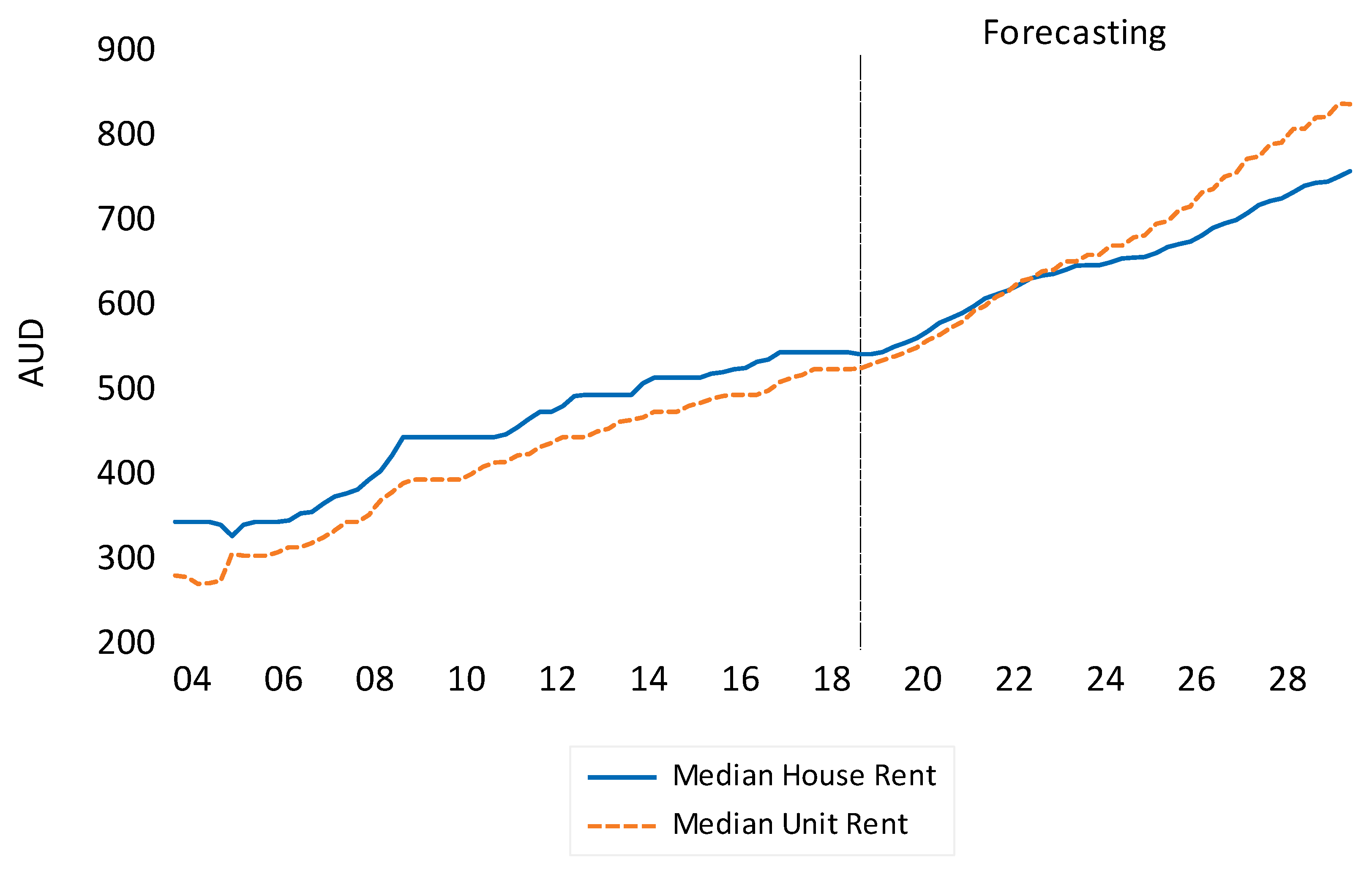
5.4.2. Forecasted Median Rents
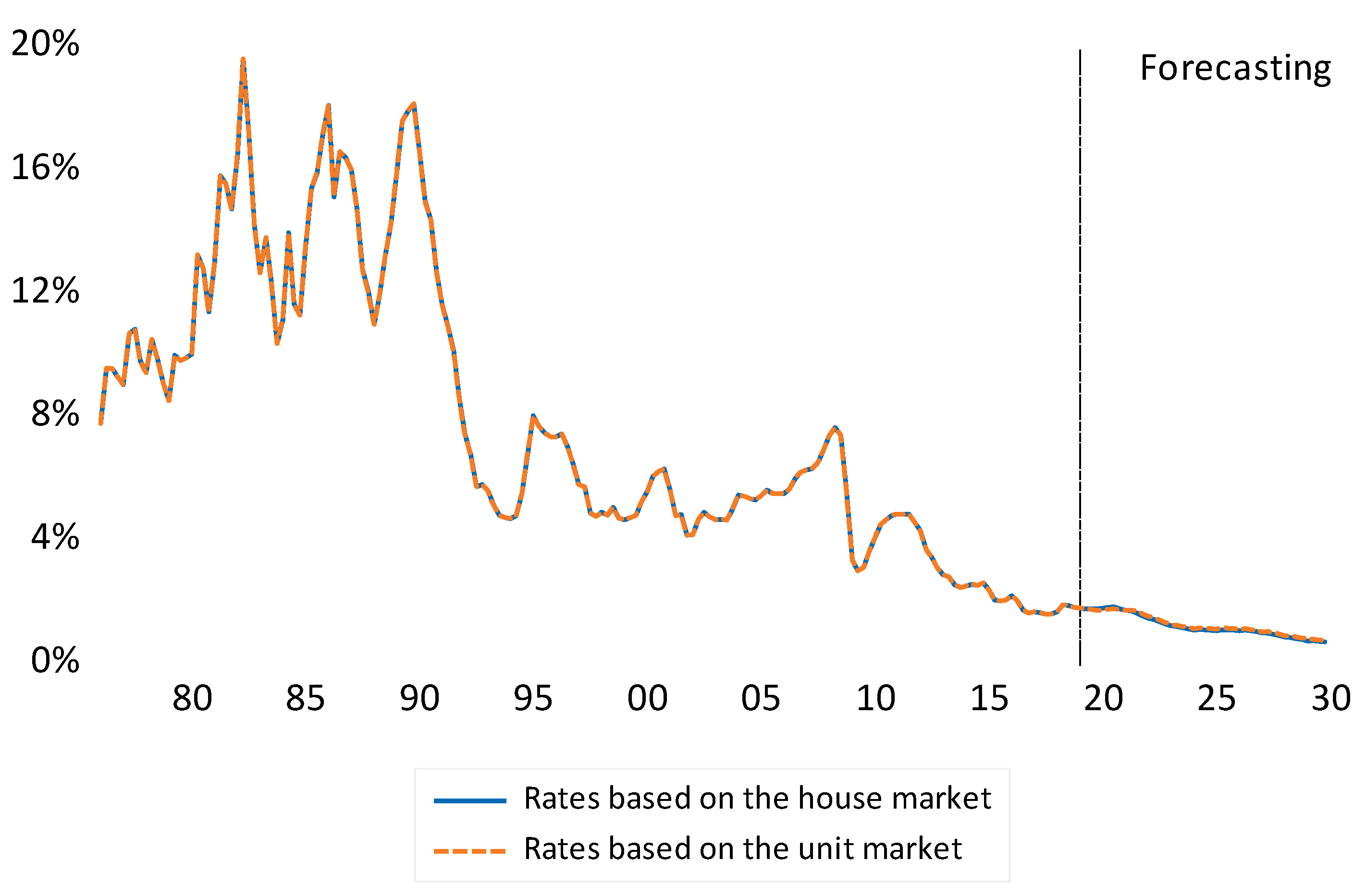
5.4.3. Forecasted Interest Rates
6. Conclusions
Author Contributions
Funding
Acknowledgments
Conflicts of Interest
Appendix A

| (1) | (2) | |
|---|---|---|
| House Price Changes | Unit Price Changes | |
| CointEq1 | −0.084 *** | −0.074 ** |
| (0.025) | (0.030) | |
| D(LOG(SYD_HP_MEDIAN(-1))) | 0.577 *** | 0.674 *** |
| (0.090) | (0.105) | |
| D(LOG(SYD_RENT(-1))) | 0.104 | −0.016 |
| (0.148) | (0.057) | |
| D(LOG(AUS_INT_90D(-1))) | 0.039 | −0.008 |
| (0.033) | (0.021) | |
| Constant | −0.003 | 0.000 |
| (0.005) | (0.004) | |
| D(LOG(AUS_INT_10YRF)) | −0.017 | −0.015 |
| (0.028) | (0.019) | |
| D(LOG(AUS_LEN_DF)) | −0.006 | −0.002 |
| (0.043) | (0.029) | |
| D(LOG(AUS_CONF)) | −0.143 | −0.073 |
| (0.3540) | (0.278) | |
| D(LOG(NSW_PPGF)) | −0.006 | |
| (0.005) | ||
| D(LOG(SYD_SUP_DF)) | 0.011 | −0.000 |
| (0.012) | (0.009) | |
| D(LOG(SYD_NOMF)) | 0.072 | 0.076 ** |
| (0.045) | (0.033) | |
| ECC_PCF | 0.001 * | 0.000 |
| (0.000) | (0.000) | |
| Seasonal dummy | Yes | Yes |
| Adj. R-squared | 0.827 | 0.806 |
| Sum sq. resids | 0.002 | 0.001 |
| S.E. equation | 0.010 | 0.007 |
| F-statistic | 14.650 | 11.954 |
| Log likelihood | 131.030 | 146.459 |
| Akaike AIC | −6.16 | −6.919 |
| Schwarz SC | −5.556 | −6.272 |
| Mean dependent | 0.008 | 0.009 |
| S.D. dependent | 0.023 | 0.015 |
| The cointegration equation results | ||
| LOG(SYD_HP_MEDIAN_H(-1)) | 1.000 | 1.000 |
| LOG(SYD_RENT_H(-1)) | −0.373 (0.202) * | −0.550 (0.079) *** |
| LOG(AUS_INT_90D(-1)) | 0.427 (0.102) *** | 0.280 (0.042) *** |
| Constant | −11.588 | −10.113 |
Appendix B
| Models | obs. | RMSE | MAE | MAPE | Theil |
|---|---|---|---|---|---|
| Panel A: Houses | |||||
| AR(1) | 20 | 84,743 | 74,407 | 8.179 | 0.051 |
| ECM without economic variables | 20 | 91,834 | 78,256 | 9.626 | 0.055 |
| Panel B: Units | |||||
| AR(1) | 20 | 27,524 | 22,353 | 3.256 | 0.021 |
| ECM without economic variables | 20 | 46,490 | 39,064 | 6.140 | 0.036 |
Appendix C

Appendix D

| 1 | A time series process with a unit root (a random walk). |
| 2 | The statistical area of the Greater Sydney Area is maintained by the Australian Bureau of Statistics. For 35 LGAs and their geographic locations and boundaries, please go to the Australian Bureau of Statistics website at: https://dbr.abs.gov.au/index.html (accessed on 25 July 2021). |
| 3 | The authors went through a wide range of data collection in this study. As not all variables are available or statistically significant in our model, we only report the key variables used in the ECM model, as shown in Table 1. Please contact the corresponding author for a complete list of variables collected in this study. |
| 4 | Results of Johansen’s cointegration test are available on request from the corresponding author. |
| 5 | Results are available on request by contacting the corresponding author. |
References
- Malpezzi, S. A simple error correction model of house prices. J. Hous. Econ. 1999, 8, 27–62. [Google Scholar] [CrossRef]
- Francke, M.K.; Vujic, S.; Vos, G.A. Evaluation of House Price Models Using an ECM Approach: The Case of the Netherlands; Methodological Paper No. 2009-05; Ortec Finance Research Center: Rotterdam, The Netherlands, 2009. [Google Scholar]
- Gattini, L.; Hiebert, P. Forecasting and Assessing Euro Area House Prices through the Lens of Key Fundamentals; Working Paper Series No. 1249; European Central Bank: Frankfurt, Germany, 2010. [Google Scholar]
- Shi, S.; Jou, J.B.; Tripe, D. Can interest rates really control house prices? Effectiveness and implications for macro prudential policy. J. Bank. Financ. 2014, 47, 15–28. [Google Scholar]
- Shi, S.; Valadkhani, A.; Smyth, R.; Vahid, F. Dating the timeline of house price bubbles in Australian capital cities. Econ. Rec. 2016, 92, 590–605. [Google Scholar] [CrossRef]
- Wheaton, W.; Chervachidze, S.; Nechayev, G. Error Correction Models of MSA Housing “Supply” Elasticities: Implications for Price Recovery; Working Paper Series No. 07-15; Center for Real Estate, Massachusetts Institute of Technology: Cambridge, MA, USA, 2014. [Google Scholar]
- Yanotti, M.B.; Wright, D. Residential property in Australia: Mismatched investment and rental demand. Hous. Stud. 2021. [Google Scholar] [CrossRef]
- Mankiw, N.G.; Weil, D.N. The baby boom, the baby bust, and the housing market. Reg. Sci. Urban Econ. 1989, 19, 235–258. [Google Scholar] [CrossRef] [Green Version]
- Shiller, R. Long-term perspective on the current boom in home prices. Econ. Voice 2006, 3, 1–11. [Google Scholar] [CrossRef]
- Engsted, T.; Nielsen, B. Testing for rational bubbles in a coexplosive vector autoregression. Econ. J. 2012, 15, 226–254. [Google Scholar] [CrossRef] [Green Version]
- Engsted, T.; Hviid, S.J.; Pedersen, T.Q. Explosive bubbles in house prices? Evidence from the OECD countries. J. Int. Financ. Mark. Inst. Money 2016, 40, 14–25. [Google Scholar] [CrossRef]
- Gyourko, J.; Sinai, T. The spatial distribution of housing-related ordinary income tax benefits. Real Estate Econ. 2003, 31, 527–575. [Google Scholar] [CrossRef] [Green Version]
- Hendershott, P.H.; Slemrod, J. Taxes and the user cost of capital for owner-occupied housing. J. Am. Real Estate Urban Econ. Assoc. 1983, 10, 375–393. [Google Scholar] [CrossRef] [Green Version]
- Himmelberg, C.; Mayer, C.; Sinai, T. Assessing high house prices: Bubbles, fundamentals, and misperceptions. J. Econ. Perspect. 2005, 19, 67–92. [Google Scholar] [CrossRef] [Green Version]
- Meese, R.; Wallace, N. Testing the present value relation for housing prices: Should I leave my house in San Francisco? J. Urban Econ. 1994, 35, 245–266. [Google Scholar] [CrossRef]
- Poterba, J. Tax subsidies to owner-occupied housing: An asset market approach. Q. J. Econ. 1984, 99, 729–752. [Google Scholar] [CrossRef] [Green Version]
- Case, K.E.; Shiller, R.J. The efficiency of the market for single family homes. Am. Econ. Rev. 1989, 79, 125–137. [Google Scholar]
- Bourassa, S.C.; Hoesli, M.; Oikarinen, E. Measuring house price bubbles. Real Estate Econ. 2016, 47, 534–563. [Google Scholar] [CrossRef]
- Campbell, J.Y.; Shiller, R.J. The dividend-price ratio and expectations of future dividends and discount factors. Rev. Financ. Stud. 1988, 1, 195–227. [Google Scholar] [CrossRef] [Green Version]
- Campbell, J.Y.; Shiller, R.J. Stock prices, earnings, and expected dividends. J. Financ. 1988, 43, 661–676. [Google Scholar] [CrossRef]
- Campbell, J.Y.; Shiller, R.J. Cointegration and tests of present value models. J. Political Econ. 1987, 95, 1062–1088. [Google Scholar] [CrossRef] [Green Version]
- Diba, B.T.; Grossman, H.I. Explosive rational bubbles in stock prices? Am. Econ. Rev. 1988, 78, 520–530. [Google Scholar]
- Gallin, J. The long-run relationship between house prices and rents. Real Estate Econ. 2008, 36, 635–658. [Google Scholar] [CrossRef] [Green Version]
- Brooks, C.; Katsaris, A.; McGough, T.; Tsolacos, S. Testing for bubbles in real estate price cycles. J. Prop. Res. 2001, 18, 341–346. [Google Scholar] [CrossRef]
- Stock, J.H.; Watson, M.W. Evidence on structural instability in macroeconomic time series relations. J. Bus. Econ. Stat. 1996, 14, 11–30. [Google Scholar]
- Elliott, G.; Muller, U.K. Confidence sets for the date of a single break in linear time series regressions. J. Econ. 2007, 141, 1196–1218. [Google Scholar] [CrossRef] [Green Version]
- Elliott, G.; Muller, U.K. Pre and post break parameter inference. J. Econ. 2014, 180, 141–157. [Google Scholar] [CrossRef] [Green Version]
- Pesaran, M.H.; Pick, A.; Timmermann, A. Variable selection, estimation and inference for multi-period forecasting problems. J. Econ. 2011, 164, 173–187. [Google Scholar] [CrossRef]
- Renigier-Biłozor, M.; Walacik, M.; Źróbek, S.; d’Amato, M. Forced sale discount on property market–How to assess it? Land Use Policy 2018, 78, 104–115. [Google Scholar] [CrossRef]
- Berry, M.; Dalton, T. Housing prices and policy dilemmas: A peculiarly Australian problem? Urban Policy Res. 2004, 22, 69–91. [Google Scholar] [CrossRef]
- Shi, S.; Kabir, M.H. Catch animal spirits in auction: Evidence from New Zealand property market. Real Estate Econ. 2018, 46, 59–84. [Google Scholar] [CrossRef]
- Commins, P. Lowe Warns Rates Could Stay Low ‘for a Long, Long Time’. The Australian Financial Review. Available online: https://www.afr.com/policy/economy/lowe-warns-rates-could-stay-low-for-a-long-long-time-20190925-p52uun (accessed on 25 September 2019).


| Variable | Definition | Sources |
|---|---|---|
| SYD_HP_MEDIAN_H | Median house prices in the Greater Sydney Area | SIRCA |
| SYD_RENT_H | Median house rents in the Greater Sydney Area | SIRCA |
| SYD_HP_MEDIAN_U | Median unit prices in the Greater Sydney Area | SIRCA |
| SYD_RENT_U | Median unit rents in the Greater Sydney Area | SIRCA |
| AUS_INT_90D | Australia 90-day bill rate | Datastream |
| AUS_INT_10YRF | Australian ten-year government bond yield | Datastream |
| AUS_LEN_DF | Bank mortgage lending for all dwelling finance in Australia | ABS |
| AUS_CONF | Building construction cost index of Australia | ABS |
| NSW_PPGF | New South Wales population growth | ABS |
| SYD_SUP_DF | Total number of dwelling (all types) supply in the Greater Sydney Area | NSW Planning & Environment |
| SYD_NOMF | Net migration numbers in the Greater Sydney Area | ABS |
| ECC_PCF | Residential Property Price Index percentage change from the corresponding quarter of the previous year-weighted average of eight capital cities | ABS |
| Variable Transformation | ||
| D(LOG(SYD_HP_MEDIAN_H)) | Changes in median house prices | |
| D(LOG(SYD_RENT_H)) | Changes in median house rents | |
| D(LOG(SYD_HP_MEDIAN_U)) | Changes in median unit prices | |
| D(LOG(SYD_RENT_U)) | Changes in median unit rents | |
| D(LOG(AUS_LEN_DF)) | Growth rate of bank mortgage lending | |
| D(LOG(AUS_CONF)) | Changes in building construction costs | |
| D(LOG(NSW_PPGF)) | Changes in population growth | |
| D(LOG(SYD_NOMF)) | Changes in net migration numbers |
| (1) | (2) | |
|---|---|---|
| House Price Changes | Unit Price Changes | |
| CointEq1 | −0.048 *** | −0.046 *** |
| (0.014) | (0.015) | |
| D(LOG(SYD_HP_MEDIAN(-1))) | 0.536 *** | 0.639 *** |
| (0.071) | (0.076) | |
| D(LOG(SYD_RENT(-1))) | 0.009 | −0.007 |
| (0.107) | (0.054) | |
| D(LOG(AUS_INT_90D(-1))) | 0.017 | −0.007 |
| (0.021) | (0.014) | |
| Constant | −0.002 | −0.000 |
| (0.003) | (0.003) | |
| D(LOG(AUS_INT_10YRF)) | −0.003 | −0.001 |
| (0.015) | (0.011) | |
| D(LOG(AUS_LEN_DF)) | 0.007 | 0.011 |
| (0.034) | (0.025) | |
| D(LOG(AUS_CONF)) | −0.291 | −0.210 |
| (0.269) | (0.215) | |
| D(LOG(NSW_PPGF)) | −0.003 | |
| (0.004) | ||
| D(LOG(SYD_SUP_DF)) | 0.003 | −0.006 |
| (0.008) | (0.007) | |
| D(LOG(SYD_NOMF)) | 0.042 | 0.052 * |
| (0.036) | (0.028) | |
| ECC_PCF | 0.002 *** | 0.001 *** |
| (0.000) | (0.000) | |
| Seasonal dummy | Yes | Yes |
| Adj. R-squared | 0.843 | 0.812 |
| Sum sq. resids | 0.003 | 0.006 |
| S.E. equation | 0.009 | 0.012 |
| F-statistic | 24.567 | 2.966 |
| Log likelihood | 200.977 | 184.466 |
| Akaike AIC | −6.447 | −5.878 |
| Schwarz SC | −5.95 | −5.38 |
| Mean dependent | 0.012 | 0.008 |
| S.D. dependent | 0.022 | 0.014 |
| The cointegration equation results | ||
| LOG(SYD_HP_MEDIAN_H(-1)) | 1.000 | 1.000 |
| LOG(SYD_RENT_H(-1)) | −0.262 (0.249) | −0.500 (0.117) |
| LOG(AUS_INT_90D(-1)) | 0.582 (0.077) *** | 0.412 (0.043) *** |
| Constant | −12.475 | −10.609 |
| Variable | obs. | RMSE | MAE | MAPE | Theil |
|---|---|---|---|---|---|
| Panel A: Actual | |||||
| Median house prices | 20 | 22,578 | 19,003 | 2.207 | 0.013 |
| Median unit prices | 20 | 31,923 | 23,047 | 3.141 | 0.024 |
| Panel B: Statistical models | |||||
| ARIMA model | |||||
| Median house prices | 20 | 53,771 | 45,449 | 5.368 | 0.032 |
| Median unit prices | 20 | 24,593 | 20,107 | 2.299 | 0.014 |
| AR(1) model | |||||
| Median house prices | 20 | 59,000 | 49,203 | 5.776 | 0.035 |
| Median unit prices | 20 | 18,484 | 14,111 | 2.068 | 0.014 |
| AR(4) model | |||||
| Median house prices | 20 | 70,685 | 59,990 | 7.172 | 0.042 |
| Median unit prices | 20 | 21,640 | 18,154 | 2.729 | 0.016 |
| AR(8) model | |||||
| Median house prices | 20 | 64,694 | 54,936 | 6.534 | 0.038 |
| Median unit prices | 20 | 21,370 | 18,047 | 2.688 | 0.016 |
| AR(16) model | |||||
| Median house prices | 20 | 46,217 | 39,780 | 4.712 | 0.027 |
| Median unit prices | 20 | 25,551 | 19,379 | 2.836 | 0.019 |
| AR(20) model | |||||
| Median house prices | 20 | 37,305 | 31,007 | 3.677 | 0.022 |
| Median unit prices | 20 | 30,753 | 23,981 | 3.397 | 0.023 |
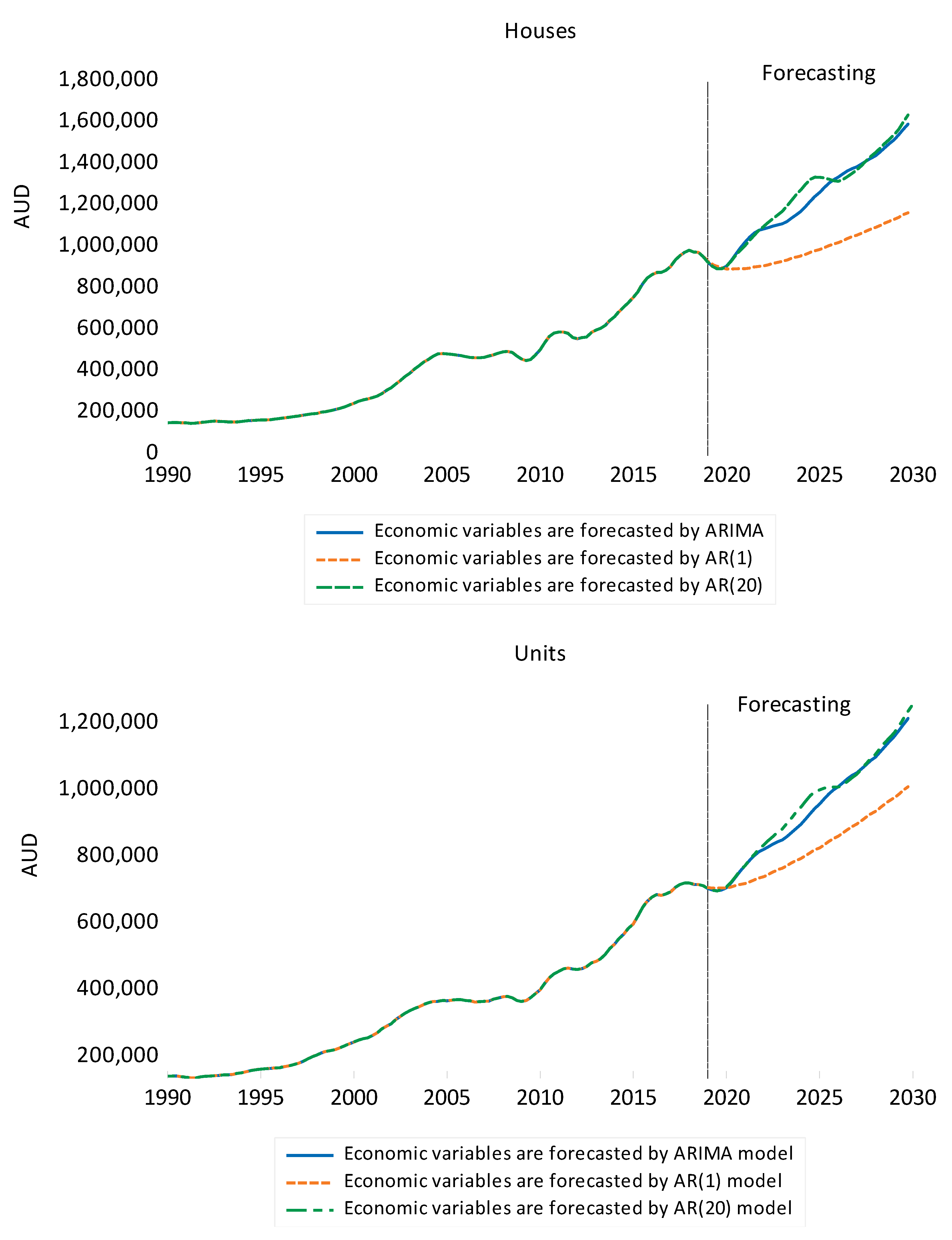
| Houses | Units | |||||
|---|---|---|---|---|---|---|
| Time Period | ARIMA | AR(1) | AR(20) | ARIMA | AR(1) | AR(20) |
| 2019Q1 | 931,067 | 935,696 | 930,709 | 708,278 | 711,058 | 707,385 |
| 2019Q2 | 911,194 | 919,994 | 910,228 | 703,633 | 709,259 | 702,693 |
| 2019Q3 | 899,668 | 910,522 | 898,726 | 701,262 | 709,549 | 701,167 |
| 2019Q4 | 899,592 | 902,946 | 898,575 | 704,042 | 709,965 | 705,222 |
| 2020Q1 | 911,688 | 897,870 | 910,480 | 710,599 | 709,785 | 712,396 |
| 2020Q2 | 937,604 | 896,699 | 935,054 | 725,269 | 712,940 | 727,899 |
| 2020Q3 | 969,586 | 898,580 | 963,080 | 742,813 | 717,425 | 744,982 |
| 2020Q4 | 1,000,454 | 899,203 | 988,440 | 761,172 | 721,061 | 762,201 |
| 2021Q1 | 1,026,564 | 899,777 | 1,010,434 | 776,647 | 723,352 | 776,808 |
| 2021Q2 | 1,051,763 | 902,546 | 1,035,673 | 793,422 | 728,505 | 794,303 |
| 2021Q3 | 1,072,154 | 907,377 | 1,061,955 | 807,664 | 734,725 | 810,899 |
| 2021Q4 | 1,084,812 | 910,416 | 1,085,048 | 818,901 | 739,903 | 827,012 |
| 2022Q1 | 1,090,764 | 913,157 | 1,103,916 | 825,515 | 743,606 | 838,728 |
| 2022Q2 | 1,097,922 | 918,003 | 1,122,849 | 833,694 | 750,172 | 852,274 |
| 2022Q3 | 1,104,906 | 924,863 | 1,141,454 | 841,290 | 757,768 | 864,616 |
| 2022Q4 | 1,110,291 | 929,794 | 1,158,450 | 848,505 | 764,205 | 877,111 |
| 2023Q1 | 1,115,409 | 934,287 | 1,176,081 | 854,240 | 769,020 | 887,132 |
| 2023Q2 | 1,127,265 | 940,781 | 1,201,009 | 864,403 | 776,693 | 902,642 |
| 2023Q3 | 1,143,098 | 949,182 | 1,229,239 | 876,219 | 785,338 | 919,601 |
| 2023Q4 | 1,159,630 | 955,449 | 1,255,977 | 888,902 | 792,691 | 937,265 |
| 2024Q1 | 1,176,506 | 961,117 | 1,280,240 | 900,605 | 798,278 | 951,949 |
| 2024Q2 | 1,199,588 | 968,711 | 1,307,132 | 916,464 | 806,760 | 970,516 |
| 2024Q3 | 1,224,766 | 978,157 | 1,329,884 | 933,008 | 816,191 | 986,871 |
| 2024Q4 | 1,247,488 | 985,306 | 1,341,254 | 948,795 | 824,226 | 999,107 |
| 2025Q1 | 1,267,094 | 991,752 | 1,340,653 | 961,684 | 830,379 | 1,003,737 |
| 2025Q2 | 1,289,900 | 1,000,113 | 1,336,449 | 977,148 | 839,503 | 1,009,010 |
| 2025Q3 | 1,311,892 | 1,010,324 | 1,330,797 | 991,885 | 849,581 | 1,011,236 |
| 2025Q4 | 1,328,916 | 1,018,109 | 1,324,326 | 1,004,629 | 858,177 | 1,012,546 |
| 2026Q1 | 1,341,300 | 1,025,120 | 1,321,241 | 1,013,773 | 864,786 | 1,012,437 |
| 2026Q2 | 1,356,635 | 1,034,069 | 1,329,277 | 1,025,616 | 874,466 | 1,019,592 |
| 2026Q3 | 1,371,711 | 1,044,895 | 1,343,665 | 1,037,221 | 885,119 | 1,029,243 |
| 2026Q4 | 1,382,851 | 1,053,181 | 1,359,345 | 1,047,595 | 894,211 | 1,040,725 |
| 2027Q1 | 1,390,980 | 1,060,639 | 1,374,828 | 1,055,374 | 901,217 | 1,050,439 |
| 2027Q2 | 1,404,237 | 1,070,076 | 1,396,359 | 1,067,094 | 911,409 | 1,066,013 |
| 2027Q3 | 1,419,395 | 1,081,436 | 1,420,529 | 1,079,755 | 922,604 | 1,082,358 |
| 2027Q4 | 1,432,427 | 1,090,149 | 1,441,346 | 1,092,156 | 932,161 | 1,098,464 |
| 2028Q1 | 1,444,141 | 1,097,988 | 1,459,068 | 1,102,630 | 939,534 | 1,110,928 |
| 2028Q2 | 1,462,484 | 1,107,862 | 1,480,598 | 1,117,673 | 950,221 | 1,128,060 |
| 2028Q3 | 1,483,687 | 1,119,714 | 1,503,627 | 1,133,929 | 961,946 | 1,144,919 |
| 2028Q4 | 1,503,083 | 1,128,815 | 1,524,299 | 1,149,803 | 971,957 | 1,161,090 |
| 2029Q1 | 1,521,148 | 1,137,001 | 1,544,480 | 1,163,369 | 979,686 | 1,174,553 |
| 2029Q2 | 1,545,758 | 1,147,287 | 1,572,678 | 1,181,283 | 990,865 | 1,194,720 |
| 2029Q3 | 1,572,689 | 1,159,614 | 1,606,490 | 1,199,862 | 1,003,123 | 1,216,369 |
| 2029Q4 | 1,596,568 | 1,169,086 | 1,640,703 | 1,217,315 | 1,013,591 | 1,238,525 |
Publisher’s Note: MDPI stays neutral with regard to jurisdictional claims in published maps and institutional affiliations. |
© 2021 by the authors. Licensee MDPI, Basel, Switzerland. This article is an open access article distributed under the terms and conditions of the Creative Commons Attribution (CC BY) license (https://creativecommons.org/licenses/by/4.0/).
Share and Cite
Shi, S.; Mangioni, V.; Ge, X.J.; Herath, S.; Rabhi, F.; Ouysse, R. House Price Forecasting from Investment Perspectives. Land 2021, 10, 1009. https://doi.org/10.3390/land10101009
Shi S, Mangioni V, Ge XJ, Herath S, Rabhi F, Ouysse R. House Price Forecasting from Investment Perspectives. Land. 2021; 10(10):1009. https://doi.org/10.3390/land10101009
Chicago/Turabian StyleShi, Song, Vince Mangioni, Xin Janet Ge, Shanaka Herath, Fethi Rabhi, and Rachida Ouysse. 2021. "House Price Forecasting from Investment Perspectives" Land 10, no. 10: 1009. https://doi.org/10.3390/land10101009
APA StyleShi, S., Mangioni, V., Ge, X. J., Herath, S., Rabhi, F., & Ouysse, R. (2021). House Price Forecasting from Investment Perspectives. Land, 10(10), 1009. https://doi.org/10.3390/land10101009