Nonlinear Influence of Public Services on Urban Housing Prices: A Case Study of China

Abstract

Owing to China’s rapid urbanization and internal migration, public services are unevenly distributed in cities, affecting urban housing prices. This study examines the dynamic effect of China’s public service levels on urban housing prices. We used the entropy method to calculate the public service index of 30 cities in China and a panel threshold regression model to explore the relationship between urban public service levels and housing prices. We found that the degree of the effect of public service levels on urban housing prices varies with the per capita disposable income of urban residents, demonstrating an inverted U-shaped curve. The role of public services in promoting urban housing prices increases with the increase in the level of urbanization. When the level of urbanization exceeds its threshold, the enhancement effect increases. These results help us better understand the theories of housing price changes in Chinese cities and support policymakers in formulating effective control measures for the housing market.

1. Introduction

Public services refer to the basic products and services related to the survival and development of residents, such as compulsory education, basic medical care, public infrastructure, and environment sanitation [1]. These services not only meet the characteristics of publicity but also require the participation of the government. Several studies have found that urban public services have significant externalities, which can increase the satisfaction and happiness of residents, attract the flow of urban population, and gradually become an important factor in determining residents’ quality of life [2,3,4]. Therefore, the distribution pattern of public service facilities promotes the formation and evolution of urban housing prices by influencing residents’ house purchase intentions. At the macro level, this distribution is not only a market response to the unbalanced allocation of urban space resources but also an important mechanism for promoting the separation of social space [5]. Moreover, the level of public services in different cities is also different. The mismatch of housing supply and demand has resulted in soaring housing prices in advantageous cities. The premium effect of public service levels in the housing market further promotes competition among different social groups and exacerbates spatial inequality in China’s housing market. Achieving equalization of public service levels plays a very important role in coordinating the coordinated development of urban and rural areas and regions.

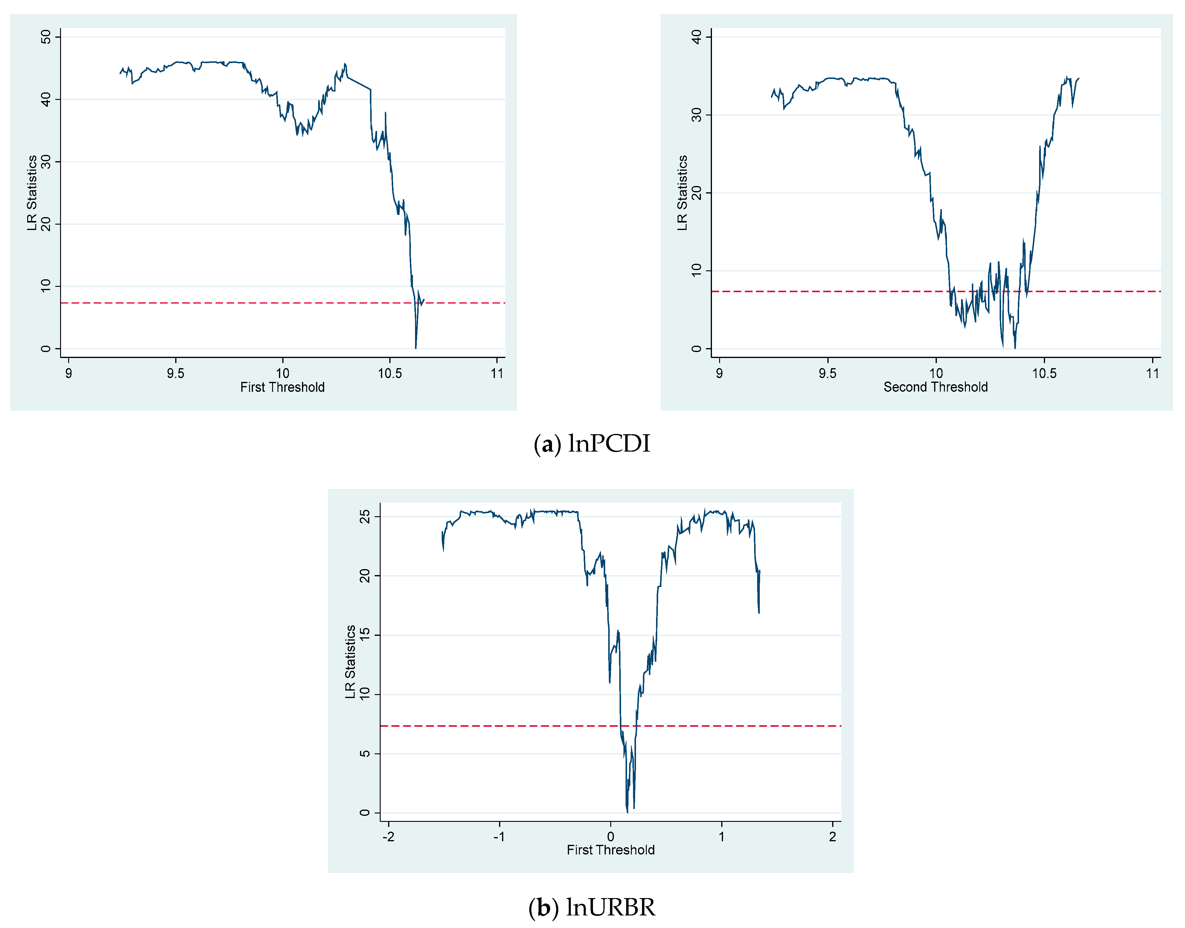
Existing studies have also explored the relationship between various public service levels and urban housing prices, but there is no consensus on the key factors affecting housing price differences in different regions. These works are mainly based on traditional characteristic price models, spatial regression models, and geographically weighted regression models. These models are limited to analyzing the significance and direction of the effect of certain types of facilities on housing prices. However, there are many factors affecting the development of China’s real estate market, and the influencing parameters of real estate prices are not stable. As shown in Figure 1, China’s public service level has a non-linear effect on urban real estate prices. At this time, the linear relationship between variables may not be able to reveal the law of real estate price fluctuations and their influencing factors. From a non-linear perspective, we can become richer and obtain more in-depth conclusions by discussing the volatility of public services on housing prices in Chinese cities.

Based on previous research on China’s public service level [6,7,8], we identified four types of public service facilities, namely education, medical care, environmental, and transportation services, to represent the level of public service in China. By using threshold regression models and by analyzing the difference between public service levels and residential prices in 30 large and medium-sized cities in China, we further explore the dynamic influence path of different regional public service levels on real estate price changes.

This study fills the following gap in the literature. First, we employ the threshold regression model in order to reveal the dynamic effect of China’s public service levels on housing prices based on the difference in housing prices among cities in resource allocation. Second, considering the heterogeneity of urban public service levels, we study the effect of public services on real estate prices by region and analyze the reasons thereof. Third, the literature generally uses official statistics of population urbanization rate indicators, which have certain drawbacks. The urbanization indicators obtained by processing night light data in this study have higher credibility.

The remainder of this paper is structured as follows: Section 2 reviews the body of academic research on public services and the related literature on the effects of public services on housing prices. Section 3 elaborates on the empirical methods employed and the data sources. Section 4 shows the empirical results. Section 5 discusses the results. Finally, the conclusions and related policy recommendations are presented in Section 6.

2. Literature Review

In 1912, the French public jurist Leon Duguit conceived the concept of public service: “An activity is a public service, as long as it has the characteristics that it cannot be guaranteed unless it is through government intervention” [9]. Eleanor Ostrom proposed the concept of “public pond resources” and discussed the possibility of autonomous management of “public ponds” [10], which further enriched public service theory. Further studies on public services have also contributed to envisioning a perfect theoretical system of public service and guided subsequent research on the topic [11,12,13].

American economist Tiebout [14], for example, put forward the theory of “voting with feet” in the field of public service products in 1956. Among them, the research on the spillover effects of public services has really begun to attract scholarly attention. This theory mainly studies consumers’ preference in the selection of public service products and the efficiency of public service products, which allows one to expand and empirically analyze the problem from multiple angles. In this regard, the focus is mainly on public service facilities that are closely related to residents’ lives, such as the environment, education, transportation, and medical care.

In terms of the environment, Zhang et al. [15] claimed that air pollution has a spillover effect on local housing prices, while Dai et al. [16] noted that areas with higher environmental risks, such as gas stations and chemical companies, have lower housing prices, and different risks result in an inverted U-shaped relationship between housing prices and total environmental risks. Chen and Li [17] confirmed that cities close to polluted rivers significantly reduce apartment prices, and buyers are willing to pay an additional premium for apartments far away from the two polluted rivers.

In terms of educational facilities, Han et al. [18] found that the average educational premium of high-quality primary schools to housing prices is about 11%, and it is increasing every year. Wen et al. [19] showed that the effect of educational facilities on housing prices is quite different; primary and secondary schools have significantly higher housing prices, while kindergartens are only valued by buyers of low and high housing prices. Wen et al. [20] believed that educational facilities have a positive capitalization effect on housing prices, and elementary and junior high schools have significant school district effects.

In terms of transportation, Yang et al. [21] noted that the premium and negative effects of public transportation on housing prices exist at the same time and they are spatially heterogeneous. Buyers of high housing prices are willing to pay more for staying away from public transportation. Tsai [22] holds that improving transportation infrastructure can shorten the invisible distance among cities, promote interaction among cities, and promote the convergence of housing prices. Dai et al. [23] showed that both the transfer station and non-transfer station of Beijing rail transit have a value-added effect on the price of surrounding houses, but the increase with respect to the transfer station is even greater.

In terms of medical care, Wang et al.’s [24] research on several megacities in China finds that hospitals near communities are positively correlated with housing values; the farther away from the hospital, the lower the value of the house [25].

While public services benefit urban housing prices, this relationship is not certain in all countries around the world. For example, ordinary housing has a significantly positive effect on the prices of transportation hubs, central business district, medical service center, and school district, while expensive houses do not [26]. Andersson et al. [27] estimated the implied price of Tainan’s urban high-speed rail and found that its effect on housing prices is marginal and even negligible. Pang and Jiao [28] found that the effect of Metro Line 3 on property prices around Beijing is also negligible. Wen et al. [29] showed that public transportation in Hangzhou City cannot increase the value-added effect of houses. Wen et al. [20] and Wen and Tao [30] also confirmed that the accessibility of buses harms the real estate value of Hangzhou. In addition, the influence of the degree of public services or infrastructure in many developed regions on housing prices is not so significant. For example, proximity to bus stops, train stations, or highways has no significant impact on the value of housing in rural areas in Northeastern Slovenia. Moreover, the proximity of railway tracks is significantly negatively correlated with price [31]. The sizes of the houses and the distance from the city center have a greater impact on housing prices in Seoul, South Korea, than its transportation convenience [32]. The negative impact of the transportation system on housing prices in Utah is even greater than the positive impact [33]. The location and neighborhood characteristics of the house will not have a significant impact on the price of the house [34].

Therefore, the conclusion that the degree of public services has a positive influence on urban housing prices cannot be applied to all regions. As Epple et al. [35] stated, the Tiebout model only confirms that differences in public services between regions will cause relative housing prices to rise, but it cannot explain the specific relationship between public services and the overall housing price level. Thus, some strict assumptions in Tiebout’s theory may not be completely correct, but research does confirm a certain Tiebout effect in China, that is, the supply of local public goods has a certain effect on housing prices.

In short, we can see that the externalities of China’s public service level can produce positive, marginal (insignificant), or negative externalities toward neighboring real estate. There is still no unified conclusion. There are still a few studies on the dynamic effect of public service levels on housing prices. To make up for these research gaps, it is noteworthy to study the influence of China’s public service level on urban housing prices.

3. Methods and Data

3.1. Panel Threshold Model

The threshold analysis method is one of the important methods for studying the nonlinear relationship among variables. The traditional method is often conducted by simply dividing the section, and the selection of segmentation points is usually given exogenously, and the threshold is selected subjectively. It is not determined by the internal mechanism of the economic system, which weakens the validity of the parameter estimation obtained by this threshold segmentation method. In response to this problem, Hensen [36] proposed a new panel threshold regression method. This method does not requiring setting the non-linear equation form in advance; the threshold value and its number are determined endogenously by sample data, thus avoiding exogeneity, which is suitable for studying real estate prices with complex influencing factors. The basic form of the panel threshold regression model is the following:

$${\mathrm{y}}_{\mathrm{it}}={ \mathsf{\mu }}_{\mathrm{i}}+{ \mathrm{x}}_{\mathrm{it}}{\mathsf{\beta }}_1\mathrm{I} \left({\mathrm{q}}_{\mathrm{it}} \le \mathsf{\gamma }\right)+{ \mathrm{x}}_{\mathrm{it}}{\mathsf{\beta }}_2\mathrm{I} \left({\mathrm{q}}_{\mathrm{it}}> \mathsf{\gamma }\right)+{ \mathsf{\epsilon }}_{\mathrm{it}}$$

(1)

where $\mathrm{i} =1, 2,\cdots , \mathrm{N}$ denotes the individuals, $\mathrm{t} =1, 2, \dots , \mathrm{T}$denotes time, $\mathrm{I} \{• \}$ is an indicator function, and ${\mathsf{\epsilon }}_{\mathrm{it}}$ is subject to independent and identical distribution with a mean value of 0 and a variance of ${\mathsf{\sigma }}_{\mathsf{\epsilon }}{}^2$. ${\mathrm{q}}_{\mathrm{it}}$ is the “threshold variable”; it can be either the explanatory variables or an independent variable. According to its corresponding “threshold value” $\mathsf{\gamma }$, all samples can be divided into two intervals, and the difference between these two intervals is manifested in the regression coefficients, ${\mathsf{\beta }}_1$ and ${\mathsf{\beta }}_2$. After removing the average within the group, the conditional least squares method can be used to obtain the consistent estimator of the parameter $\mathsf{\beta }$. If the corresponding residual sum of squares is recorded as ${\mathrm{S}}_{\mathrm{n}}\left(\mathsf{\gamma }\right)$, then the estimated value of the threshold $\mathsf{\gamma }$ can be obtained by $\hat{\mathsf{\gamma }}={ \mathrm{argminS}}_{\mathrm{n}}\left(\mathsf{\gamma }\right)$.

In practice, the model may also have two or more thresholds; thus, this process needs to be repeated in order to find other possible thresholds. For example, the model of the two thresholds is the following:

$${\mathrm{y}}_{\mathrm{it}}={ \mathsf{\mu }}_{\mathrm{it}}+{ \mathrm{x}}_{\mathrm{it}}{\mathsf{\beta }}_1\mathrm{I} \left({\mathrm{q}}_{\mathrm{it}} \le { \mathsf{\gamma }}_1\right)+{\mathrm{x}}_{\mathrm{it}}{\mathsf{\beta }}_2\mathrm{I} \left({\mathsf{\gamma }}_1<{ \mathrm{q}}_{\mathrm{it}} \le { \mathsf{\gamma }}_2\right)+{ \mathrm{x}}_{\mathrm{it}}{\mathsf{\beta }}_3\mathrm{I} \left({\mathrm{q}}_{\mathrm{it}}>{ \mathsf{\gamma }}_2\right)+{ \mathsf{\epsilon }}_{\mathrm{it}}$$

(2)

and among them ${\mathsf{\gamma }}_1<{ \mathsf{\gamma }}_2$. First, we assume that the previously estimated threshold value ${\hat{\mathsf{\gamma }}}_1$ is known, and then we use a similar method to obtain the second threshold estimate ${\mathsf{\gamma }}_2$ that minimizes the residual sum of squares. After the second threshold estimate ${\hat{\mathsf{\gamma }}}_2$ is obtained, the threshold effect correlation test is performed again. At this time, the original hypothesis ${\mathrm{H}}_0$ is proposed, that is, there is only one threshold; the alternate hypothesis ${\mathrm{H}}_1$ states that there are two thresholds [37]. The Lagrange multiplier test statistic is the following:

$${\mathrm{F}}_2\left(\mathsf{\gamma }\right)=\frac{{\mathrm{S}}_1\left({\hat{\mathsf{\gamma }}}_1\right)-{ \mathrm{S}}_2\left({\hat{\mathsf{\gamma }}}_2\right)}{{\hat{\mathsf{\sigma }}}_2{}^2}$$

(3)

where ${\mathsf{\sigma }}_2{}^2$ is the residual variance of the second threshold. As the existence of the first threshold was assumed in advance when estimating the second threshold, the estimated result can meet that consistency. However, the consistency is not satisfied when the first threshold is estimated. In order to improve the first threshold value, it needs to be verified again. The specific method is to treat ${\hat{\mathsf{\gamma }}}_2$ as a known threshold, to find another threshold ${\mathsf{\gamma }}_1{}^{*}$ that minimizes the residual sum of squares, and to record the corresponding residual sum of squares as follows.

$${\mathrm{S}}_1{}^{*}\left({\mathsf{\gamma }}_1\right)=\{\begin{array}{c}{\mathrm{S}}_1\left({\mathsf{\gamma }}_1,{\mathsf{\gamma }}_2*\right)\left({\mathsf{\gamma }}_1\le {\mathsf{\gamma }}_2*\right)\\ {\mathrm{S}}_1\left({\mathsf{\gamma }}_1*,{\mathsf{\gamma }}_2\right)({\mathsf{\gamma }}_1>{\mathsf{\gamma }}_2*)\end{array}$$

(4)

The re-estimated threshold is the following.

$${\hat{\mathsf{\gamma }}}_1{}^{*}={ \mathrm{argminS} \mathrm{S}}_1{}^{*}\left({\mathsf{\gamma }}_1\right)$$

(5)

Combined with Hansen’s introduction, this study establishes a threshold panel model of the nonlinear influence of basic public services on urban housing prices:

$$\ln {\mathrm{price}}_{\mathrm{it}}={ \mathsf{\mu }}_{\mathrm{i}}+{ \mathsf{\beta }}_1\ln {\mathrm{pus}}_{\mathrm{it}}+{ \mathsf{\beta }}_2\ln {\mathrm{x}}_{\mathrm{it}}+{ \mathsf{\beta }}_3\ln {\mathrm{pus}}_{\mathrm{it}}\mathrm{I} \left({\mathrm{q}}_{\mathrm{it}} \le \mathsf{\gamma }\right)+{\mathsf{\beta }}_4\ln {\mathrm{pus}}_{\mathrm{it}}\mathrm{I} \left({\mathrm{q}}_{\mathrm{it}}> \mathsf{\gamma }\right)+{ \mathsf{\epsilon }}_{\mathrm{it}}$$

(6)

where ${\mathrm{price}}_{\mathrm{it}}$ is the housing price level of city $\mathrm{i}$ at time $\mathrm{t}$, while ${\mathrm{pus}}_{\mathrm{it}}$ is the public service level of city $\mathrm{i}$ at time $\mathrm{t}$. Since housing prices are closely related to factors such as the level of urban economic development and population density in order to control the effect of these factors on housing prices, we selected ${\mathrm{x}}_{\mathrm{it}}$ as the control variable in the empirical analysis.

3.2. Variable Selection and Data Sources

We selected 30 cities in China from 2005 to 2018 to build the data set. The selected cities are all sub-provincial cities and above cities (including four municipalities directly under the Central Government, twenty-five provincial capital cities, and one sub-provincial city). In addition, among the provincial capitals, except for Lhasa, Hohhot, and Taipei owing to incomplete statistical data, all other provincial capitals are included. We believe that the 30 large and medium-sized cities in the sample can identify regional differences in the relationship between China’s public services and the housing market, and they are representative. The explained variable is the price of urban real estate, the level of public services is the core explanatory variable, and the threshold variables are the per capita disposable income of urban residents and the level of urbanization. The remaining variables are the control variables. The data are taken from the China City Statistical Yearbook and the National Bureau of Statistics.

Table 1. Descriptive statistics of key variables.

Variable	Mean	SD	Min	Median	Max
price	7838	6182	1870	6337	54,132
pus	0.0100	0	0	0.0100	0.0300
pcdi	26,315	12,125	8397	25,190	67,990
urbr	1.930	2.550	0.0800	1.090	15.17
pgdp	63,223	39,147	10,982	57,467	470,000
inve	638.1	561.2	14.91	462.2	3013
pod	2.120	0.920	0.650	1.960	5.600

shows the descriptive statistical analysis of the relevant variables, and they are described below:

• Urban real estate prices ($\mathrm{PRICE}$): The average selling price of residential commercial houses in each city is used to represent the level of housing prices.
• Public service level ($\mathrm{PUS}$): Based on the literature on the level of public services in China [6,7,8], we comprehensively selected four indicators, namely environmental development, medical level, education level, and traffic level, and used the entropy method to calculate the public service level of China’s 30 large and medium-sized cities from 2005 to 2018. Specifically, environmental development includes urban green area and air quality. The medical level includes the number of beds per 10,000 people and the number of doctors. The education level includes the number of full-time teachers per 10,000 primary and secondary school students and the number of primary and secondary schools. The traffic level includes the number of buses per 10,000 people and the road area per capita. Figure 2 shows the public service levels of 30 cities in China in 2005, 2010, and 2018. With the development of China’s urbanization, more rural people have poured into cities, and people’s demand for energy has increased, resulting in declines in urban air quality and the level of urban public environmental development. In addition, the concentration of population has accelerated the speed of urban renewal, and the per capita road area and the number of buses per 10,000 people have decreased, reducing the development level of urban public transportation. Therefore, we can also find that the degree of public services in some provinces with better economic development has declined in recent years.
• Per capita disposable income ($\mathrm{PCDI}$): We use the per capita disposable income of urban residents in each city in that year. The per capita disposable income refers to the average value of individual disposable income. Personal disposable income is considered to be the most important determinant of consumer spending, and it is often used to measure changes in the living standards of a country or region.
• Urbanization level ($\mathrm{URBR}$): We measure the level of urbanization by vectorizing the night light data. The data can be obtained from Chen et al. [38]. We calculated the composite index of lighting from two aspects: the depth of urban intensive development and the extent of scale expansion. The calculation formula of the light composite index is ${\mathrm{urbr}}_{\mathrm{i}}={ \mathsf{\omega }\mathrm{urbr}}_1{}_{\mathrm{i}}+\left(1- \mathsf{\omega }\right){\mathrm{urbr}}_{2\mathrm{i}}$, where ${\mathrm{urbr}}_{1\mathrm{i}}$ is the urbanization depth measured by the average light intensity; ${\mathrm{urbr}}_{2\mathrm{i}}$ is the extent of urbanization measured by the lighting attributes of the area; and $\mathsf{\omega }\in \left(0,1\right)$ represents the weight of ${\mathrm{urbr}}_{1\mathrm{i}}$. Due to limited space, only the three-year urbanization level is selected, as shown in Figure 3.

• Per capita GDP ($\mathrm{PGDP}$): Per capita GDP is often selected to indicate the level of economic development of a country or region.
• Real estate investment ($\mathrm{INVE}$): We used the amount of residential investment in real estate development to represent the investment cost required for residential commercial housing projects.
• Population density ($\mathrm{POD}$): The ratio of the total population to the built-up area is a key variable for evaluating the current status of regional population distribution.

4. Results

4.1. Data Stationarity Test

4.1.1. Unit Root Test

In order to avoid spurious regression, we first performed a stationarity test on the sample data, which is the panel unit root test. In

Table 2. Panel unit root test results of the variables.

Variable	LLC	IPS	Fisher-ADF
lnPRICE	−5.7270 ***	−4.4197 ***	11.5814 ***
lnPUS	−8.0363 ***	−5.0923 ***	13.1484 ***
lnURBR	−8.0144 ***	−8.1322 ***	8.8063 ***
lnPGDP	−3.2533 ***	−3.1984 ***	8.1887 ***
lnPCDI	−11.7809 ***	−2.6237 ***	11.9504 ***
lnPOD	−1.6617 **	−1.7716 **	10.1073 ***
lnINVE	−4.6908 ***	−1.7199 **	9.0457 ***

Note. The significance levels are at 1% and 5%, and they are represented by *** and **, respectively.

, we find that the test results of the variables under the three methods are all significant, indicating that all variables of the model are stable.

4.1.2. Cointegration Test

According to the results of the unit root test, we found the stationarity of each variable level. Thus, we employed the panel cointegration test to further test whether each variable has long-term equilibrium. The Kao co-integration and the Pedroni co-integration tests are used to verify if such a relationship exists. In

Table 3. Results of the cointegration test of key variables.

Test Statistics	Statistic	Test Statistics	Statistic
Modified Dickey–Fuller t	−0.7664	Modified Phillips–Perron t	8.9891 ***
Dickey–Fuller t	−1.6610 **	Phillips–Perron t	−7.2849 ***
Augmented Dickey–Fuller t	−0.9927 *	Augmented Dickey–Fuller t	−5.9677 ***
Unadjusted modified Dickey–Fuller t	−3.8608 ***	Variance ratio	3.6270 ***
Unadjusted Dickey–Fuller t	−3.4584 ***

Note. The significance levels are at 1%, 5%, and 10% and are represented by ***, **, and *, respectively.

, we can find the results of the cointegration test for each variable.

Table 3 shows that the $\mathrm{t}$ statistics of each variable is significant at all levels, indicating that the variable rejects the null hypothesis of non-cointegration. Therefore, every variable shown in Table 1 is cointegrated, indicating a long-term equilibrium relationship among these variables.

4.2. Threshold Effect Test and Estimation

4.2.1. Threshold Effect Test

By selecting the per capita disposable income of urban residents and the level of urbanization as threshold variables, we derived the results of the threshold effect test of the model. In

Table 4. Test of the threshold effect.

Threshold Variable	Threshold	F Stat	10%	5%	1%	Threshold Value	95% Confidence Interval
lnPCDI	Single	67.94 ***	22.1270	28.4175	35.3812	10.6207	(10.6175,10.6300)
	Double	35.35 ***	16.2840	19.9682	26.0353	10.3647	(10.3468,10.3684)
	Triple	23.66	24.8942	28.6289	35.4057	10.0664	(10.0411,10.0691)
	Single	25.84 **	20.6322	24.6020	36.7797	0.1513	(0.1176,0.1526)
lnURBR	Double	6.21	18.1600	21.1272	30.4918	1.3347	(1.3262,1.3369)
	Triple	5.46	15.8898	20.0175	26.3431	−1.5076	(−1.5147,1.5030)

Note. The significance levels are at 1% and 5%, and they are represented by *** and **, respectively.

, we found that both the single-threshold and the double-threshold tests of per capita disposable income are significant at the 1% level. The single threshold test under the urbanization level is significant at the 5% level. The single and double thresholds of per capita disposable income are RMB 10.6207 and RMB 10.3647, respectively. After removing the logarithmic function of the threshold, the threshold of this indicator is RMB 40,974.29 and RMB 31,719.92, respectively. The single threshold of the urbanization level is 0.1513, and the single threshold after removing the logarithm is 1.1633.

To clearly show the threshold estimation and likelihood-ratio test results under different settings, we drew a graph of the likelihood ratio function. Figure 4 show that when the per capita disposable income of urban residents and the level of urbanization are used as threshold variables, the threshold effect of urban public service levels on real estate prices is significant.

4.2.2. Threshold Model Estimation

We now estimate the threshold effect model with per capita disposable income and urbanization level as threshold variables. The results show that, in the two threshold variable models, the effect of public service levels on urban real estate prices is significant. The estimation results of the threshold model are shown in

Table 5. Threshold regression results with PCDI level as the threshold variable.

Variable	Model 1	Model 2	Model 3	Model 4	Model 5
lnpus(pcdi ≤ γ1)	0.341 ***	0.218 ***	0.0380	0.00700	0.0180
	(0.06)	(0.06)	(0.05)	(0.04)	(0.04)
lnpus(γ1 < pcdi ≤ γ2)	0.228 ***	0.125 *	−0.00300	−0.0170	−0.00900
	(0.06)	(0.07)	(0.05)	(0.04)	(0.04)
lnpus(pcdi > γ2)	0.135 **	0.0360	−0.0640	−0.0630	−0.0470
	(0.06)	(0.06)	(0.05)	(0.04)	(0.04)
lnpod		−0.338 ***	−0.00400	0.170 **	0.103
		(0.09)	(0.07)	(0.07)	(0.07)
lninve			0.406 ***	0.231 ***	0.247 ***
			(0.02)	(0.03)	(0.03)
lnpgdp				0.427 ***	0.497 ***
				(0.05)	(0.05)
lnurbr					−0.109 ***
					(0.03)
cons	9.913 ***	9.543 ***	6.374 ***	2.566 ***	1.842 ***
	(0.29)	(0.29)	(0.26)	(0.50)	(0.47)
N	420	420	420	420	420
r2	0.736	0.758	0.874	0.895	0.899
r2 a	0.715	0.737	0.862	0.885	0.890
F	360.4	301.8	532.4	543.8	489.5

Note. Standard errors in parentheses. * p < 0.1; ** p < 0.05; ***p < 0.01.

and

Table 6. Threshold egression results with URBR as the threshold variable.

Variable	Model 1	Model 2	Model 3	Model 4	Model 5
lnpus(urbr ≤ λ1)	0.667 ***	0.0240	−0.00100	−0.0400	0.0550
	(0.09)	(0.05)	(0.05)	(0.05)	(0.04)
lnpus(urbr > λ1)	0.549 ***	0.00200	−0.0210	−0.0210	0.078 **
	(0.10)	(0.05)	(0.05)	(0.05)	(0.04)
lninve		0.522 ***	0.505 ***	0.221 ***	0.110 ***
		(0.02)	(0.02)	(0.03)	(0.03)
lnpod			−0.112	0.149 **	0.198 ***
			(0.08)	(0.07)	(0.06)
lnpgdp				0.618 ***	0.0880
				(0.05)	(0.05)
lnpcdi					0.773 ***
					(0.06)
cons	11.577 ***	5.678 ***	5.741 ***	0.458	−0.457
	(0.46)	(0.29)	(0.29)	(0.48)	(0.40)
N	420	420	420	420	420
r2	0.330	0.828	0.829	0.877	0.918
r2 a	0.277	0.813	0.814	0.866	0.911
F	95.76	619.2	466.2	547.1	720.0

Note. Standard errors in parentheses. ** p < 0.05; ***p < 0.01.

, respectively.

As shown in Table 5, the per capita disposable income is the threshold variable, and the urban public service level is the core explanatory variable. The displayed threshold regression results show that the coefficient of public services has changed from positive to negative, indicating that the effect of public services on urban housing prices varies from positive to negative in the sample interval. That is, the effect of public service levels on urban housing prices increases from positive to negative as the level of urban residents’ disposable income increases. The level of residents’ disposable income shows increases from positive to negative.

The relationship between public service levels and urban housing prices can be divided into three stages. When the per capita disposable income of urban residents is less than RMB 31719.92, the elasticity coefficient of the public service level is 0.018; when the per capita disposable income of urban residents is in the range of RMB 31,719.92 to RMB 40,974.29, the effect of public services on urban housing prices becomes negative. The elasticity coefficient is then −0.009. Finally, when the per capita disposable income of urban residents exceeds RMB 40,974.29, the negative effect of public services on urban housing prices increases, and the elasticity coefficient reaches −0.047.

Thus, due to the differences in per capita income levels, there are differences between urban public services and housing prices. Population density, real estate development, residential investment, and per capita GDP can all increase urban housing prices. Among them, the coefficients of real estate development and residential investment and per capita GDP are significant at the 1% level (see Table 5). The higher the residential investment in real estate development, the higher the cost of real estate investment. If developers want to recover the cost or to make a profit, they need to raise housing prices. The higher the GDP per capita, the higher the economic level of the city, which results in higher housing price. In addition, the elasticity coefficient of the urbanization level is −0.109, and it is significant at the 1% level. Thus, as the urbanization level increases, public services have a negative effect on urban housing prices. When the level of urbanization rises by 1%, urban housing prices will drop by 0.109%.

The results of the threshold model with the level of urbanization as the threshold variable are shown in Table 6. When the urbanization level is used as the threshold variable, there is a single threshold, and the relationship between public service level and urban housing prices can be regarded as two parts. As shown in Table 6, when the level of urbanization is less than 1.1633, the elasticity coefficient of public services relative to urban housing prices is 0.055. Thus, a 1% increase in the level of public services at this time will cause housing prices to increase by 0.055%. When the urbanization level is greater than 1.1633, the elasticity coefficient of public services to urban housing prices is 0.078, which shows that an increase in public service level by 1% will cause urban housing prices to increase by 0.078%, and the result is significant at the 5% level.

The results show that in different stages of urbanization development, public services have varying degrees of effect on urban housing prices. Furthermore, when the level of urbanization is used as the threshold variable, housing investment in real estate development, population density, GDP per capita, and per capita disposable income of urban residents all have a positive effect on urban housing prices. The effects of housing investment in real estate development, population density, and the per capita disposable income of urban residents are significant at the 1% level. Per capita GDP and per capita disposable income of urban residents can represent the wealth level of urban residents, indicating that an increase in this level will further increase urban housing prices.

5. Discussion

5.1. Public Service Levels and Changes in Urban Housing Prices

Taking the per capita disposable income of urban residents as the threshold, the level of public services has a positive to negative effect on urban housing prices at different income stages, exhibiting an inverted U-shaped curve. Based on the literature [26], the level of public services has a positive effect on housing prices. However, this effect varies based on the residents of different income levels. As the income level of residents increases, people are less concerned about public services; the rich are often even more willing to live farther away from the city center and the light rail station. This is consistent with Szeto et al. [39]. For convenience of life, lower-income and middle-income residents may prefer to live in places closer to basic public services. It may be that the increase in income will encourage people to purchase cars to commute to places that are unreachable by public transportation. Thus, the willingness to spend on public services is either not obvious or almost non-existent.

Unlike previous studies, we show that when the income level exceeds its threshold, the effect of public service levels on urban housing prices will vary from positive to negative, and this is not only due to a single explanation of the direction of the effect of public service levels on housing prices. Furthermore, the use of the panel threshold model can explain the nonlinear relationship between public service levels and urban housing prices.

In terms of the urbanization levels, public services positively contribute to the increase in urban housing prices, and the positive effect increases after the threshold is exceeded, indicating “gradual growth.” The results show that the promotion effect of the level of public services on urban housing prices is further strengthened as urbanization increases. This may be because the continuous growth of urban population and the flow of a large number of non-agricultural populations to cities had increased the demand for public services. The specific performance is the improvement of transportation convenience, school resources, road density, and population density. Presently, the hysteresis of urban housing makes the housing supply rigid and, thus, increases housing demand in a manner that it exceeds the increase in housing supply. This promotes the continuous rise of housing prices. In the later period, with the increase in urbanization, the promotion effect of public services on housing prices is further strengthened.

5.2. Effect of Public Services on Regional Differences in Urban Housing Prices

Due to China’s vast territory, the housing prices and public service levels of the sample cities are significantly different. According to the latest classification, the sample cities are divided into the eastern (namely Beijing, Shanghai, Guangzhou, Shenzhen, Tianjin, Shijiazhuang, Nanjing, Hangzhou, Fuzhou, Jinan, and Haikou), central (namely Taiyuan, Hefei, Nanchang, Zhengzhou, Wuhan, and Changsha), western (namely Chongqing, Chengdu, Xi’an, Guiyang, Nanning, Kunming, Lanzhou, Xining, Yinchuan, and Urumqi), and northeast parts of China (Shenyang, Changchun, and Harbin). This sample allows us to study the nonlinear relationship between housing prices and public service levels and their regional differences. As is shown in

Table 7. Regression results of panel data in different regions.

Variable	Eastern	Central	Western	Northeastern
lnpus	0.104 ***	−0.137 **	0.056 *	0.0640
	(0.03)	(0.05)	(0.03)	(0.10)
lnurbr	0.023 **	0.066 ***	0.00300	−0.164 ***
	(0.01)	(0.02)	(0.02)	(0.04)
lnpcdi	0.953 ***	0.355 ***	0.560 ***	0.544 ***
	(0.04)	(0.13)	(0.06)	(0.08)
lnpod	0.161 ***	−0.418 ***	−0.0160	−0.463 ***
	(0.04)	(0.06)	(0.03)	(0.12)
lnpgdp	0.098 ***	0.144	0.206 ***	−0.00500
	(0.03)	(0.11)	(0.06)	(0.09)
lninve	0.057 ***	0.085 ***	0.034 **	0.126 ***
	(0.02)	(0.03)	(0.01)	(0.04)
cons	−1.725 ***	2.635 ***	0.853 *	2.963 ***
	(0.34)	(0.59)	(0.51)	(0.97)
N	154	84	140	42

Note. Standard errors in parentheses. * p < 0.1; ** p < 0.05; ***p < 0.01.

, the panel regression estimation results of the effect of public service levels on urban housing prices in the eastern, central, western, and northeastern regions are displayed.

According to Table 7, the level of public services in the eastern, western, and northeastern regions has a positive driving effect on urban housing prices, which verifies the full-sample regression results of the panel threshold model, with urbanization as the threshold variable. Obtained from the regression model with the urbanization level as the threshold, urbanization has a positive role in promoting the relationship between public services and urban housing prices. When the level of urbanization exceeds 1.1633, the driving effect is enhanced. In addition, the promotion effect of the east is higher than that of the west and the northeast. This is because the level of urbanization in the east is higher than that of other areas. The influx of people has increased the demand for public services and increased residents’ attention towards public services around housing prices, resulting in an increase in housing prices. This phenomenon may be why residents tend to live in places with better public services. They will choose to “vote with their feet” and buy houses in places with better public services, and acting in this manner pushes the local real estate demand up. At present, the areas with better public services in China are those with influx of people in the east, and the supply of public services in places with large population outflows in other areas is poor. This allows better public services to have a greater effect on real estate prices. Furthermore, given China’s economic development, people’s material pursuits have gradually shifted from food, clothing, housing, and transportation to education, medical care, and environmental needs. The eastern coastal cities have a higher level of economic development, and real estate prices are relatively higher. The demand for services is even stronger, increasing the effect of public goods such as education, medical care, and the environment in the east on housing prices. The level of public services in the central region has a negative effect on urban housing prices as well. Therefore, the effect of China’s public service level on housing prices presents significant regional differences.

6. Conclusions

This study uses a panel threshold model to explore the mechanism of dynamic effects of public services and housing prices at the city level in China. The results of the study show that public services and urban housing prices are heterogeneous at different income levels and urbanization development stages. Regarding the per capita disposable income of urban residents, the effect of public services on urban housing prices shows an inverted U-shaped trend. When the income level is less than RMB 31,719.92, the urban housing prices increase along with the level of public services. When the income level is within the range of RMB 31,719.92 to RMB 40,974.29, the urban housing prices will decrease as the level of public services rises. When it exceeds RMB 40,974.29, this negative driving effect is enhanced. Regarding the level of urbanization, the driving effect of the level of public services on urban housing prices increases with the increase in urbanization. When the urbanization level exceeds its threshold of 1.1633, its positive driving effect is greater. From a regional perspective, the level of public services positively contributes to the housing prices of eastern, western, and northeastern cities, and the promotion effect of eastern cities is significantly higher than that of western and northeastern cities.

Based on this research, we can better explain the dynamic effects of public service levels on urban housing prices and provide new insights for policymakers regarding the regulation of the housing market. We believe that local governments should focus on the quality rather than the quantity of public services provided. China’s real estate market is highly differentiated, and its development is not only affected by economic and political factors but also by demographic, cultural, and other related factors. A series of macro-control policies and measures promulgated by the state will play a key role thereof. Public services such as health care, environment, convenience facilities, and education are most closely related to residents’ daily lives. The effect of public service capitalization on housing prices differs in spatial agglomeration and the distribution of influencing factors. This requires local governments to prioritize the quality of regional public service provision. Improving public services will increase housing demand in underdeveloped cities, and upgrading education facilities and services in developed cities will increase housing demand.

References

1. Ai, J.; Sun, X.; Feng, L.; Li, Y.; Zhu, X. Analyzing the spatial patterns and drivers of ecosystem services in rapidly urbanizing Taihu Lake Basin of China. Front. Earth Sci. 2015, 9, 531–545. [Google Scholar] [CrossRef]
2. Delbosc, A. The role of well-being in transport policy. Transp. Policy 2012, 23, 25–33. [Google Scholar] [CrossRef]
3. Ardeshiri, A.; Willis, K.; Ardeshiri, M. Exploring preference homogeneity and heterogeneity for proximity to urban public services. Cities 2018, 81, 190–202. [Google Scholar] [CrossRef]
4. Nanor, M.A.; Poku-Boansi, M.; Adarkwa, K.K. Determinants of subjective wellbeing in rural communities: Evidence from the Juaben Municipality, Ghana. Cities 2021, 113, 103140. [Google Scholar] [CrossRef]
5. Xu, Y.; Song, W.; Liu, C. Social-spatial accessibility to urban educational resources under the school district system: A case study of public primary schools in Nanjing, China. Sustainability 2018, 10, 2305. [Google Scholar] [CrossRef] [Green Version]
6. Zhou, J.; Wu, X. Research on the price spillover effect of public investment on the real estate market—Based on the test of data from 30 provinces and cities in China. World Econ. Pap. 2009, 1, 15–32. (In Chinese) [Google Scholar]
7. Gao, Y.; Li, X.; Dong, J. Why do housing prices differ? The role of public service in housing market. Syst. Eng. Theory Pract. 2019, 39, 2255–2262. (In Chinese) [Google Scholar] [CrossRef]
8. Zhu, S.; Xie, X. An empirical test of the impact of public service supply on real estate prices. Stat. Decis. 2020, 36, 117–119. (In Chinese) [Google Scholar] [CrossRef]
9. Duguit, L. Concept of public service. Yale Law J. 1923, 32, 425. Available online: https://digitalcommons.law.yale.edu/ylj/vol32/iss5/1.1923.01.033. (accessed on 19 September 2021). [CrossRef] [Green Version]
10. Ostrom, E. Governing the Commons: The Evolution of Institutions for Collective Action; Cambridge University Press: Cambridge, UK, 1990. [Google Scholar]
11. Samuelson, A. The pure theory of public expenditure. Rev. Econ. Stat. 1954, 36, 387–389. [Google Scholar] [CrossRef]
12. Batra, R.N.; Naqvi, N. Urban Unemployment and the gains from trade. Economics 1987, 54, 381–395. [Google Scholar] [CrossRef]
13. Peiser, G. French Administrative Law; National School of Administration Press: Beijing, China, 2002. [Google Scholar]
14. Tiebout, C.M. A Pure Theory of Local Expenditures; XI–XXI; Fischel, W.A., Ed.; Lincoln Institute of Land Policy: Cambridge, UK, 2006. [Google Scholar]
15. Zhang, H.; Chen, J.; Wang, Z. Spatial heterogeneity in spillover effect of air pollution on housing prices: Evidence from China. Cities 2021, 113, 103145. [Google Scholar] [CrossRef]
16. Dai, J.; Lv, P.; Ma, Z.; Bi, J.; Wen, T. Environmental risk and housing price: An empirical study of Nanjing, China. J. Clean. Prod. 2020, 252, 119828. [Google Scholar] [CrossRef]
17. Chen, W.Y.; Li, X. Cumulative impacts of polluted urban streams on property values: A 3-D spatial hedonic model at the micro-neighborhood level. Landsc. Urban Plan. 2017, 162, 1–12. [Google Scholar] [CrossRef]
18. Han, X.; Shen, Y.; Zhao, B. Winning at the starting line: The primary school premium and housing prices in Beijing, China. Econ. Q. Int. 2021, 1, 29–42. [Google Scholar] [CrossRef]
19. Wen, H.; Xiao, Y.; Hui, E.C.M. Quantile effect of educational facilities on housing price: Do homebuyers of higher-priced housing pay more for educational resources? Cities 2019, 90, 100–112. [Google Scholar] [CrossRef]
20. Wen, H.; Zhang, Y.; Zhang, L. Do educational facilities affect housing price? An empirical study in Hangzhou, China. Habitat Int. 2014, 42, 155–163. [Google Scholar] [CrossRef]
21. Yang, L.; Chu, X.; Gou, Z.; Yang, H.; Lu, Y.; Huang, W. Accessibility and proximity effects of bus rapid transit on housing prices: Heterogeneity across price quantiles and space. J. Transp. Geogr. 2020, 88, 102850. [Google Scholar] [CrossRef]
22. Tsai, I. Housing price convergence, transportation infrastructure and dynamic regional population relocation. Habitat Int. 2018, 79, 61–73. [Google Scholar] [CrossRef]
23. Dai, X.; Bai, X.; Xu, M. The influence of Beijing rail transfer stations on surrounding housing prices. Habitat Int. 2016, 55, 79–88. [Google Scholar] [CrossRef]
24. Wang, Y.; Ran, R.; Deng, G. Neighborhood-quality and housing value: Evidence from urban micro data. J. Men’s Stud. 2021, 2, 128. [Google Scholar] [CrossRef]
25. Özsoy, O.; Şahin, H. Factors affecting housing prices in Izmir, Turkey: A quantile regression approach. Int. J. Hous. Mark. Anal. 2021. Ahead Print. [Google Scholar] [CrossRef]
26. Yang, L.; Chau, K.W.; Wang, X. Are low-end housing purchasers more willing to pay for access to basic public services? Evidence from China. Res. Transp. Econ. 2019, 76, 100734. [Google Scholar] [CrossRef]
27. Andersson, D.E.; Shyr, O.F.; Fu, J. Does high-speed rail accessibility influence residential property prices? Hedonic estimates from southern Taiwan. J. Transp. Geogr. 2010, 18, 166–174. [Google Scholar] [CrossRef]
28. Pang, H.; Jiao, J. Impacts of Beijing bus rapid transit on pre-owned home values. J. Public Transp. 2015, 18, 34–44. [Google Scholar] [CrossRef]
29. Wen, H.; Xiao, Y.; Zhang, L. School district, education quality, and housing price: Evidence from a natural experiment in Hangzhou, China. Cities 2017, 66, 72–80. [Google Scholar] [CrossRef]
30. Wen, H.; Tao, Y. Polycentric urban structure and housing price in the transitional China: Evidence from Hangzhou. Habitat Int. 2015, 46, 138–146. [Google Scholar] [CrossRef]
31. Paliska, D.; Drobne, S. Impact of new motorway on housing prices in rural North-East Slovenia. J. Transp. Geogr. 2020, 88, 102831. [Google Scholar] [CrossRef]
32. Bae, C.H.C.J. The impact of Seoul’s subway Line 5 on residential property values. Transp. Policy 2003, 10, 85–94. [Google Scholar] [CrossRef]
33. Tian, G.; Wei, Y.D.; Li, H. Effects of accessibility and environmental health risk on housing prices: A case of Salt Lake County. Utah. Appl. Geogr. 2017, 89, 12–21. [Google Scholar] [CrossRef]
34. Mohammad, S.I.; Graham, D.J.; Melo, P.C.; Anderson, R.J. A meta-analysis of the impact of rail projects on land and property values. Transp. Res. Part A Policy Pract. 2013, 50, 158–170. [Google Scholar] [CrossRef]
35. Epple, D.; Zelenitz, A.; Visscher, M. A search for testable implications of the Tiebout hypothesis. J. Political Econ. 1978, 86, 405–425. [Google Scholar] [CrossRef]
36. Hansen, B.E. Threshold effects in non-dynamic panels: Estimation, testing, and inference. J. Econom. 1999, 93, 345–368. [Google Scholar] [CrossRef] [Green Version]
37. Wang, Q. Fixed-effect panel threshold model using Stata. STATA J. Promot. Commun. Stat. Stata 2015, 15, 121–134. [Google Scholar] [CrossRef] [Green Version]
38. Chen, Z.; Yu, B.; Yang, C.; Zhou, Y.; Yao, S.; Qian, X.; Wu, J. An extended time series (2000–2018) of global NPP-VIIRS-like nighttime light data from a cross-sensor calibration. Earth Syst. Sci. Data 2021, 13, 889–906. [Google Scholar] [CrossRef]
39. Szeto, W.Y.; Yang, L.; Wong, R.C.; Li, Y.C.; Wong, S.C. Spatio-temporal travel characteristics of the elderly in an ageing society. Travel Behav. Soc. 2017, 9, 10–20. [Google Scholar] [CrossRef] [Green Version]
Figure 1. Nonlinear scattered fitting of public service to housing price level.
Land 10 01007 g001
Figure 2. Urban public service levels of 30 large and medium-sized cities in China for the selected years.
Land 10 01007 g002
Figure 3. Urbanization levels of China’s 30 large and medium-sized cities for the selected years.
Land 10 01007 g003
Figure 4. Likelihood−ratio (LR) diagram with the threshold variable lnPCDI and lnURBR.
Land 10 01007 g004