Article

Investigating Hydrochemical Groundwater Processes in an Inland Agricultural Area with Limited Data: A Clustering Approach

1
College of Engineering, Peking University, Beijing 100871, China
2
School of Environmental Science and Engineering, South University of Science and Technology, Shenzhen 518055, China
3
The Key Laboratory of Soil and Groundwater Pollution Control of Shenzhen City, Shenzhen 518055, China
*
Author to whom correspondence should be addressed.
Water 2017, 9(9), 723; https://doi.org/10.3390/w9090723
Submission received: 14 June 2017 / Revised: 7 September 2017 / Accepted: 16 September 2017 / Published: 20 September 2017
(This article belongs to the Special Issue Sustainable Water Management within Inland River Watershed)

Abstract

:
Groundwater chemistry data are normally scarce in remote inland areas. Effective statistical approaches are highly desired to extract important information about hydrochemical processes from the limited data. This study applied a clustering approach based on the Gaussian Mixture Model (GMM) to a hydrochemical dataset of groundwater collected in the middle Heihe River Basin (HRB) of northwestern China. Independent hydrological data were introduced to examine whether the clustering results led to an appropriate interpretation on the hydrochemical processes. The main findings include the following. First, in the middle HRB, although groundwater chemistry reflects primarily a natural salinization process, there are evidence for significant anthropogenic influence such as irrigation and fertilization. Second, the regional hydrological cycle, particularly surface water-groundwater interaction, has a profound and spatially variable impact on groundwater chemistry. Third, the interaction between the regional agricultural development and the groundwater quality is complicated. Overall, this study demonstrates that the GMM clustering can effectively analyze hydrochemical datasets and that these clustering results can provide insights into hydrochemical processes, even with a limited number of observations. The clustering approach introduced in this study represents a cost-effective way to investigate groundwater chemistry in remote inland areas where groundwater monitoring is difficult and costly.

1. Introduction

Multivariate statistics have been widely used to analyze complex and high-dimensional datasets in hydrological research [1,2,3,4]. Clustering, a robust classification scheme for partitioning a dataset into homogeneous groups [5], is a typical multivariate statistics technique that has been used for numerous hydrological applications, such as rainfall intensity estimation [6], drought frequency analysis [7], stream turbidity predictions [8] and watershed regionalization [9]. Hydrochemical datasets of groundwater samples usually include multiple attributes (e.g., concentrations of various ions, isotopes or other chemicals) and therefore contain valuable information about a variety of regional hydrochemical processes, including rock-water interactions [10], surface water-groundwater interactions [11], evaporation [12], saltwater intrusion [13] and agricultural fertilization [14]. Each groundwater sample is an observation of the system and can be treated as a realization of the system’s random attributes.
Different clustering methods have been used to analyze multivariate hydrochemical groundwater data [1,5,14,15,16,17]. These clustering methods fall into two main categories: heuristic data mining methods and probability model-based methods [6]. Clustering methods can also be classified as “crisp” or “hard” methods (i.e., an observation belongs exclusively to a single cluster) and “fuzzy” or “soft” methods (i.e., an observation belongs to all clusters with different degrees of membership) [16]. In the field of hydrology, heuristic methods are commonly used. Some heuristic methods, such as hierarchical clustering methods [1,17] and k-means clustering [18], are “crisp”, whereas others, including the fuzzy c-mean method [15,16], are categorized as “fuzzy”. In general, the fuzzy c-mean method is more reliable for dealing with hydrochemical data than the “crisp” methods because the physical and chemical properties of a hydrological system usually vary continuously (in both space and time) rather than abruptly [16]. Because fuzzy clustering provides degrees of membership, rather than clear-cut distinctions, it can better reflect the spatial continuity of a hydrological system.
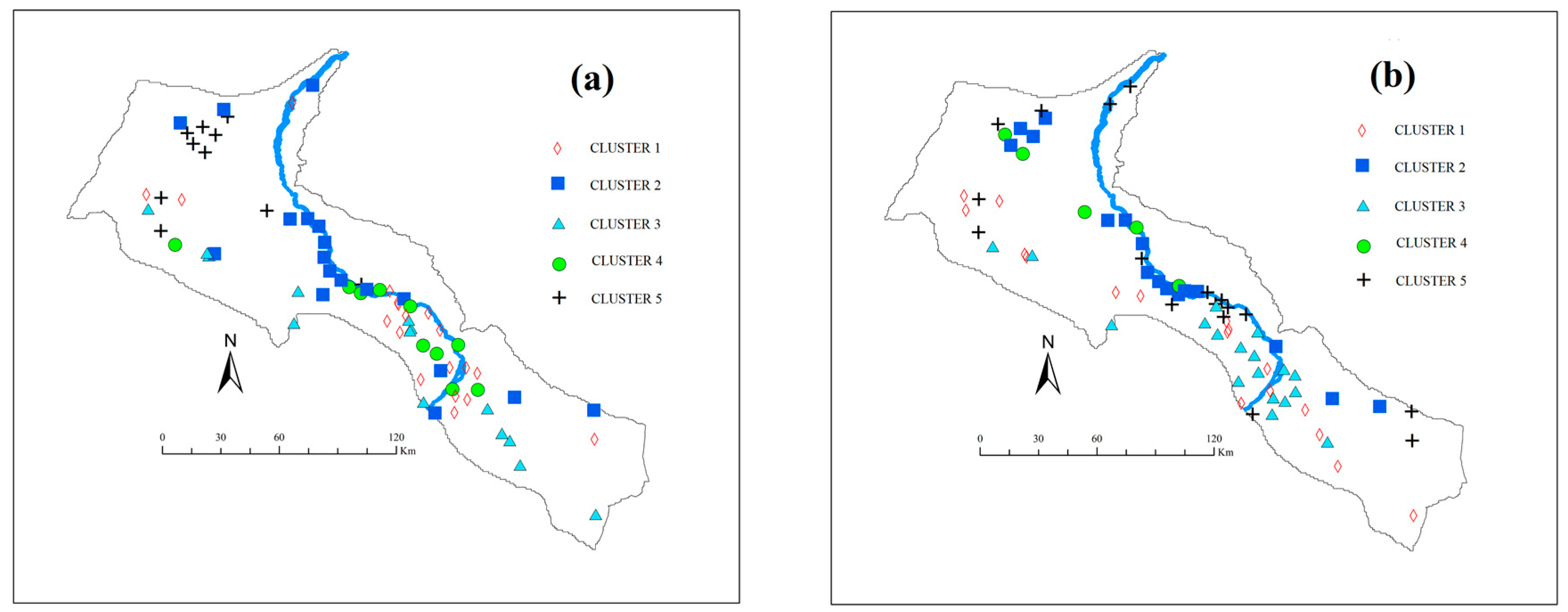
Unfortunately, all heuristic methods have several major weaknesses. First, because “similarity” is defined in heuristic methods in terms of measured distances, such as Euclidean distance [19], observations belonging to similar correlations may be incorrectly grouped if they record long distances. Second, the process of selecting an appropriate clustering method and determining its parameters is usually subjective. There are no quantitative criteria to determine the distance metrics and key clustering parameters, such as the number of clusters and the initial cluster centers. In contrast to heuristic methods, model-based methods do not use distance measures. Instead, these models assume that a given dataset contains several sub-populations that should be modeled separately and that the overall population represents a mixture of these subpopulations [20]. Observations belonging to the same sub-population should enter the same cluster. Each sub-population can be represented by a parametric distribution (e.g., a Gaussian distribution), and the entire dataset can be modeled as a mixture of multiple distributions [21]. Because model-based methods are not restricted to distance measures and adopt a rigorous probability framework [22], they provide more reliable and meaningful clustering results in certain situations. Figure 1 shows such an example. Additionally, model-based methods can use quantitative criteria, such as the Bayesian Information Criterion (BIC), as objective metrics to determine the best models and number of clusters [23,24]. It has been demonstrated in other fields that model-based methods can overcome the limitations of heuristic methods [20]. However, model-based methods have rarely been applied to hydrological studies [14,25].
Selecting an appropriate probability model is essential for model-based clustering. The Gaussian Mixture Model (GMM) has been widely applied to studies involving pattern recognition and machine learning, information processing, data mining, and clustering [26]. This model has two major advantages: first, it can adequately approximate a broad class of distribution functions, and second, the mathematical form of the GMM simplifies the derivation of the subsequent parameter estimation method [27].
However, the GMM has rarely been adopted in model-based clustering to explore hydrochemical groundwater data. To the authors’ best knowledge, [14] represents the first attempt, but this pioneering application left some important issues to be further investigated. In the case study of [14], the groundwater chemistry was dominated by anthropogenic impacts, and only two ions were considered to be attributes in the final model. Therefore, it remains unclear whether GMM clustering can be used to understand more complicated hydrochemical processes (i.e., processes with both natural and anthropogenic impacts). Additionally, the clusters of groundwater samples studied by [14] did not record clear spatial patterns. Therefore, further work is needed to determine whether GMM clustering can produce an integrated understanding of groundwater chemistry at a large scale.
This study used GMM clustering on a hydrochemical dataset of groundwater samples collected from a semi-arid agricultural area in northwestern China. Its main objectives were to (1) investigate whether and how GMM clustering can be effectively used to address hydrochemical datasets in areas where both natural and anthropogenic factors exert significant effects on groundwater chemistry and (2) demonstrate how GMM clustering can produce an integrated understanding of basin-scale hydrochemical processes with a limited number of observations.

2. Study Area

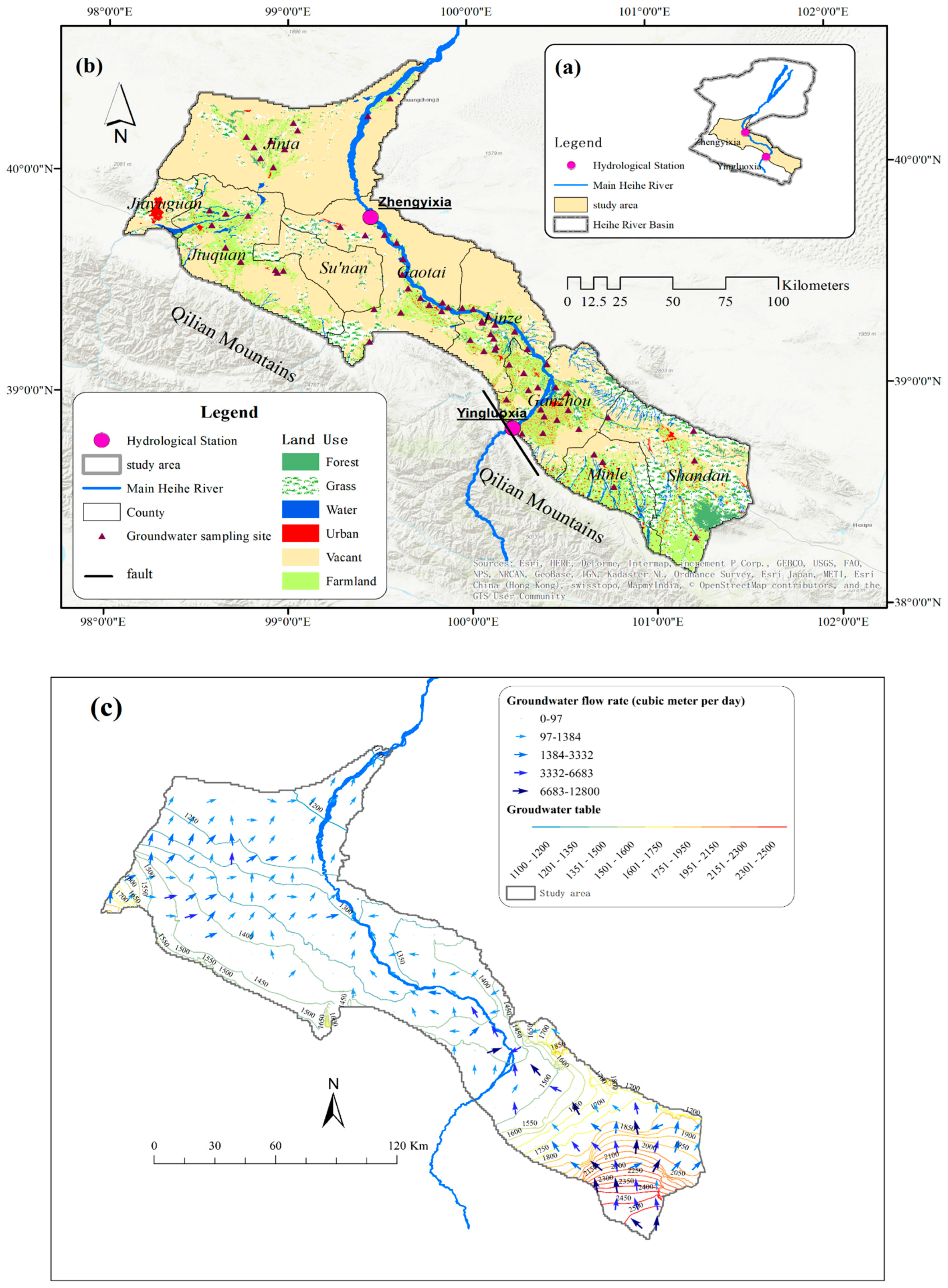
The Heihe River is the second largest inland river in China, with a total length of approximately 900 km. It originates within the Qilian Mountains, flows north and terminates at East Juyan Lake. The entire Heihe River Basin (HRB) (Figure 2a) consists of three distinctive parts: the mountainous upstream area, which is mainly located in Qinghai Province, the semi-arid midstream area with intensive oasis agriculture, which is mainly located in Gansu Province, and the downstream area, which mainly comprises the vast Gobi Desert in Inner Mongolia. On the main river, Yingluoxia and Zhengyixia (Figure 2b) are the separating points of upstream-midstream and midstream-downstream, respectively. With a total area of approximately 130,000 km2, the HRB has an arid continental climate; its annual precipitation ranges from 50 to 300 mm. The Heihe River has more than thirteen tributaries, but some have lost their surface water connections with the main river. The interactions between surface water and groundwater are substantial and complex in the HRB [28]. The HRB has been affected by significant human-nature water conflicts (i.e., midstream vs. downstream, and agriculture vs. ecological services), as discussed in previous studies [28,29,30].
This study focuses on the midstream area of HRB (Figure 2), which is a major part of the Hexi Corridor, a region that was once crossed by the famous ancient “Silk Road”. Its annual precipitation is only 100–150 mm, but it receives a significant amount of surface runoff from the Qilian Mountains, where the annual precipitation exceeds 350 mm [31]. The middle HRB has a long history of irrigated agriculture in its oases. Based on the water resource reports of the local government, farmlands have rapidly expanded over the past several decades, with agriculture now consuming more than 90% of this region’s water supply. Thus, industrial and domestic water uses have very limited impacts on the hydrological and hydrochemical processes in the middle HRB. To secure the environmental flow towards the lower HRB and restore the diminishing terminal lake, the central government enforced a tight restriction on surface water diversion for irrigation in 2000. However, as an immediate response to the flow regulation, groundwater pumping in the middle HRB has increased rapidly since 2000, causing groundwater drawdown and wetlands degradation in some areas.
In the study area, from south to north, the sediments gradually change from coarse-grained gravel to medium and fine-grained sand and then to silt [32,33]. A fault along the foot of the Qilian Mountains largely prevents groundwater from flowing from the mountains into the basin laterally. Thus, streams from the mountain area are the main recharge source for the aquifers. In the south part of Minle County, the aquifer is formed from highly permeable cobble and gravel deposits with a thickness more than 200 m. The depths to the water table range from 50 to 200 m in Ganzhou district and 0.5–5 m in the north part of the floodplain (Linze and Gaotai Counties). Groundwater discharges to river or as springs at the middle part of the study area. In our previous study, we performed integrated surface water-groundwater modeling using GSFLOW [34] to study the complex water cycle of the HRB and its response to human activities [29,31,35]. It has been found that this area has significant surface water-groundwater interaction, and the interaction is complicated by intensive pumping and irrigation [30,31,35]. Figure 2c plots the groundwater table and flow directions based on Tian et al.’s model [28].
The surface water salinity increases from upstream to downstream, and the water type shifted gradually from HCO3, SO42− to Cl, mostly due to water-rock interactions [10,36,37,38], which is typical of arid to semi-arid areas. Nonetheless, little attention has been paid to the groundwater chemistry of this region. Some studies [10,32,33,39] provided basic descriptions of the hydrochemical features of the entire basin, but none have performed in-depth investigations of the agricultural area in the middle HRB. Additionally, the previous studies mostly discussed natural chemical evolution processes while overlooking anthropogenic impacts. How the agricultural activities, such as diversion, pumping, irrigation and fertilization, would impact the groundwater chemistry deserves further investigation.

3. Materials and Methods

3.1. Sample Collection and Treatment

This study focuses on groundwater used for agricultural irrigation. In a field campaign in August 2014, 73 groundwater samples were collected from irrigation wells (see Figure 2b) in Zhangye, Jiuquan and Jinta Counties, which contain the majority of the population and agriculture in the middle HRB. These wells were created for irrigation and mainly draw water from the uppermost aquifer, which can provide sufficient groundwater for irrigation. Most of these irrigation wells pump groundwater from unconfined shallow aquifers (in which the groundwater depth varies from 0.7 to 170 m) that interact with surface water. Therefore, these samples record important information about anthropogenic impacts on the groundwater system. A few irrigation wells in Minle County (Figure 2) draw groundwater at depths of 200–300 m.
At each sampling site, groundwater was pumped out for more than 15 min before any samples were taken to clean the well tube. In the field, HCO3 and CO32 contents were determined using titration; and electrical conductivity, temperature and pH were measured using portable equipment. When collecting samples for laboratory analysis, water was first filtered using a 45-μm cellulose membrane and stored in an acid-cleaned 30-mL high-density polyethylene (HDPE) bottle. Samples were stored in a cooler and then transferred to a refrigerator on the same day. All samples were measured for Na+, Mg2+, Ca2+, K+, Cl, and NO3 in the laboratory. These measurements were conducted at the Geochemistry Laboratory of the Cold and Arid Region Environmental and Engineering Institute, Chinese Academy of Sciences (Lanzhou, Gansu Province, China), following the standard methods developed by the American Public Health Association [40]. Dissolved cations were measured using chromatography (DX-600 of Dionex) by an inductively coupled plasma optical emission spectrometer, and anions were measured using the ICS-2500 chromatograph of Dionex. All analyses followed the same standard methods and were carefully calibrated by an appropriately diluted standard. The accuracy and precision of these measurements were checked by analyses of reference materials. All relative errors are within ±5%.

3.2. GMM Clustering

The GMM considers an entire dataset to be a mixture of K clusters of Gaussian distributions, in which each cluster is associated with a weight ωk. This dataset can be in the form of an observation matrix, X (n × p), where n is the sample size (i.e., the number of observations) and p is the number of attributes. The ith observation is denoted as xi, which represents an independent realization from one of the K clusters. However, it is unknown to which cluster xi belongs [23]. If μk (p × 1) and Dk (p × p) denote the expectation vector and the covariance matrix of the kth cluster (k = 1, 2,…, K), respectively, then we can further define θ k = { μ k , D k } . In this case, all observations are independent identically distributed (IID) vectors, and a mixture probability density function (pdf) (i.e., the probability model), with specific K and p values, can be written as
G ( x ) = k = 1 k ω k g k ( x | μ k , D k )
where gk represents the kth Gaussian distribution and can be further written as [23]:
g k ( x | μ k , D k ) = 1 ( 2 π ) p / 2 | D k | 1 / 2 e x p [ 1 2 ( x μ k ) T D k 1 ( x μ k ) ]
The entire parameter set, Θ = { θ 1 , θ k , ω 1 , ω k } , can be estimated using a maximum likelihood estimation (MLE) approach. We first define a label vector zik. If the ith observation comes from the kth cluster, then zik = 1; otherwise, zik = 0. Because the observations are IID, the likelihood function can be defined as
M a x Θ    L ( Θ , X ) = i = 1 n l n [ k = 1 k z i k ω i k g k ( x i | μ i , D k ) ]
In Equation (3), direct MLE is not feasible because the cluster label zik is unobserved. In such cases, the Expectation-Maximization (EM) algorithm [41] can be applied to obtain the optimal Θ , as introduced in Section 3.4.
After the MLE is completed, the membership probability of each observation belonging to the kth cluster, denoted as mik, can be calculated as [21]:
m i k = ω k g k ( x i | μ i , D k ) t = 1 k ω t g t ( x i | μ i , D t )
It holds that k = 1 k m i k = 1 . The ith observation can then be assigned to the cluster with the highest membership probability. The label zik can then be determined as
z i k = { 1 , m i k =    a r g m a x s { 1 , , k } ( m i s ) 0 , o t h e r w i s e
Additionally, for each observation, the clustering uncertainty can be calculated as [6]:
U C i = 1 M a x k m i k
In order to demonstrate the advantage of GMM clustering, k-means clustering, an approach widely used in various fields including hydrology [18], was also performed and compared with GMM clustering. The technical details of K-means clustering can be found elsewhere [42,43].

3.3. Model Selection

Selecting the appropriate K and p attributes is critical to the performance of the GMM clustering. Once the values of the K and p attributes are determined, the structure of the probability model (i.e., Equation (1)) is fixed, and MLE can be performed to further estimate the parameter set Θ = { θ 1 , θ k , ω 1 , ω k } . In this study, the Bayesian Information Criterion (BIC) was used to determine the K value and p attributes and is formulated as [24]:
BIC = 2 L + λ l n ( n )
where L is the log-likelihood estimated by MLE (Equation (3)), λ is the number of parameters to be estimated, and n is the sample size (n = 73). Each cluster model with p selected attributes and a specific value of K achieves a BIC score; the model with the lowest BIC score can be interpreted as the best model [44].
In the GMM, λ can be calculated as [23]:
λ = K p + p ( p + 1 ) k 2 + K 1
The first item in this equation represents the total number of elements in the K expectation vectors (μk), and the second item represents the total number of covariance coefficients contained in all the Dk’s. Obviously, λ increases rapidly with both K and p, which can lead to an increase of the BIC score, unless there is a significant improvement in L.
As a model-based clustering method, GMM clustering also suffers from the “curse of dimensionality” because it is likely to cause over-parametrization in high-dimensional spaces [23,45]. Data preprocessing for dimension reduction is one solution to overcome this obstacle [46], and a classic technique is principal component analysis (PCA) [47]. In some applications, primal variables are more suitable for clustering than principle components [14]. In this study, to find a suitable set of p attributes for clustering, both the primal concentration variables and their principle components (PCs) were considered candidate attributes. Hydrochemical data often follow non-normal distributions, and therefore appropriate data processing is necessary before any parametric analyses [48]. In this study, PCA was conducted for the standardized logarithms of the concentrations, as is commonly done in hydrochemical studies [16].

3.4. Expectation-Maximization Algorithm

The well-known EM algorithm can solve MLE problems using unobserved variables, and it has previously been applied to GMM clustering [48,49]. In this case, Θ = { θ 1 , θ k , ω 1 , ω k } is the parameter set to be estimated via MLE, where θ k = { μ k , D k } represents the parameters of the kth Gaussian distribution. Referring to Equation (5), zik is an unobserved variable depending on the dataset Xn×p and the parameter set Θ . If t denotes the iteration number and the initial t = 0, then the key steps of the EM algorithm can be summarized as follows.
Step 1: Randomly initialize Θ ^ ( 0 ) = { θ 1 ( 0 ) , θ k ( 0 ) , ω 1 ( 0 ) , ω k ( 0 ) } .
Step 2: (E-step): Based on θ ^ ( t ) , estimate the expectation (denoted as z ^ i k ( t ) ) of zik as
z ^ i k ( t ) = E [ z i k | Θ ^ ( t ) , x ] = P r o b ( z i k | Θ ^ ( t ) , x ) = ω ^ k ( t ) g ( x i | θ ^ k ( t ) ) j = 1 k ω ^ j ( t ) g ( x i | θ ^ j ( t ) )
Step 3: (M-step): Update the parameter set as follows.
ω ^ k ( t + 1 ) = i = 1 n z ^ i k ( t ) n
μ ^ k ( t + 1 ) = i = 1 n z ^ i k ( t ) x i i = 1 n z ^ i k ( t )
D ^ k ( t + 1 ) = i = 1 n z ^ i k ( t ) ( x i μ ^ k ( t + 1 ) ) ( x i μ ^ k ( t + 1 ) ) T i = 1 n z ^ i k ( t )
Step 4: Calculate the likelihood L using Equation (3). Set t = t + 1, and repeat Step 2 and Step 3 until the convergence condition is satisfied. A general convergence requirement is to reach | L ( t + 1 ) L ( t ) | < ε . ε is a threshold that was set to 0.01 in our study.
More details of the EM algorithm can be found elsewhere [41,49]. This algorithm is sensitive to the initial parameter values (i.e., Θ ^ ( 0 ) ) and usually requires a large number of initial points to achieve adequate MLE results. In this study, for each candidate GMM, the EM calculation was repeated 10,000 times with randomly generated initial points. The estimated Θ value yielding the lowest BIC score was then considered the optimal parameter value for the model.
All the above analyses were conducted using MATLAB. The MATLAB code of GMM-EM is provided by https://github.com/HammerZhang/GMM. The kmeans function in MATLAB was used to perform k-means clustering.

4. Results and Discussion

4.1. Descriptive Statistics

For our samples, the concentration of total dissolved solids (TDS) ranges from 307.6 to 4164.6 mg/L, with an average value of 1245.6 mg/L. According to [50], 15 samples can be categorized as non-saline drinking and irrigation water (TDS ≤ 500 mg/L), 40 samples as slightly saline irrigation water (500 mg/L < TDS ≤ 1500 mg/L), and 18 samples as moderately saline, primary drainage water (1500 mg/L < TDS ≤ 7000 mg/L). The concentrations of TDS and individual ions were first log-transformed, and then standardized to have zero mean and unit variance. Kolmogorov–Smirnov tests performed with MATLAB validated that the transformed concentration data follow a standard normal distribution. For Na+, K+, Mg2+, Ca2+, Cl, SO42−, NO3 and HCO3, the p-values of Kolmogorov–Smirnov test are 0.0994, 0.433, 0.501, 0.581, 0.054, 0.399, 0.068 and 0.223, respectively. Thus, the hypothesis that the transformed concentrations follow a standard normal distribution cannot be denied at the confidence level of α = 0.95, and parametric statistics are applicable to the transformed data.
Table 1 presents the Pearson correlation coefficient matrix of the log-transformed concentrations. NO3 does not show any significant correlation with other variables, with all p-values higher than 0.05. All other pairs record significant correlations, with p-values less than 0.01. In particular, the pairs of Na+-Cl, Mg2+-Ca2+, Na2+-SO42−, Cl2+-SO42− and Mg2+-SO42− have correlation coefficients greater than 0.85. In fact, we also calculated Spearman’s rank correlation coefficients [51,52]. The nonparametric results are very similar to the parametric ones, except that weak correlation between NO3 and several cations is identified.
In a typical arid and semi-arid river basin, most ions would have a tendency to increase from upstream to downstream because of the rock weathering and lixiviation processes. Our data also reflect this tendency. The correlation between TDS and the ions are all positive, and the correlation coefficients are very high, mostly above 0.8, except those for K+, NO3 and HCO3. K+ has similar properties as Na+, but its abundance in natural waters is much lower [52], and it is intensively absorbed by plants [53]. NO3 in groundwater is not significantly influenced by rock-water interactions. Instead, it reflects the influences of anthropogenic activities, such as fertilization in irrigated farmlands, where excessive nitrate may leach into groundwater [14,54]. Among the 73 samples, 8 samples have NO3 concentrations greater than 44.3 mg/L, which exceed the drinking water standards defined by the WHO. For HCO3, the dominating impact of rock-water interactions may be reduced by the infiltration, which can transport surface water with relatively abundant dissolved CO2 (generated by plant respiration and organic matter decay) to the groundwater [55]. As these results indicate, the hydrochemical features of the groundwater are likely influenced by many processes, including rock weathering and lixiviation processes, fertilization, plant uptake, and surface water-groundwater interactions.

4.2. PCA Results

As Table 2 shows, the top four PCs individually explain 61.5%, 14.4%, 11.5% and 7.5% of the total variance and collectively explain 94.8% of the variance. Thus, PCA has successfully reduced the data dimension from 8 to 4. As shown by Table 2, PC1 has high positive loadings in Na+, K+, Mg2+, Ca2+, Cl and SO42− but very low loadings in HCO3 and NO3. Additionally, PC1 has a strong linear relationship with TDS (R2 = 0.956). Therefore, PC1 is likely an indicator of salinity and can be used to represent rock-groundwater interactions. PC2 has very high positive loadings in NO3 and HCO3 and negative loadings in SO42−, Na+ and Cl. As previously mentioned, NO3 and HCO3 in groundwater reflect the influence of surface water. In addition, previous studies [56] have found that the SO42− and Cl contents in surface water were significantly lower than those in the nearby groundwater. Thus, PC2 can indicate the influence of surface water and represent the surface water and groundwater interaction. PC3 features a high positive loading in HCO3 and a high negative loading in NO3. It may thus reflect the relative importance of natural and anthropogenic impacts on groundwater chemistry. In an agricultural area such as the middle HRB, fertilization can contribute a significant amount of NO3 to shallow groundwater through surface water infiltration and groundwater recharge [14]. Therefore, a high PC3 score indicates that the groundwater has not been significantly impacted by fertilization. PC4 has a high positive loading in Na+ and high negative loadings in other three cations: Ca2+, K+ and Mg2+. Therefore, it may represent the cation exchange process of clay particles, which is common in arid and semi-arid environments [53,54,57].

4.3. Clustering Results

Candidate models with different K values and attribute sets were examined, and Table 3 shows the likelihood and BIC values associated with the twelve models. Models 1 to 9 record different combinations of K values and PCs, and Models 10 and 11 consider Cl, NO3 and HCO3 as its three attributes. These three ions are selected because their correlations are relatively weak (Table 1) and may represent distinctive aspects of hydrochemical processes. Model 12 considers all ions except SO42− and Na+ and the pH as its attributes. SO42− is excluded because its concentration is linearly related to those of Cl, Na+ and Mg2+ (Table 1). Similarly, Na+ concentration is linearly related to that of Cl. Among all of the candidate models, Model 7 has the lowest BIC value (195.00) and is therefore considered to be the best model. In this model, PC1, PC2 and PC3 form the best set of attributes, and the appropriate number of cluster is 6. It is clear that the PCA effectively reduces the data dimensions from eight to three and significantly improves the overall clustering performance. These three PCs can explain over 90% of the total variance. In [14], the first four PCs explained no more than 80% of the total variance, which may be why primal variables outperformed PCs. In addition, the result of Model 12 proves the necessity of dimension reduction before clustering.
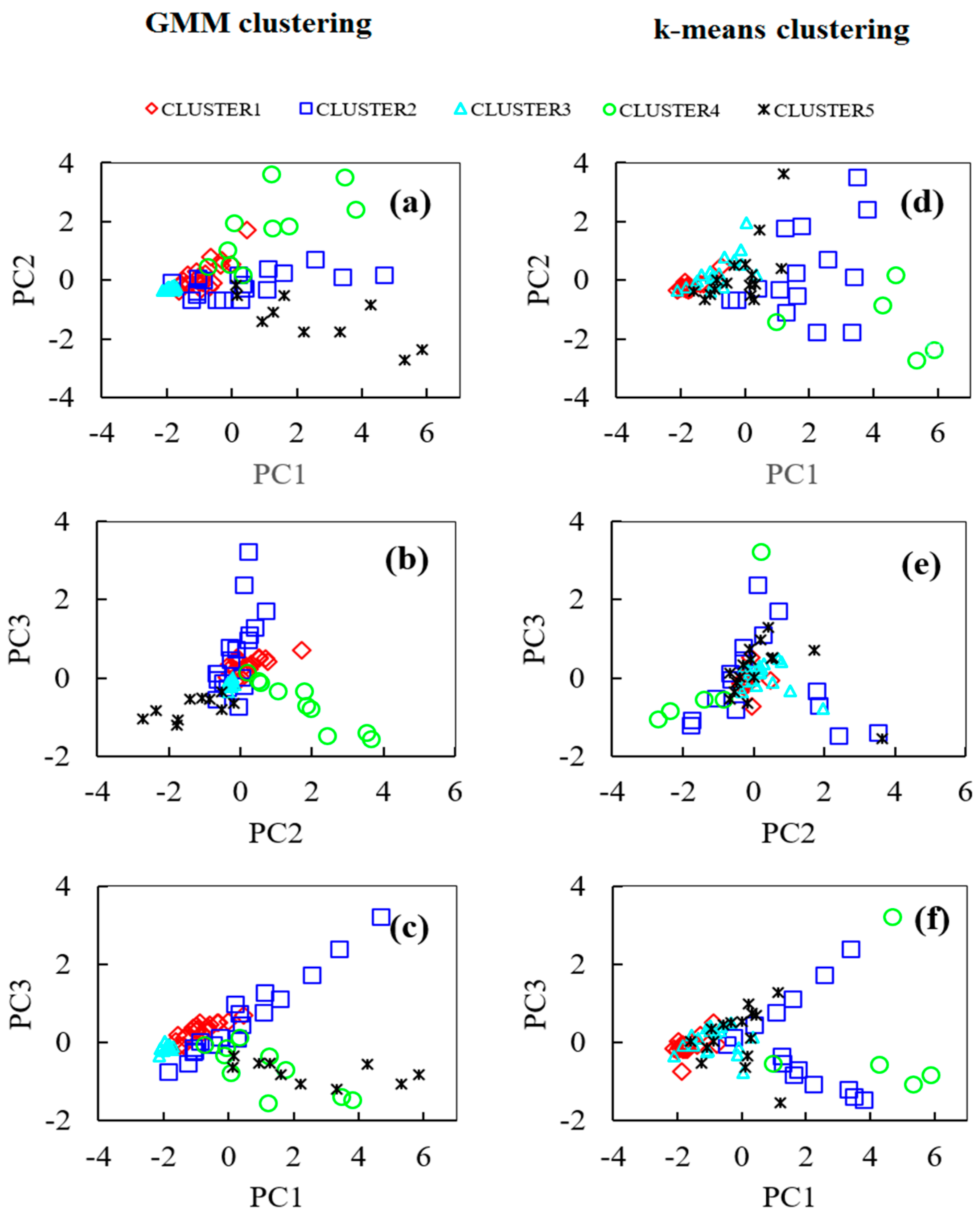
Figure 3a–c illustrate the PC scores of the first five clusters based on Model 7 of GMM clustering. Compared to Model 6 which identifies fiver clusters, Model 7 separates two samples from the second cluster to form the sixth cluster, leading to a lower (i.e., better) BIC. All the first five clusters show significant correlations between the PC scores. With only two samples, the sixth cluster demonstrates no pattern, and is therefore excluded from our discussion and not presented in Figure 3. For comparison, the results of k-means clustering are presented in Figure 3d–f. This classic approach is based on distance, usually Euclidean distance, and requires the number of clusters be pre-defined. Interestingly, when we set the number of clusters to six, the same two points forms a separate cluster. Thus, Figure 3d–f also plot five clusters. It is evident that the clusters based on k-means clustering show no clear patterns in the PC spaces. Thus, the comparison in Figure 3 clearly reflects the advantage of GMM clustering in pattern recognition (refer to Figure 1). This advantage would enable a sophisticated interpretation of the hydrochemical processes.
As was discussed before, PC1, PC2 and PC3 indicate salinity (positive relationship), the influence of surface water (positive relationship) and the impact of fertilization (negative relationship), respectively. In the PC1-PC2 space (Figure 3a), a positive (negative) relationship between PC1 and PC2 may indicate that surface water recharge enhances (reduces) groundwater salinity. In the PC2-PC3 space (Figure 3b), a negative relationship between PC2 and PC3 may suggest that groundwater is receiving fertilization-impacted surface water, which is only evidence for CLUSTER 4. In the PC1-PC3 space (Figure 3c), a negative relationship between PC1 and PC3 (most evident in CLUSTER 4) may indicate that fertilization enhances groundwater salinity. In contrast, the positive relationship between PC1 and PC3 (most evident in CLUSTER 2) probably reflects a common situation in arid areas that high salinity of irrigation water can limit agricultural development [58,59]. According to our field investigation and existing studies [60], the agricultural productivity of the farmlands along the river within Gaotai County, where the samples in CLUSTER 2 are located, is indeed influenced by salinity.
Table 4 summarizes the main features of the five clusters demonstrated in Figure 3a–c. The groundwater in CLUSTER 1 has a moderate level of salinity (indicated by PC1), which can be enhanced by surface water recharge (indicated by PC2 and the PC1-PC2 relationship). Although salinity is influenced by fertilization (indicated by PC3), its effect is not through the recharge from surface water (indicated by PC2-PC3 relationship) but is probably through lateral groundwater flow. In CLUSTER 1, groundwater salinity may limit agricultural development (as indicated by the PC1-PC3 relationship). Compared to CLUSTER 1, CLUSTER 2 has a much wider range in salinity (as indicated by PC1), but the variation in salinity is not due to the recharge (indicated by PC1-PC2 relationship). The impact of fertilization is weaker in CLUSTER 2 than it is in CLUSTER 1 (as indicated by PC3). CLUSTER 3 has the lowest salinity (as indicated by PC1). Although surface water does influence groundwater chemistry (as indicated by PC2), it does not significantly change groundwater salinity (as indicated by the PC1-PC2 relationship). There is also no evident connection between groundwater quality and agricultural development in this case (as indicated by the PC1-PC3 relationship). As in CLUSTER 1, although the salinity in CLUSTER 3 is influenced by fertilization (as indicated by PC3), this effect is likely due to horizontal groundwater flow instead of surface water recharge. For CLUSTER 4, a distinctive characteristic is the fertilization-impact recharge (as indicated by PC3), which enhances groundwater salinity (as indicated by PC1 and the PC1-PC2 relationship) and degrades the quality of the groundwater (as indicated by the PC1-PC3 relationship). CLUSTER 5 has the highest salinity level of all five clusters (as indicated by PC1), which can be reduced by recharge (as indicated by the PC1-PC2 relationship), probably because the recharge water has a much lower salinity than the groundwater. The chemistry of the groundwater is also influenced by fertilization (as indicated by PC3), which has a (indicated by PC2 and PC2-PC3 relationship) but instead from horizontal groundwater flow degrading effect (as indicated by the PC1-PC3 relationship). However, this influence may be not from recharge that brings nitrogen from further upstream in the groundwater flow field.
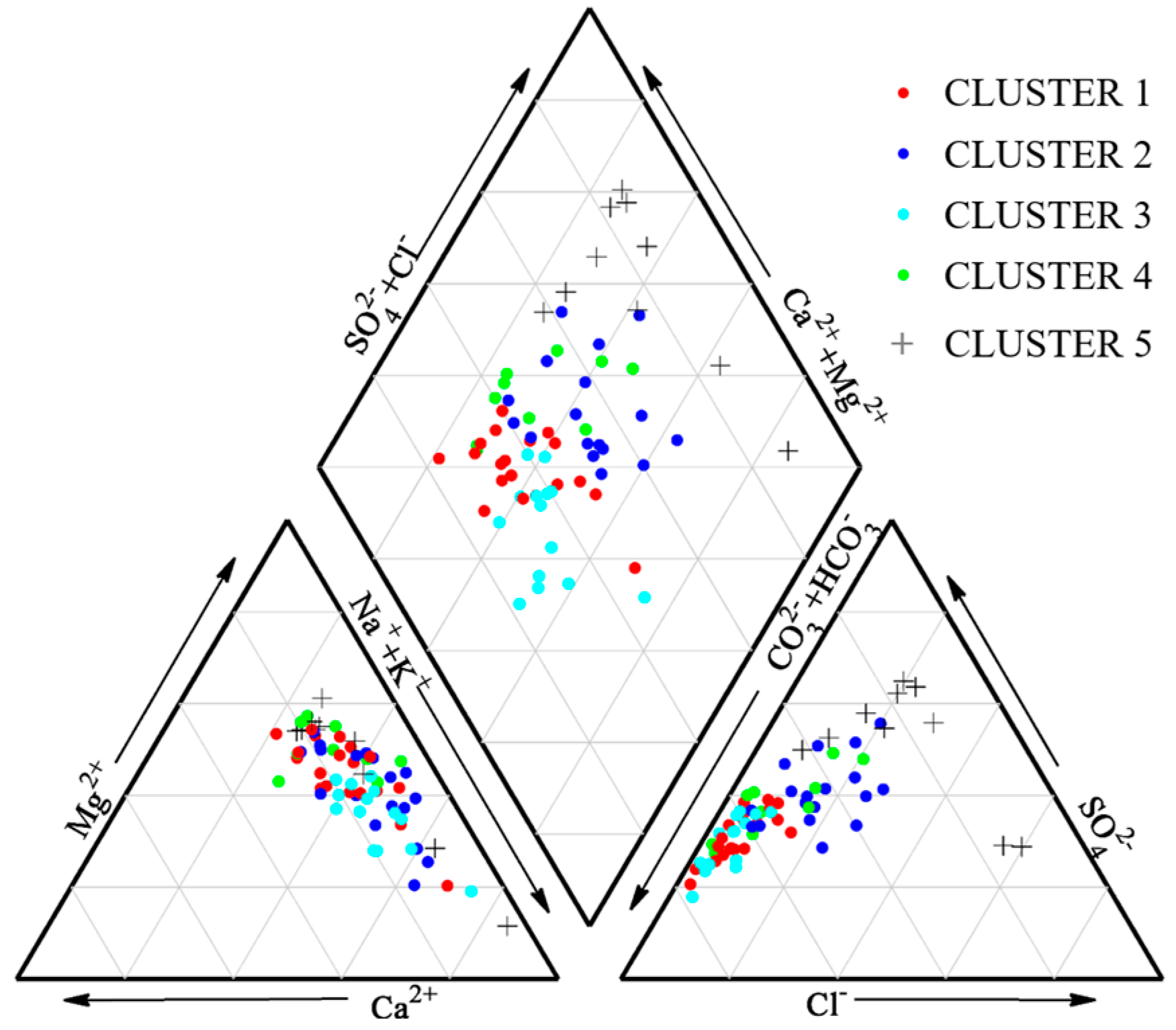
A Piper diagram was also created for all groundwater samples (Figure 4). The fact that the five clusters are much better separated in the anion space implies that anions, rather than cations, determine the spatial variation of groundwater chemistry in this area. Both CLUSTER 3 and CLUSTER 1 have low salinities and relatively high HCO3 contents. In contrast, CLUSTER 5 has very high salinity dominated by SO42− and Cl. CLUSTER 2 and CLUSTER 4 are between the extremes and are not well partitioned in the anion space because NO3 was not included in the Piper diagram. The transition of CLUSTER 3 → CLUSTER 1 → CLUSTER 2 → CLUSTER 5 reflects a common natural salinization process that occurs from upstream to downstream in semi-arid basins [33,39], whereas CLUSTER 4 mainly reflects the impact of agriculture.
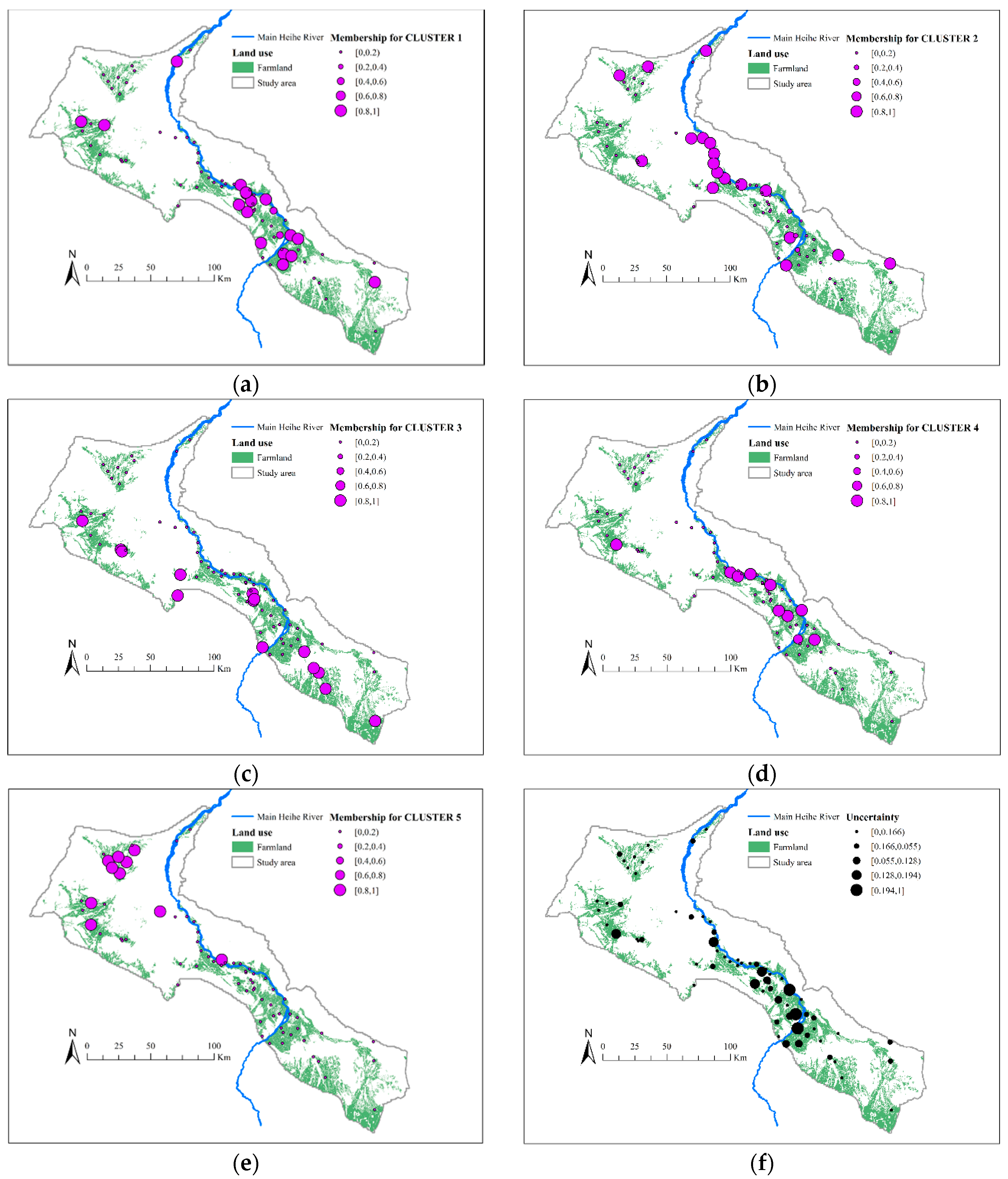
Figure 5 illustrates the spatial and probabilistic details of the clustering results. In Figure 5a–e, the size of each circle indicates the probability that a sample belongs to a given cluster, whereas in Figure 5f, the size of the circle indicates its clustering uncertainty (Equation (6)). Figure 6 illustrates the regional groundwater flow field simulated by an integrated surface water-groundwater model [35]. According to Figure 5, the five clusters have different high-probability locations (HPLs). The HPLs of CLUSTER 1 (Figure 5a) and CLUSTER 4 (Figure 5d) are mixed in Ganzhou District and Linze County, which have intensive agriculture (refer to Figure 2). However, the hydrochemical processes differ significantly between the clusters (see Table 4), as discussed above. The HPLs of CLUSTER 2 (Figure 5b) are mainly located in Gaotai County (Figure 2), which is downstream of the HPLs of CLUSTER 1 and CLUSTER 4, in which farmlands are confined to a narrow strip along the river. The HPLs of CLUSTER 3 (Figure 5c) are distributed in the areas upstream of the regional groundwater flow field (Figure 7). The HPLs of CLUSTER 5 (Figure 5e) are mainly located in Jinta Basin, which is in the most downstream part of the groundwater flow field (Figure 7). These spatial patterns reinforce our previous argument that the transition of CLUSTER 3 → CLUSTER 1 → CLUSTER 2 → CLUSTER 5 reflects the common natural salinization process of groundwater moving from upstream to downstream in semi-arid basins, whereas the data of CLUSTER 4 mainly reflect the impact of agriculture.

4.4. Regionalization of Groundwater Chemistry

Clustering has been widely applied in regionalization studies [6,9,61]. Conversely, reasonable regionalization results can also validate the clustering results [25]. Figure 6 demonstrates that, in this study, GMM clustering has resulted in a much more interpretable spatial pattern than k-means clustering. For example, in Figure 6a, the samples in CLUSTER 4 are concentrated in the productive farmlands, and the samples in CLUSTER 5 are mainly located in the Jinta and Jiuquan Basins. In contrast, based on k-means clustering (Figure 6b), all the five clusters have scattered samples.
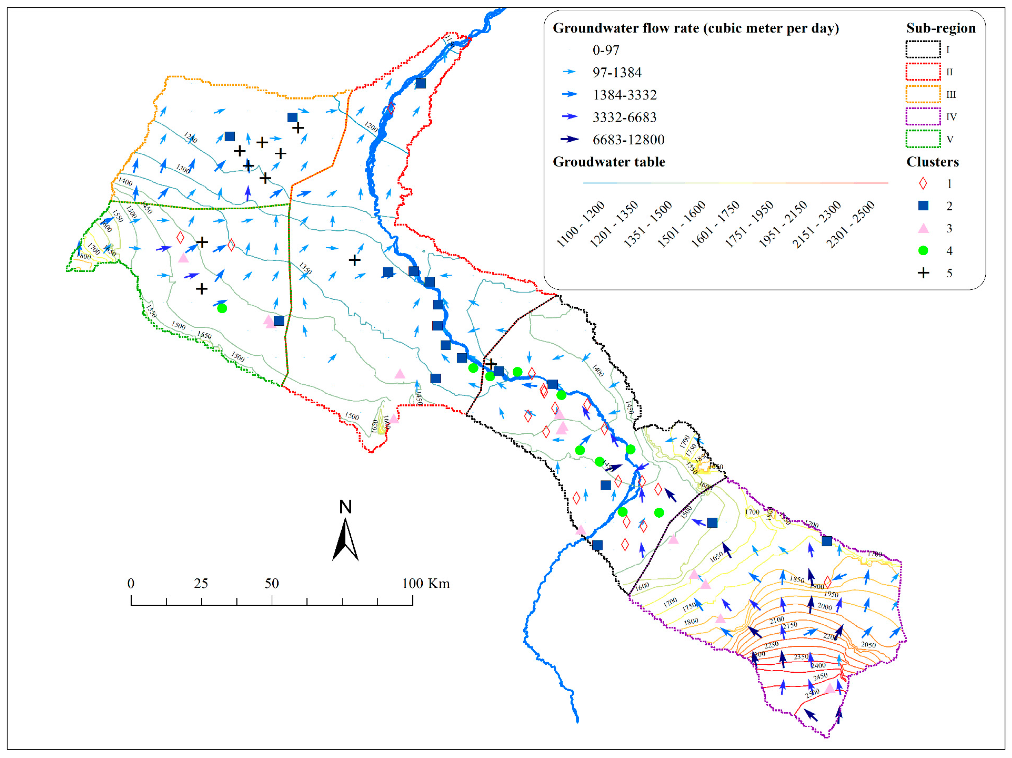
Five sub-regions were further identified, as illustrated in Figure 7. In Sub-region I, CLUSTER 1 and CLUSTER 4 are the major groundwater types. Within these areas, the clustering uncertainty is relatively high (Figure 5f), which implies that this sub-region features a series of highly complicated hydrochemical processes. Sub-region I has very productive farmlands with intensive fertilization, and the surface water-groundwater exchanges in this sub-region are strong in both directions and have been significantly influenced by human activities such as diversion, pumping and irrigation [35]. Additionally, both the surface and subsurface water-rock interactions in Sub-region I are active [10,32,33]. Sub-region II is downstream of Sub-region I. The dominance of CLUSTER 2 in this sub-region (Figure 7) implies that the mixing of surface water and groundwater does not significantly affect groundwater salinity in this area. In fact, the strong water-rock interaction in this area causes salinity to gradually increase from upstream to downstream [56]. In contrast to Sub-region I, this sub-region features a relatively small area of farmland, which is mainly distributed in a narrow strip along the river (Figure 5b); therefore, the anthropogenic effect is not significant.
Sub-region III is mainly located in the Jinta Basin, and is dominated by CLUSTER 2 to CLUSTER 5, the two downstream groundwater types. Both clusters are not significantly impacted by surface water, as is indicated by Table 4, which is consistent with the fact that this sub-region has low precipitation, high evapotranspiration, and a relatively weak hydraulic connection with the main Heihe River (Figure 7). Sub-region IV represents the upstream part of the groundwater flow field, where groundwater salinity is low. The groundwater depth in this region is very deep (200–300 m); therefore, agricultural activities can only weakly influence the groundwater quality. Sub-region V occupies the northwest region of the study area, and mainly includes Jiuquan Basin. It has a mixture of five clusters and is a relatively isolated area with a weak hydraulic connection with the main Heihe River.
Figure 7 shows that GMM clustering produces satisfactory regionalization results, which in turn validate the clustering analysis. Although many regionalization methods, such as the approaches based on the Tyson triangle and Kriging interpolation, rely on the geographical locations of observations, the GMM clustering approach requires no location information. Clearly, GMM clustering can effectively identify connections between observations based on underlying physical processes, rather than geographical distance. Compared to the work [14], the clusters of samples in our study are more spatially assembled, which helps develop an integrated understanding of the regional hydrochemical processes.

4.5. Impact of Regional Water Cycle

To further validate these clustering results, the Spearman’s rank correlation [51] is examined between the membership probabilities calculated by Equation (4) and a series of key hydrological variables representing climatic, topographical and agricultural factors. Here, we further define m k = [ m 1 k , m 2 k , m n k ] T as the membership vector of the kth cluster. Hydrological variables have either been observed (e.g., rainfall, surface water diversion for irrigation) or modeled (e.g., evapotranspiration and infiltration rates) by [35]. This statistical analysis considers the annual average values (from 2000 to 2012) of these variables within the 9-km2 domain in which each sampling site lies (i.e., a 3 × 3 modeling grid with the site in the central square). The rationale behind considering temporally averaged values is that groundwater chemistry undergoes change relatively slowly and thus largely reflects the long-term impacts of hydrological processes [61]. The rationale to perform spatial averaging is that groundwater chemistry may reflect not only the hydrological processes at a specific site but also those in adjacent areas.
Table 5 presents the calculated correlation coefficients of this analysis. These results are consistent with previously discussed findings. First, precipitation is positively correlated with m1, m3 and m4 but has no significant correlation with m2 and m5. Given that Table 4 shows, CLUSTERs 1, 3 and 4 have a common feature that the influence of surface water is at least at a medium level, this correlation with precipitation likely reflects the influence of surface water on groundwater chemistry. Second, in addition to recording a positive correlation with precipitation, m3 demonstrates a negative correlation with potential ET and irrigation and a positive correlation with groundwater depth. As discussed previously, CLUSTER 3 is generally distributed within the upstream area of the groundwater flow field, where elevation and groundwater depth are relatively high and temperature is relatively low. This explains the positive correlation with groundwater depth and the negative correlation with potential ET. Additionally, CLUSTER 3 mainly reflects the upstream stage of the common natural salinization process in semi-arid basins and has little agricultural impact (Table 4), which explains the observed negative correlation with irrigation. Third, in addition to the observed positive correlation with precipitation, m4 positively correlates with infiltration, which is consistent with the finding that CLUSTER 4 is characterized by fertilization-impact recharge (Table 4). Fourth, m5 records a positive correlation with the two ET variables and a negative correlation with unsaturated zone (UZ) recharge. In the HPLs of CLUSTER 5, where the climate is dry and hot, the ET process draws water from the shallow aquifer and soil; the downward percolation of water is limited, which leads to increasing concentrations of chemicals in groundwater. Finally, m2 shows no significant correlation with any of the selected variables, which is consistent with the results in Table 4 and reflects the transitional role of CLUSTER 2 in the natural salinization process of groundwater moving from upstream to downstream in semi-arid basins.
It is evident that by introducing independent hydrological data, the correlation analysis further validated the clustering results. An important implication of this conclusion is that with the GMM clustering analysis conducted in this study, a single sampling campaign can provide ample information about the hydrochemical processes of groundwater.

5. Conclusions

This study applies GMM clustering to a hydrochemical dataset of groundwater collected in the middle Heihe River Basin (HRB) in northwestern China. To validate these clustering results, a regionalization of groundwater chemistry was attempted, and independent hydrological data were introduced to perform correlation analyses. The GMM clustering results and the regionalization results based on this clustering provide ample information about the hydrochemical processes in the study area. The main findings include the following. First, in the middle HRB, groundwater chemistry demonstrates a typical natural salinization process moving from upstream to downstream, in which this natural process is further complicated by anthropogenic factors. Second, regional hydrological processes, especially surface water-groundwater interactions, can exert a profound and spatially varied impact on groundwater chemistry. Third, the interaction between human activity (which, in this study area, is mainly defined as agricultural development) and groundwater quality is complicated. In some farmlands, groundwater quality may be significantly degraded by agricultural development, whereas in others, groundwater quality may constrain this agricultural development.
Overall, this study demonstrates that the GMM can be effectively used in clustering to address hydrochemical groundwater datasets. Additionally, GMM clustering can provide insights into hydrochemical processes, even with a limited number of observations (e.g., the data collected in a single sampling campaign, as in this study). In many remote inland areas, it is technically and financially difficult to implement long-term high-frequency groundwater monitoring, and even a single sampling campaign can be very costly. Therefore, using the clustering approach developed in this study is a cost-effective way to investigate the groundwater chemistry in such areas. Future studies may address the following important issues: (1) dealing with multiple periods of data in the GMM clustering; (2) fusing hydrochemical and hydrological data in the GMM clustering; and (3) automating the selection of the optimal model.

Acknowledgments

This work was funded by the National Natural Science Foundation of China (No. 41622111; No. 91647201; No. 41501024), and Shenzhen Science and Technology Innovation Commission (No. JCYJ20160530190411804). Additional support was provided by the Southern University of Science and Technology (No. G01296001). The data used in this study, if not collected by the authors or acknowledged in the text, were provided by the Heihe Program Data Management Center (http://www.heihedata.org).

Author Contributions

Yi Zheng, Xin Wu, and Yong Tian designed the study; Bin Wu and Sai Wang led the field work; and Juan Zhang led the laboratory work. All the authors contributed significantly to the sample collection during the field work. Xin Wu and Yi Zheng analyzed the data and wrote the paper.

Conflicts of Interest

The authors declare no conflict of interest.

References

  1. Cloutier, V.; Lefebvre, R.; Therrien, R.; Savard, M.M. Multivariate statistical analysis of geochemical data as indicative of the hydrogeochemical evolution of groundwater in a sedimentary rock aquifer system. J. Hydrol. 2008, 353, 294–313. [Google Scholar] [CrossRef]
  2. Hussein, M. Hydrochemical evaluation of groundwater in the Blue Nile basin, eastern Sudan, using conventional and multivariate techniques. Hydrogeol. J. 2003, 12, 144–158. [Google Scholar] [CrossRef]
  3. Suk, H.; Lee, K.-K. Characterization of a ground water hydrochemical system through multivariate analysis: Clustering into ground water zones. Ground Water 1999, 37, 358–366. [Google Scholar] [CrossRef]
  4. Lee, J.Y.; Cheon, J.Y.; Lee, K.K.; Lee, S.Y.; Lee, M.H. Statistical evaluation of geochemical parameter distribution in a ground water system contaminated with petroleum hydrocarbons. J. Environ. Qual. 2001, 30, 1548–1563. [Google Scholar] [CrossRef] [PubMed]
  5. Güler, C.; Thyne, G.D.; McCray, J.E.; Turner, A.K. Evaluation of graphical and multivariate statistical methods for classification of water chemistry data. Hydrogeol. J. 2002, 10, 455–474. [Google Scholar] [CrossRef]
  6. Cowpertwait, P.S.P. A regionalization method based on a cluster probability model. Water Resour. Res. 2011, 47, W11525. [Google Scholar] [CrossRef]
  7. Yoo, J.; Kwon, H.-H.; Kim, T.-W.; Ahn, J.-H. Drought frequency analysis using cluster analysis and bivariate probability distribution. J. Hydrol. 2012, 420, 102–111. [Google Scholar] [CrossRef]
  8. Mather, A.L.; Johnson, R.L. Event-based prediction of stream turbidity using a combined cluster analysis and classification tree approach. J. Hydrol. 2015, 530, 751–761. [Google Scholar] [CrossRef]
  9. Rao, A.R.; Srinivas, V.V. Regionalization of watersheds by fuzzy cluster analysis. J. Hydrol. 2006, 318, 57–79. [Google Scholar] [CrossRef]
  10. Zhu, G.; Su, Y.; Huang, C.; Qi., F.; Liu, Z. Hydrogeochemical processes in the groundwater environment of Heihe River Basin, Northwest China. Environ. Earth Sci. 2010, 60, 139–153. [Google Scholar]
  11. Kumar, M.; Ramanathan, A.; Keshari, A.K. Understanding the extent of interactions between groundwater and surface water through major ion chemistry and multivariate statistical techniques. Hydrol. Process. 2009, 23, 297–310. [Google Scholar] [CrossRef]
  12. Alvarez, M.D.P.; Carol, E.; Dapena, C. The role of evapotranspiration in the groundwater hydrochemistry of an arid coastal wetland (Peninsula Valdes, Argentina). Sci. Total Environ. 2015, 506, 299–307. [Google Scholar] [CrossRef] [PubMed]
  13. Kim, Y.; Lee, K.-S.; Koh, D.-C.; Lee, D.-H.; Lee, S.-G.; Park, W.-B.; Koh, G.-W.; Woo, N.-C. Hydrogeochemical and isotopic evidence of groundwater salinization in a coastal aquifer: A case study in Jeju Volcanic Island, Korea. J. Hydrol. 2003, 270, 282–294. [Google Scholar] [CrossRef]
  14. Kim, K.-H.; Yun, S.-T.; Park, S.-S.; Joo, Y.; Kim, T.-S. Model-based clustering of hydrochemical data to demarcate natural versus human impacts on bedrock groundwater quality in rural areas, South Korea. J. Hydrol. 2014, 519, 626–636. [Google Scholar] [CrossRef]
  15. Güler, C.; Kurt, M.A.; Alpaslan, M.; Akbulut, C. Assessment of the impact of anthropogenic activities on the groundwater hydrology and chemistry in tarsus coastal plain (Mersin, Turkey) using fuzzy clustering, multivariate statistics and GIS techniques. J. Hydrol. 2012, 414, 435–451. [Google Scholar] [CrossRef]
  16. Güler, C.; Thyne, G.D. Delineation of hydrochemical facies distribution in a regional groundwater system by means of fuzzy c-means clustering. Water Resour. Res. 2004, 40, W12503. [Google Scholar] [CrossRef]
  17. Yidana, S.M.; Banoeng-Yakubo, B.; Akabzaa, T.; Asiedu, D. Characterization of the groundwater flow regime and hydrochemistry of groundwater from the buem formation, Eastern Ghana. Hydrol. Process. 2011, 25, 2288–2301. [Google Scholar] [CrossRef]
  18. Ay, M.; Kisi, O. Modelling of chemical oxygen demand by using ANNS, ANFIS and k-means clustering techniques. J. Hydrol. 2014, 511, 279–289. [Google Scholar] [CrossRef]
  19. Ward, J.H. Hierarchical grouping to optimize an objective function. J. Am. Stat. Assoc. 1963, 58, 236. [Google Scholar] [CrossRef]
  20. Fraley, C.; Raftery, A.E. Model-based clustering, discriminant analysis, and density estimation. J. Am. Stat. Assoc. 2002, 97, 611–631. [Google Scholar] [CrossRef]
  21. Maugis, C.; Celeux, G.; Martin-Magniette, M.-L. Variable selection for clustering with Gaussian mixture models. Biometrics 2009, 65, 701–709. [Google Scholar] [CrossRef] [PubMed]
  22. Bouveyron, C.; Brunet-Saumard, C. Model-based clustering of high-dimensional data: A review. Comput. Stat. Data Anal. 2014, 71, 52–78. [Google Scholar] [CrossRef] [Green Version]
  23. Biernacki, C.; Govaert, G. Choosing models in model-based clustering and discriminant analysis. J. Stat. Comput. Simul. 1999, 64, 49–71. [Google Scholar] [CrossRef]
  24. Fraley, C. How many clusters? Which clustering method? Answers via model-based cluster analysis. Comput. J. 1998, 41, 578–588. [Google Scholar] [CrossRef]
  25. Templ, M.; Filzmoser, P.; Reimann, C. Cluster analysis applied to regional geochemical data: Problems and possibilities. Appl. Geochem. 2008, 23, 2198–2213. [Google Scholar] [CrossRef]
  26. Law, M.H.C.; Figueiredo, M.A.T.; Jain, A.K. Simultaneous feature selection and clustering using mixture models. IEEE Trans. Pattern Anal. Mach. Intell. 2004, 26, 1154–1166. [Google Scholar] [CrossRef] [PubMed]
  27. He, J. Mixture model based multivariate statistical analysis of multiply censored environmental data. Adv. Water Resour. 2013, 59, 15–24. [Google Scholar] [CrossRef]
  28. Tian, Y.; Zheng, Y.; Zheng, C.; Xiao, H.; Fan, W.; Zou, S.; Wu, B.; Yao, Y.; Zhang, A.; Liu, J. Exploring scale-dependent ecohydrological responses in a large endorheic river basin through integrated surface water-groundwater modeling. Water Resour. Res. 2015, 51, 4065–4085. [Google Scholar] [CrossRef]
  29. Wu, B.; Zheng, Y.; Wu, X.; Tian, Y.; Han, F.; Liu, J.; Zheng, C. Optimizing water resources management in large river basins with integrated surface water-groundwater modeling: A surrogate-based approach. Water Resour. Res. 2015, 51, 2153–2173. [Google Scholar] [CrossRef]
  30. Wu, X.; Zheng, Y.; Wu, B.; Tian, Y.; Han, F.; Zheng, C. Optimizing conjunctive use of surface water and groundwater for irrigation to address human-nature water conflicts: A surrogate modeling approach. Agric. Water Manag. 2016, 163, 380–392. [Google Scholar] [CrossRef]
  31. Wu, B.; Zheng, Y.; Tian, Y.; Wu, X.; Yao, Y.; Han, F.; Liu, J.; Zheng, C. Systematic assessment of the uncertainty in integrated surface water-groundwater modeling based on the probabilistic collocation method. Water Resour. Res. 2014, 50, 5848–5865. [Google Scholar] [CrossRef]
  32. Chang, J.A.; Wang, G.X. Major ions chemistry of groundwater in the arid region of Zhangye Basin, northwestern China. Environ. Earth Sci. 2010, 61, 539–547. [Google Scholar] [CrossRef]
  33. Feng, Q.; Liu, W.; Su, Y.H.; Zhang, Y.W.; Si, J.H. Distribution and evolution of water chemistry in Heihe River basin. Environ. Geol. 2004, 45, 947–956. [Google Scholar] [CrossRef]
  34. Michael, L.M.; Leonard, F.K. Documentation of a Computer Program to Simulate Lake-Aquifer Interaction Using the MODFLOW Ground-Water Flow Model and the MOC3d Solute-Transport Model; Water-Resources Investigations Report; U.S. Geological Survey, Wisconsin Science Center: Middleton, WI, USA, 2000.
  35. Tian, Y.; Zheng, Y.; Wu, B.; Wu, X.; Liu, J.; Zheng, C. Modeling surface water-groundwater interaction in arid and semi-arid regions with intensive agriculture. Environ. Model. Softw. 2015, 63, 170–184. [Google Scholar] [CrossRef]
  36. Hu, L.T.; Chen, C.X.; Jiao, J.J.; Wang, Z.J. Simulated groundwater interaction with rivers and springs in the Heihe river basin. Hydrol. Process. 2007, 21, 2794–2806. [Google Scholar] [CrossRef]
  37. Hu, L.; Xu, Z.; Huang, W. Development of a river-groundwater interaction model and its application to a catchment in northwestern China. J. Hydrol. 2016, 543, 483–500. [Google Scholar] [CrossRef]
  38. Kang, E.; Cheng, G.; Lan, Y.; Jin, H. A model for simulating the response of runoff from the mountainous watersheds of inland river basins in the arid area of northwest China to climatic changes. Sci. China Ser. D Earth Sci. 1999, 42, 52–63. [Google Scholar] [CrossRef]
  39. Cao, G.; Zheng, C.; Craig, T.S. Groundwater recharge and mixing in arid and semiarid regions: Heihe river basin, Northwest China. Acta Geol. Sin. Engl. Ed. 2016, 90, 971–987. [Google Scholar]
  40. APHA; AWWA; WPCF. Standard Methods for the Examination of Water and Waste Water, 21st ed.; American Public Health Association: Washington, DC, USA, 2001; Available online: https://www.mwa.co.th/download/file_upload/SMWW_1000-3000.pdf (accessed on 18 September 2017).
  41. Dempster, A.P.; Laird, N.M.; Rubin, D.B. Maximum likelihood from incomplete data via the EM algorithm. J. R. Stat. Soc. 1977, 39, 38. [Google Scholar]
  42. Macqueen, J. Some methods for classification and analysis of multivariate observations. In Proceedings of the Fifth Berkeley Symposium on Mathematical Statistics and Probability; University of California Press: Berkeley, CA, USA, 1967; pp. 281–297. [Google Scholar]
  43. Phillips, S.J. Acceleration of k-means and related clustering algorithms. In Algorithm Engineering and Experiments, Proceedings of the 4th International Workshop, ALENEX 2002, San Francisco, CA, USA, 4–5 January 2002; Revised Papers; Springer: Berlin/Heidelberg, Germany, 2002; pp. 166–177. [Google Scholar]
  44. Raftery, A.E.; Dean, N. Variable selection for model-based clustering. J. Am. Stat. Assoc. 2006, 101, 168–178. [Google Scholar] [CrossRef]
  45. Bellman, R. Dynamic Programming, 1st ed.; Princeton University Press: Princeton, NJ, USA, 1957. [Google Scholar]
  46. Brain, E. Cluster Analysis; Heinemann Educational: London, UK, 1974. [Google Scholar]
  47. Abdi, H.; Williams, L.J. Principal component analysis. Wiley Interdiscip. Rev. Comput. Stat. 2010, 2, 433–459. [Google Scholar] [CrossRef]
  48. Molinari, A.; Guadagnini, L.; Marcaccio, M.; Guadagnini, A. Natural background levels and threshold values of chemical species in three large-scale groundwater bodies in northern Italy. Sci. Total Environ. 2012, 425, 9–19. [Google Scholar] [CrossRef] [PubMed]
  49. Yan, L.; Lei, L. A novel split and merge EM algorithm for Gaussian mixture model. In Proceedings of the 2009 Fifth International Conference on Natural Computation, Tianjin, China, 14–16 August 2009; pp. 479–483. [Google Scholar]
  50. Rhoades, J.D.; Kandiah, A.; Mashali, A.M. The Use of Saline Waters for Crop Production; FAO: Rome, Italy, 1992; Available online: http://www.fao.org/3/a-t0667e.pdf (accessed on 18 September 2017).
  51. Hollander, M.; Wolfe, D.A. Nonparametric Statistical Methods; Wiley: New York, NY, USA, 1973. [Google Scholar]
  52. LaBaugh, J.W. Groundwater chemistry A2—Likens, Gene E. In Encyclopedia of Inland Waters; Academic Press: Oxford, UK, 2009; pp. 703–713. [Google Scholar]
  53. Cronan, C.S. Major cations (Ca2+, Mg2+, Na+, K+,) A2—Likens, Gene E. In Encyclopedia of Inland Waters; Academic Press: Oxford, UK, 2009; pp. 45–51. [Google Scholar]
  54. Choi, B.Y.; Yun, S.T.; Kim, K.H.; Kim, J.W.; Kim, H.M.; Koh, Y.K. Hydrogeochemical interpretation of South Korean groundwater monitoring data using self-organizing maps. J. Geochem. Explor. 2014, 137, 73–84. [Google Scholar] [CrossRef]
  55. Farid, I.; Zouari, K.; Rigane, A.; Beji, R. Origin of the groundwater salinity and geochemical processes in detrital and carbonate aquifers: Case of Chougafiya basin (central Tunisia). J. Hydrol. 2015, 530, 508–532. [Google Scholar] [CrossRef]
  56. Zhu, G.F.; Su, Y.H.; Feng, Q. The hydrochemical characteristics and evolution of groundwater and surface water in the Heihe river basin, northwest China. Hydrogeol. J. 2008, 16, 167–182. [Google Scholar] [CrossRef]
  57. Farid, I.; Trabelsi, R.; Zouari, K.; Abid, K.; Ayachi, M. Hydrogeochemical processes affecting groundwater in an irrigated land in central Tunisia. Environ. Earth Sci. 2012, 68, 1215–1231. [Google Scholar] [CrossRef]
  58. Gowing, J.W.; Rose, D.A.; Ghamarnia, H. The effect of salinity on water productivity of wheat under deficit irrigation above shallow groundwater. Agric.Water Manag. 2009, 96, 517–524. [Google Scholar] [CrossRef]
  59. Petheram, C.; Bristow, K.L.; Nelson, P.N. Understanding and managing groundwater and salinity in a tropical conjunctive water use irrigation district. Agric.Water Manag. 2008, 95, 1167–1179. [Google Scholar] [CrossRef]
  60. Wang, J. Analysis and improving measures of saline soil in Gaotai County. Gausu Water Resour. Hydropower Technol. 2013, 49, 51–54. (In Chinese) [Google Scholar]
  61. Nathan, R.J.; McMahon, T.A. Identification of homogeneous regions for the purposes of regionalisation. J. Hydrol. 1990, 121, 217–238. [Google Scholar] [CrossRef]
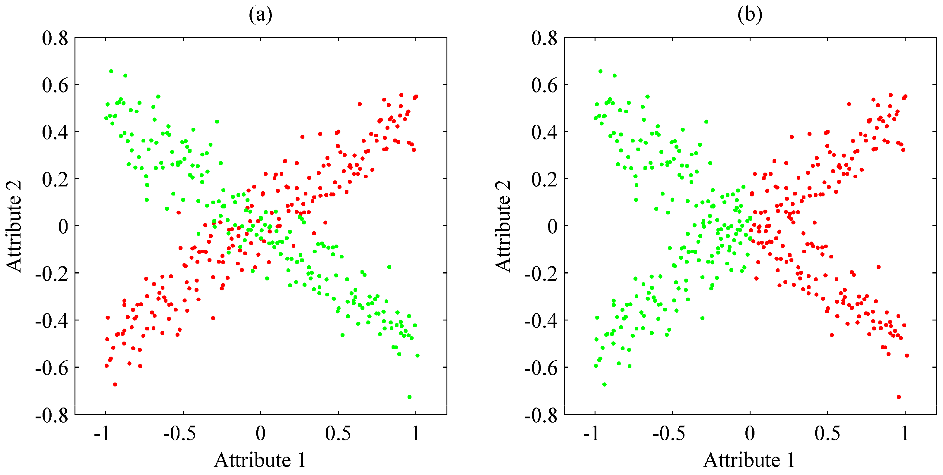
Figure 1. An example of the weakness of heuristic clustering methods. (a) Model-based methods such as Gaussian Mixture Model (GMM) can separate the two distinctive relationships of the two attributes, but (b) heuristic methods such as k-means clustering cannot.
Water 09 00723 g001
Figure 2. The study area. (a) Its location in the Heihe River Basin; (b) the groundwater sampling sites; and (c) the groundwater table and flow.
Water 09 00723 g002
Figure 3. The results of GMM clustering and k-means clustering in principal component (PC) spaces. (a) GMM, in PC1-PC2 space; (b) GMM, in PC2-PC3 space; (c) GMM, in PC1-PC3 space; (d) k-means, in PC1-PC2 space; (e) k-means, in PC2-PC3 space; (f) k-means, in PC1-PC3 space.
Water 09 00723 g003
Figure 4. The Piper diagram for the groundwater samples.
Water 09 00723 g004
Figure 5. Spatial patterns of the membership probabilities and the clustering uncertainty. (ae) the probabilities of the samples belonging to CLUSTERs 1 to 5, respectively, and (f) the clustering uncertainty.
Water 09 00723 g005
Figure 6. Spatial distributions of the clustered samples based on (a) GMM clustering; and (b) k-means clustering.
Water 09 00723 g006
Figure 7. Regionalization of the groundwater chemistry. Based on the GMM clustering, the study area can be divided into five sub-regions.
Water 09 00723 g007
Table 1. Correlation coefficient matrix of eight ions and TDS (log-transformed concentrations).
Na+K+Mg2+Ca2+ClSO42−NO3HCO3TDS
Na+1.0000.2520.7200.6110.9530.890−0.1090.4890.913
K+ 1.0000.5580.5050.2350.454−0.0120.4350.440
Mg2+ 1.0000.8910.6980.8870.1230.6570.905
Ca2+ 1.0000.5810.7860.0410.5710.815
Cl 1.0000.884−0.0740.4130.870
SO42− 1.000−0.0020.5950.959
NO3 1.0000.0190.015
HCO3 1.0000.718
TDS 1.000
Note: Coefficient values over 0.9 are in bold. The underlined numbers indicate insignificant correlations (p-value > 0.05).
Table 2. PCA loadings in different ions and variances explained by different PCs.
IonsPC1PC2PC3PC4
Na+0.402−0.2030.1600.411
K+0.3910.118−0.064−0.327
Mg2+0.4240.155−0.090−0.254
Ca2+0.3840.1800.031−0.478
Cl0.395−0.2020.1580.480
SO42−0.437−0.0490.0620.093
NO30.0600.768−0.4530.138
HCO3−0.0880.5050.8530.026
Variance explained61.5%14.4%11.5%7.5%
Cumulative variance explained61.5%75.8%87.3%94.8%
Table 3. Twelve candidate models and their associated likelihoods and BIC values.
Model IDKpAttributesLBIC
132PC1, PC2−177.74367.27
233PC1, PC2, PC3−187.02405.90
342PC1, PC2−169.92355.78
443PC1, PC2, PC3−119.71282.26
544PC1, PC2, PC3, PC4−143.77369.33
653PC1, PC2, PC3−87.12228.07
763PC1, PC2, PC3−65.09195.00
873PC1, PC2, PC3−78.33232.47
964PC1, PC2, PC3, PC4−146.6416.58
1043Cl, NO3, HCO3−111.787266.42
1133Cl, NO3, HCO3−158.52346.88
1237K+, Mg2+, Ca2+, Cl, NO3, HCO3, pH−535.411279
Table 4. Main characteristics of the five clusters with regard to salinity level and impacts of irrigation and fertilization.
ClusterSalinity Level (PC1 Score)Impact of Surface Water (PC2 Score)Impact of Fertilization (PC3 Score)Salinity Change Due to Recharge (PC1-PC2)Fertilization-Impacted Recharge (PC2-PC3)Groundwater Quality vs. Agricultural Development (PC1-PC3) *
CLUSTER 1Low to mediumMediumMediumEnhancedNoLimiting
CLUSTER 2Low to highLow to mediumLow to mediumInsignificantNoLimiting
CLUSTER 3LowMediumMediumInsignificantNoInsignificant
CLUSTER 4Medium to highMedium to highMedium to highEnhancedYesDegrading
CLUSTER 5Medium to highLowMedium to highReducedNoDegrading
Note: * “Limiting” refers to the effect that groundwater salinity limits the agricultural development. “Degrading” indicates the effect that fertilization enhances groundwater salinity.
Table 5. Spearman’s rank correlation coefficients between hydrological variables and membership probabilities *.
Hydrological Variablesm1m2m3m4m5
Potential ET−0.128−0.089−0.2700.0920.307
Groundwater ET−0.152−0.076−0.186−0.1910.282
Precipitation0.3160.0060.2570.268−0.184
Infiltration0.0950.010−0.1060.2353 × 10−4
Irrigation−0.0280.044−0.2840.157−0.140
Groundwater depth0.178−0.0310.4550.0270.214
UZ recharge−0.0840.004−0.1820.064−0.244
Note: * Coefficients with absolute values over 0.23 indicate significant correlation at the 95% confidence level and are bolded and underlined in the table.