Article

Climate Change Adaptation in a Mediterranean Semi-Arid Catchment: Testing Managed Aquifer Recharge and Increased Surface Reservoir Capacity

1
Water Research Institute, National Research Council, Headquarters of Rome, 00015 Rome, Italy
2
Water Research Institute, National Research Council, Branch of Brugherio, 20861 Brugherio, Italy
3
Water Research Institute, National Research Council, Branch of Bari, 70132 Bari, Italy
*
Author to whom correspondence should be addressed.
Water 2017, 9(9), 689; https://doi.org/10.3390/w9090689
Submission received: 7 August 2017 / Revised: 30 August 2017 / Accepted: 5 September 2017 / Published: 8 September 2017
(This article belongs to the Special Issue Adaptation Strategies to Climate Change Impacts on Water Resources)

Abstract

:
Among different uses of freshwater, irrigation is the most impacting groundwater resource, leading to water table depletion and possible seawater intrusion. The unbalance between the availability of water resources and demand is currently exacerbated and could become worse in the near future in accordance with climate change observations and scenarios provided by Intergovernmental Panel on Climate Change (IPCC). In this context, Increasing Maximum Capacity of the surface reservoir (IMC) and Managed Aquifer Recharge (MAR) are adaptation measures that have the potential to enhance water supply systems resiliency. In this paper, a multiple-users and multiple-resources-Water Supply System (WSS) model is implemented to evaluate the effectiveness of these two adaptation strategies in a context of overexploited groundwater under the RCP 4.5 and the RCP 8.5 IPCC scenarios. The presented a case study that is located in the Puglia, a semi-arid region of South Italy characterized by a conspicuous water demand for irrigation. We observed that, although no significant long-term trend affects the proposed precipitation scenarios, the expected temperature increase highly impacts the WSS resources due to the associated increase of water demand for irrigation purposes. Under the RCP 4.5 the MAR scenario results are more effective than the IMC during long term wet periods (typically 5 years) and successfully compensates the impact on the groundwater resources. Differently, under RCP 8.5, due to more persistent dry periods, both adaptation scenarios fail and groundwater resource become exposed to massive sea water intrusion during the second half of the century. We conclude that the MAR scenario is a suitable adaptation strategy to face the expected future changes in climate, although mitigation actions to reduce green-house gases are strongly required.

1. Introduction

Among the different uses of freshwater, irrigation is the most impacting of the groundwater resources [1], leading to water table depletion [2,3] and possible seawater intrusion (e.g., [4]). Water scarcity can be caused primarily by a shortage of available water, or an increasing demand [5]. Some authors (e,g., [2,6]) state that human interventions can affect groundwater more than climate drivers; at least, it is expected that direct human impacts could be of the same order of magnitude of a moderate global warming [3,6,7].
In many areas of the world, periodic water shortages, caused by temporal imbalances between supply and demand can be faced by storing water during rainy periods for later use during dry periods. The storage and recovery cycle could be seasonal or inter-year. In this regard, Mutiso [8] observed that in most arid and semiarid lands, the quest for water does not depend on the absolute amount of precipitation, but on the fraction retained.
The unbalance between the availability of water resources and demand is currently exacerbated and could become worse in the near future, by climate change, considering both the direct effects (i.e., increasing temperature and decreasing precipitation) and the secondary ones (i.e., increasing demand). Adaptation measures to water scarcity conditions can be built upon existing water management practices with the aim of increasing the resilience of water supply systems and decreasing their vulnerability to prolonged drought [5]. In a context of limited water availability in space and time, an integrated approach in the development and management of water resources is mandatory [9,10].
Among possible adaptation measures, the following are considered and compared in this paper as for this specific case study they appear to be the most feasible in the medium term: (1) an Maximum Capacity of the surface reservoir (IMC) (e.g., [11,12]) and (2) Managed Aquifer Recharge (MAR) (e.g., [13,14]). Artificial recharge systems are engineered systems where excess surface water (generally generated by floods on watersheds) is put on or in the ground for infiltration to aquifers to increase groundwater resource availability. In recent years [3,15,16], MAR has been proposed as one of the most effective adaptation measures in order to decrease the vulnerability of water supply systems in scarce conditions, especially in those areas where the impacts of climate change are more remarkable. The economic sustainability of this adaptation action has been recently demonstrated [17,18]. It is worth noting that the proposed adaptation scenarios do not take into account possible changes in the crop pattern, neither in time nor in space.
In this paper, we compare the effectiveness of two different adaptation strategies: increasing the surface water storage capacity and managed aquifer recharge. Their ability to cope with expected climate change under Representative Concentration Pathways RCP 4.5 and RCP 8.5 IPCC emission scenarios, to face the possible groundwater overexploitation in a multiple-users and multiple-resources water supply system has been assessed for a case study in Southern Italy, characterized by semi-arid Mediterranean climate and intensively irrigated agriculture.

2. Methods

The overall conceptual model is presented in Figure 1. The sub-model related to the water supply systems (impact model) was previously described in detail, calibrated, and validated in [19]. Expected climate change scenarios are represented by a coupled climate model, or Earth System Model (ESM), developed in the Coupled Model Intercomparison Project Phase 5 (CMPI5) [20] under the RCP 4.5 and RCP 8.5 [21,22]. Among possible RCP scenarios accounted for by the IPCC, they can be considered intermediate (RCP 4.5) and high (RCP 8.5) scenarios of future greenhouse gas concentration. Ground observations of monthly-cumulated precipitation and mean temperature are used to calibrate a statistical downscaling for each available ground station. A further spatial interpolation is computed over the ground station network for both observations and downscaled CMPI5 ESM historical and scenarios via kriging. The observed spatial autocorrelation among data has been assessed through the computation of the semi-variograms, and imposed by fitting them with a spherical model. Finally, the impact model [19] is forced by the resulting meteorological sets under different adaptation scenarios. The hindcast simulations resulting from the observed precipitation and temperature is used to assess the impact of the adaptation scenarios, while the RCP 4.5 and RCP 8.5 simulations investigate the interaction between climate change and the adaptation schemes. In the following, meteorological forcing, impact model, and adaptation scenarios are described.

2.1. Meteorological Forcing

In the framework of Figure 1, we built three spatially distributed meteorological forcing:
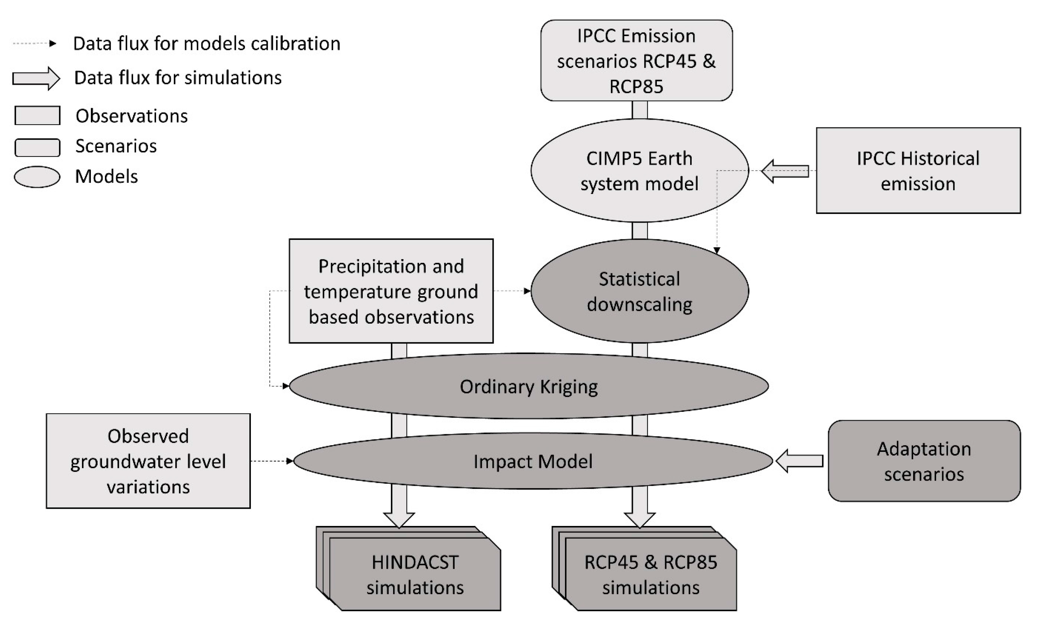
  • The Hindacst meteorological forcing has been obtained through the spatial interpolation of ground observation point measurements applying the ordinary kriging [23] to the monthly-observed precipitation and mean temperature. For precipitation, we found no evidence of altitude dependency or direction anisotropy. Thus, monthly spatial covariances were estimated through the experimental semi-variograms of precipitation for each month of the year. The ordinary kriging was then applied directly to the monthly-cumulated precipitation. Regarding temperature, a monthly lapse rate was calculated and the altitude dependency was removed before the estimation of monthly semi-variograms, after having verifyed that the resulting detrended temperature did not show any clear anisotropy. The ordinary kriging was then applied to the detrended temperature, and the observed lapse rate was applied to the resulting temperature.
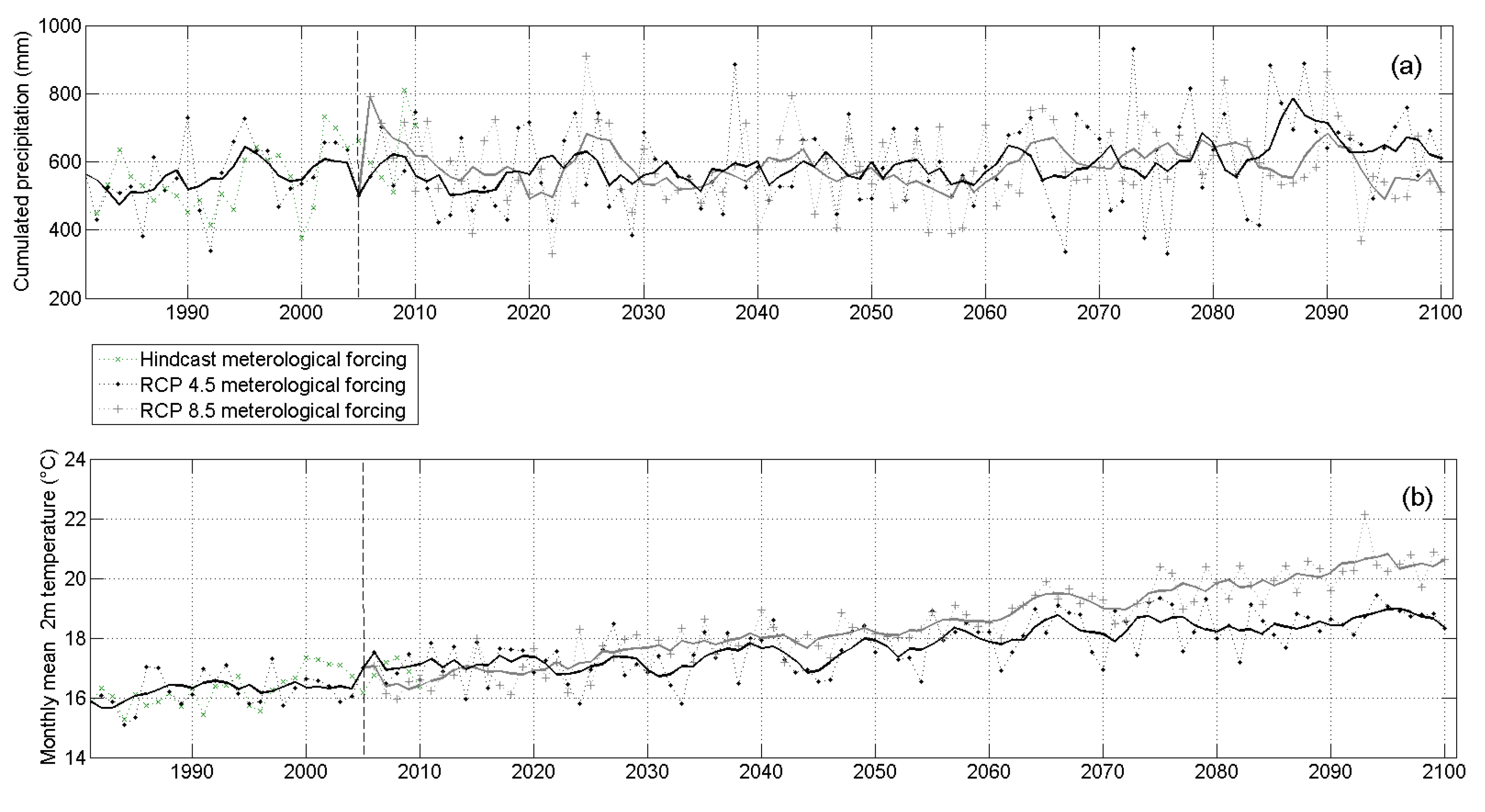
  • The historical RCP4.5 and RCP 8.5 meteorological forcing are represented by the CNRM-CM5 Earth system model (ESM). The CNRM-CM5 [24] consists of several existing models designed independently and coupled through the OASIS software developed at CERFACS: ARPEGE-Climate for the atmosphere, NEMO for the ocean, GELATO for sea-ice, SURFEX for land (ISBA scheme) and the ocean-atmospheric fluxes and TRIP to simulate river routing and water discharge from rivers to the ocean. The daily total precipitation and the daily mean temperature of all nodes covering and surrounding the case study have been extracted and aggregated at a monthly scale. To remove possible systematic bias, the resulting time series have been downscaled to the ground observation point measurements by applying a monthly quantile-quantile mapping correction technique [25]. Each station was compared with the nearest model node to build quantile-quantile mapping between the common period of the observations (predictor) and historical simulation (predictand) for each month of the year [26]. The predictand values lower and higher than the minimum and maximum observed quantiles have been linearly extrapolated. Finally, a spatial interpolation of point measurements (resulting from the historical, RCP4.5, and RCP8.5 meteorological forcing downscaled to the ground observation network) has been performed by applying the ordinary kriging method based on the semi-variograms of the observations fitted on the hindcast meteorological forcing.
In the following, time series built resulting from the aggregation of the historical and downscaled RCP 4.5 shall be referred as RCP 4.5 meteorological forcing. In the same way that the RCP 8.5 meteorological forcing has been built.

2.2. Impact Model

The overall impact model aims to reproduce the dynamic of a multiple-use and multiple-resource water schemes. It integrates the distributed the crop water requirements with surface and groundwater (GW) mass balance, considering the management rules of the current water supply system. The model is made up of four modules:
  • SPI-Q regression model: SPI-Q [27,28] is a multi-linear regression model simulating the monthly inflow to surface reservoir through a calibrated linear combination of Standardized Precipitation Indices (SPI, [29]) computed for different cumulative time scales of the precipitation data gathered in the area.
  • GMAT (Monthly Soil water balance): GMAT [30] is a distributed model that is able to simulate the soil water balance at a monthly scale for natural and agricultural land uses. Using the monthly precipitation and temperature time series, as well as the crops and soil features (all spatially distributed) as input, GMAT delivers the different components of the soil water balance (i.e., actual evapotranspiration, irrigation water demand, runoff, and groundwater recharge). The irrigation water demand is evaluated from the monthly soil water deficit only for irrigated crops.
  • Reservoir water balance model. The monthly water balance of the surface reservoir is computed accounting for the inflow estimated from the SPI-Q model, the irrigation water use estimated from the GMAT model, and the total amount of the other reservoir abstractions (e.g., human consumption, industrial uses, and environmental flows).
  • Aquifer water balance model. The monthly aquifer water balance is modelled as a lumped linear reservoir accounting for: (a) the groundwater recharge computed by GMAT; (b) the groundwater abstractions from private wells, computed assuming that the amount of the total demand for irrigation not supplied by the considered reservoir is supplied by the aquifer; and, (c) the groundwater outflow as discharge-to-sea and baseflow to the drainage network. Time variations in terms of actual total volume are delivered as output.
The implementation of the impact model is the same as described in detail in [19], with a slight modification in the reservoir model regulation rules: while in [19], the maximum storage capacity was considered constant in time, in the proposed study the maximum storage capacity is considered variable on a monthly base, according to the internal management rules imposing to leave part of the total volume available to flooding regulation. A short description of the main variables and associated nomenclature is given in Table 1.

2.3. Adaptation Scenarios

Three adaptation scenarios are considered under the Hindcast, RCP 4.5 and RCP 8.5 simulations:
  • Business as usual (BAU). The BAU scenario represents the current management rules of the water supply system.
  • Managed aquifer recharge (MAR). The MAR scenario proposes to take advantage of the current management rules for flooding control requiring keeping a minimum volume available in the case of heavy rainfall. In the proposed scenario, the controlled outflow operated from the irrigation pipelines (by opposition to uncontrolled overflow) is infiltrated to the GW through direct recharge, i.e., using the existing pumping wells as injection wells that can be feasibly connected to the irrigation network.
  • Increasing the maximum capacity of the surface reservoir (IMC). The IMC scenario proposes an increased maximum capacity of the surface reservoir. Such a scenario represents a widely recognized and straightforward vision of adaptation techniques (e.g., [31,32]). In practical terms, the increase of dam elevation is considered among the most effective in terms of increased volume per incremental unit of height. Further information concerning the implementation of the adaptation scenarios is given in Section 3.2.

3. Case Study

The study area (Figure 2) includes the irrigated areas of the Capitanata Plain (Puglia Region, South Italy), which is located within the administrative limits of the Province of Foggia, covering most of the alluvial plains of Puglia region, between the hilly area of the sub-Apennines to the South-West and the Gargano Plateau to the North-East. The area is one of the richest agricultural districts in Italy, covering an area of 4550 km2 with about 570,000 inhabitants; the area where the irrigation network is available covers approximately 1500 km2, but only 1260 km2 are effectively supplied. Two irrigation districts are established to serve about 40,000 delivery points: the Fortore district, in the Northern part, covering a surface area of 1100 km2, and the Sinistra Ofanto district, in the South, expanding over the surface area of 400 km2. Both districts are supplied by on-demand pressurized pipe networks and are equipped with water-meters at each user delivery point [33]. The “Consorzio per la Bonifica della Capitanata” (CBC) technical service is responsible for the overall planning and management of the two districts, including the operation of artificial reservoirs.
Due to its higher irrigation needs, the presented case study is focused on the Fortore district, which is mostly characterized by the combined use of both surface water coming from the Occhito dam and groundwater pumping operated at a farm-scale through more than 20,000 legal wells.
Concerning the capacity of the surface water supply, the mean annual withdrawal from the Occhito dam for the irrigation is about 95.9 Mm3, with a conveyance efficiency of 86.7% due to the operational losses and illegal water spills along the network [33].
The low ratio between the actually irrigated and the equipped area (around 46%) is partly due to the dominant cropping pattern, which is characterized by rainfed wheat (68% of the total land), followed by olive trees, tomato, vineyard, sugar beet, and vegetables [34]. Such a large difference is also connected to the extreme variability of inflows collected by the Occhito reservoir, which pushed farmers to withdraw water through private wells as a supplementary or alternative source for irrigation, leading to a depletion of the groundwater levels that eventually foster the sea water intrusion with a consequential degradation of the fresh water quality. Moreover, to face the endemic water scarcity, more efficient irrigation systems such as drip irrigation became widely spread (59%) as compared to the more water consuming sprinkler devices (27%) [35].
Under such conditions, which are all triggered by an increasing trend in the total irrigated area, it seems mandatory to undertake a quantitative estimation of the long-term sustainability of the conjunctive use of surface and ground water resources, particularly in view of possible climate changes. Therefore, besides studying measures to control irrigation water demand towards a more sustainable water balance [36], it seems reasonable also to investigate the feasibility of adaptation options seeking to increase the available water supply.

3.1. Parameterization of Models’ Components

Monthly rainfall and mean temperatures have been obtained from the regional hydro-climatic service covering a 35-year period from 1975 to 2010. The corresponding gauges network is shown in Figure 2. The ordinary kriging has been computed over a 1 km2 regular grid covering the whole case study. The combined process of statistical downscaling and spatial interpolation applied to CNRM-CM5 Earth system model results in a mean bias of −0.29 mm for monthly precipitation and 0.01 °C for monthly mean temperature, with respect to the hindcast meteorological forcing.
The initial aquifer volume and the linear GW coefficient k relating GW discharge to the water volume stored in the aquifer system have been calibrated through the observed water table variations resulting from three monitoring surveys carried out in 1987, 2002 to 2004, and 2007 to 2011 [37]. The monitoring wells are shown in Figure 2. The full parametrization and calibrations of the impact model is detailed in [19]. The monthly values of the maximum storage capacity (RWVmax) used in this study were provided by the land reclamation authority CBC based on the current managing rules for flood mitigation, and ranges between a minimum of 205.45 × 10⁶ m3 in winter and a maximum of 237.7 × 10⁶ m3 in summer. The range of maximum allowable retention volumes corresponds to storage elevations ranging from 192.0 and 194.3 m a.s.l. that are guaranteed through spillway operations equipped with Tainter gates to regulate spillway flow.
All the impact model parameters are reported in Table 2.

3.2. Parameterization of the Adaptation Scenarios

Managed aquifer recharge (MAR): This adaptation option aims at taking advantage of the flood control protocols with the possibility to infill the surface excess volumes to the GW. The controlled outflow is defined as the potential water volume exceeding the RWVmax of the current month, which is limited by the maximum control capacity of 250 × 106 m3. The water possibly exceeding the maximum control capacity (uncontrolled overflow) is not considered for managed aquifer recharge due to engineering and safety reasons. Moreover, the controlled outflow supplying the aquifer recharge system is limited by the maximum injection rate in existing wells that can potentially be connected to the current water distribution system (i.e., the existing wells located in the Reservoir Demand Area, Figure 2). The maximum injection rate of each well Qi has been estimated considering the recharge rates for vadose-zone wells in uniform soil material following from [5]:
Q i = K   2 π L 2 l n ( 2 L / r ) 1
where K is the hydraulic conductivity of the soil material, L is the water depth in the well, and r is the radius of the well. We estimated a mean monthly Qi of 2368 m3, considering a prudential value for the hydraulic conductivity of 10−6 m∙s−1, a mean water depth in the well of 25 m, and a mean radius of 0.25 m (average values according to available data). In the MAR scenario, we consider that 10,000 wells can be connected to the water supply system, which results in a monthly maximum injection capacity of GWR MAR max of 23.68 × 10⁶ m3. The monthly MAR water volume GWR MAR is computed as the product of the conveyance efficiency KCE and the controlled outflow is limited by the ratio of GWR MAR max by KCE. Finally, in the MAR scenario simulations, the reservoir overflow (RO) is recalculated as the sum of the uncontrolled and controlled outflow exceeding GWR MAR max / K CE .
Increasing maximum capacity of surface reservoir (IMC): In this case study, the scenario considers increasing the elevation of 2 m under the existing flood control rules. In practical terms, the range of the monthly maximum volumes (RWVmax, Table 2) and the maximum control capacity is increased by 28 × 106 m3 (corresponding to a maximum height increased from 195.15 to 197.1 m a.s.l.) adopting the same shape of the actual regulation rule.

4. Results and Discussions

4.1. Model Validation

The model validation has been performed over the hindcast run starting in 1981 with the full operation of the Occhito reservoir distribution network, in order to satisfy the hypothesis of the stationarity of the irrigation domain connected to the surface reservoir. The main model features can be reliably validated by considering the observed inflow to the reservoir, the actual irrigation water supplied to the CBC, the reservoir overflow, and the observed water volumes stored in the reservoir. The performance of the model can then be evaluated through its capacity to reproduce the hindcast BAU monthly variation of associated variables (i.e., inflow to reservoir, supplied water and stored volume, Figure 3). Guyennon et al., [19] provides more details on the model validation. Differently from the previous validation as discussed in [19], the implementation of the regulation rules for flooding mitigation slightly improves the overall model capacity in reproducing the observed reservoir volume variation and the irrigation demand supplied by the surface reservoir.

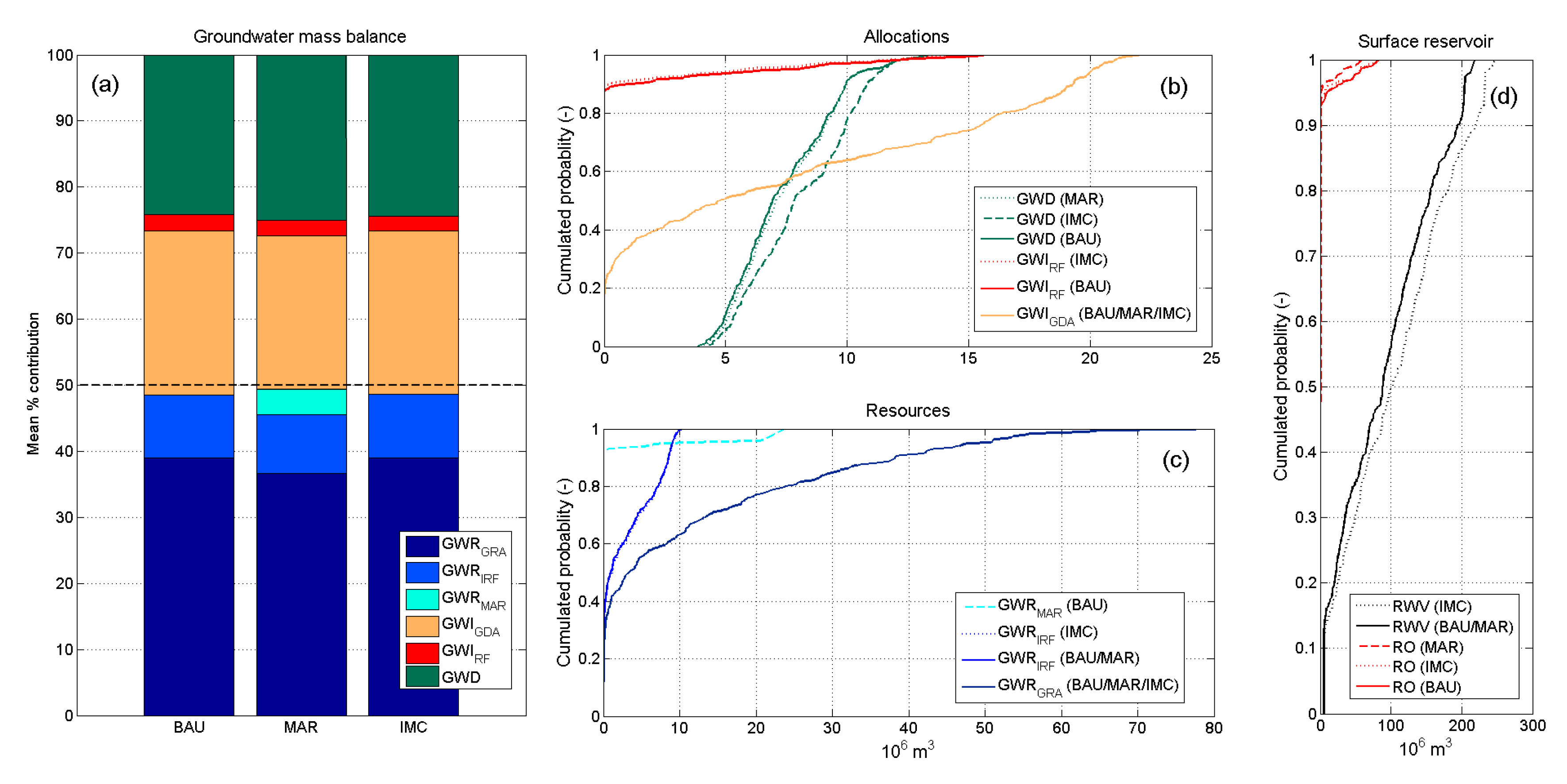
4.2. Expected Impact of Adaptation Scenarios

In order to investigate the expected impact of the proposed adaptation scenarios, independently from the expected climate change, the adaptation scenarios has been applied to the hindcast meteorological forcing since 1981 (full operation of the Occhito surface reservoir distribution network).
Figure 4a shows the impact of the MAR and IMC scenario as compared to the BAU in terms of GWV variation. The mean observed groundwater level variation since 1987 has been reported to the right axis. The MAR results are more efficient than the IMC scenario in increasing the GWV, but its impact is limited to the periods of weak winter North Atlantic Oscillation Index NAO (reported on a second right axis in Figure 4a), characterized by a higher precipitation in the proposed case study [19]. During long periods of strong winter NAO (middle 1990th, Figure 4a), the GWV drops back to the BAU levels; while during shorter dry periods (early and late 2000th), the gain of the MAR is less affected by the decreasing precipitation. The wet periods (indicatively middle 1980th, late 1990th to early 2000th, and late 2000th) are associated with an increasing occurrence of reservoir overflow (RO) (Figure 4b), corresponding to plurennial periods of high RWV levels (Figure 4c). During the hindcast period, the number of RO, and associated potential MAR volumes increased in both occurrence and magnitude (Figure 4b), resulting in a robust increase of GWV since the late 1990th with respect to the BAU. It is interesting to note that, with the proposed parametrization, the maximum monthly volume that can be actually filled in (as estimated in Section 3.2) limits the actual MAR volumes (Figure 4b). Differently, although the IMC scenario increases the RWV (Figure 4c) during periods of weak winter NAO, it does not succeed in increasing the surface reservoir levels during dry periods (i.e. early 1990 and early 2000), limiting the IMC capacity in reducing the groundwater extraction due to reservoir failure, and thus having a relative low impact on the GWV.
Results from Figure 4 indicate that, considering the past three decades, the MAR is a better option than the IMC as it takes advantage of the long term resiliency of the aquifer (typically 7 years resulting from the calibrated k, Table 2). On the contrary, the IMC is limited by the annual to plurennial response of the surface reservoir to the driest periods. Furthermore, the MAR is not able to cope with dry periods having duration similar to, or higher than, the long-term resiliency of the groundwater (as in 1990th).
To further investigate each component of the groundwater mass balance, the relative mean contribution (over the 1981–2010 period) of resources and allocations for each adaptation scenario is reported in Figure 5a. The resources are the natural recharge (GWRGRA), the recharge due irrigation return flow (GWRIRF), and the MAR recharge (GWRMAR). The allocations are the natural groundwater discharge (GWD), the direct groundwater extraction for irrigation (GWIGDA), and the groundwater extraction for irrigation associated to reservoir failure (GWIRF). By construction, the 50% line indicates equilibrium between resources and allocations. The associated mean absolute contributions are given in Table 3. Whereas, the associated quantile distributions are presented in Figure 5b,c for allocations and resources, respectively.
We can observe that when compared to the BAU and IMC, the MAR scenario reduces the relative impact of the GWIGDA, and the relative contribution of the GWRGRA to the overall groundwater mass balance (Figure 5a). It also increases the relative contribution of the GWD and drives the overall balance closer to the equilibrium. The GWRMAR represents 7.5% of the MAR groundwater resources (Table 3). Differently, the impact of the IMC scenario on the relative contribution of GWIRF is almost null when compared to the BAU (2.2% and 2.5%, respectively) (Figure 5a and Table 3).
The impact of adaptation scenarios on the allocation quantiles (Figure 5b) indicates that the increase of GWD due to the MAR is effective for all of the quantiles of the distribution. On the contrary, the IMC scenario affects only the lowest quantiles of GWIRF (Figure 5b), highly limiting its impact on the groundwater mass balance. This results from the fact that the impact of the IMC scenario on the RWV is effective for the higher quantiles (Figure 5d) but inefficient in increasing the lowest ones (associated with the surface reservoir failures). Finally, it is worth to note that the RO reduction is much more effective with the MAR scenario than with the IMC one (Figure 5d).

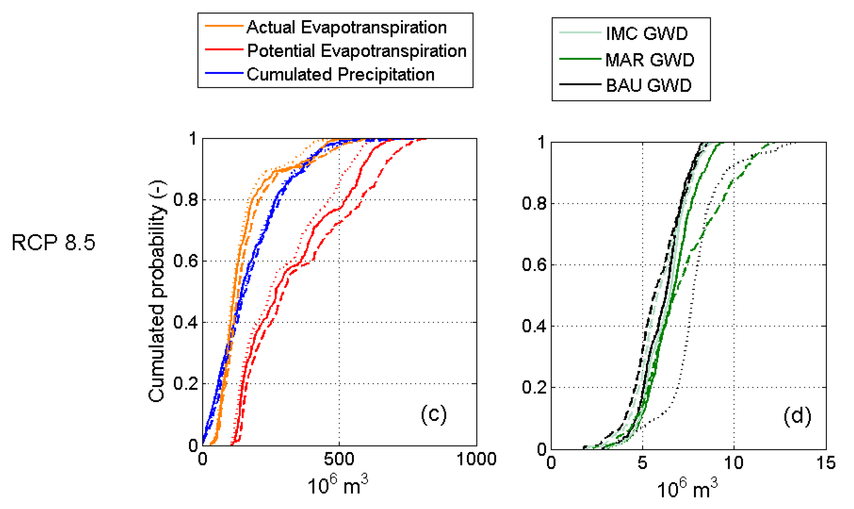
4.3. Managed Aquifer Recharge under Climate Change Scenarios

In order to investigate the interaction between expected climate change and the proposed adaptation scenarios, the impact model has been forced by the RCP 4.5 and RCP 8.5. Simulations begun in 1981 (full operation of the Occhito surface reservoir distribution network), and the adaptation scenarios (IMC and MAR) start in 2020.
Figure 6 presents, for both meteorological scenarios and for the hindcast, the mean annual cumulated precipitation (panel a) and the mean annual mean temperature (panel b) over the case study. A 5-years moving average has been added for the RCP 4.5 and RCP 8.5 meteorological, forcing to highlight the long-term variability.
When compared with the hindcast, the selected ESM success in reproducing the observed precipitation inter annual and decadal variability (Figure 6a), with a significant long term positive autocorrelation ranging from 68 to 82 months for hindcast, from 70 to 81 months for RCP 4.5 and from 69 to 81 months for RCP 8.5 over their common period.
The Mann Kendall test [40] has been performed on the annual precipitation and temperature time series to test possible for significant increasing/decreasing trends. The Mann Kendall test indicates that both the RCP 4.5 and RCP 8.5 annual precipitation did not present a significant trend (p > 0.01) over the 2006–2100 period. On the contrary, the mean temperature presents a significant (p < 0.001) positive trend for both RCP 4.5 and RCP 8.5 (+0.021 °C∙year–1 and +0.045 °C∙year−1 over the 2006–2100 period, respectively, Figure 6b). It is worth to note that during the first half of the 21st century, both scenarios present similar temperature values, but differ during the second half.
Figure 7 shows the results of the impact models forced by RCP 4.5 and RCP 8.5 (referred as RCP 4.5 and RCP 8.5 simulations in the following) for the BAU, MAR, and IMC adaptation scenarios. In order to assess the impact of the long-term variation in the precipitation, the five-year (60 months) standard precipitation index (SPI) has been reported together with the BAU, MAR, and IMC groundwater volumes (GWV). The hindcast GWV under BAU scenario has also been reported for a qualitative comparison with the RCP 4.5 and RCP 8.5 simulations.
The RCP 4.5 and RCP 8.5 confirm that the MAR adaptation scenario is more effective than the IMC in taking advantage of plurennial positive SPI. Similar to the MAR hindcast simulation (Figure 4), the GWV under the MAR scenario increases during wet periods (as indicated by the positive long-term SPI), independently from the emission scenario (Figure 7a,b), but drops down during long dry periods (indicated by the negative long-term SPI) to level similar to the BAU scenarios.
Independently from the adaptation scenario, both RCP 4.5 and RCP 8.5 simulations present a similar impact on the groundwater volumes during the first half of the 21th century. Differently, during the second half, the RCP4.5 GWV significantly increases thanks to the MAR adaptation (Figure 7a), while for the RCP 8.5 scenario, the groundwater volume drops down under levels exposing the coastal aquifer to sea-water intrusion (Figure 7b). In this case, neither the IMC nor MAR scenarios are able to mitigate possible sea-water intrusion.
It clearly appears that the periods of increase of groundwater levels correspond to sequences of plurennial relative high levels in the surface reservoir (Figure 7e,f). These periods results in an increased occurrence of RO events (Figure 7c,d), from which the MAR adaptation scenarios can take advantage to increase the GWV (Figure 7a,b). On the contrary, the major decrease in the GWV occurs during plurennial low levels in the surface reservoir. These periods are associated with a persisting negative long-term SPI. If the negative trend in the RCP 8.5 GWV is not associated to a significant negative trend in precipitation, but rather to a positive trend in mean temperature (Figure 6), and associated significant increase in the total water demand for irrigation (+0.13 and +0.58 106 m3∙year−1 for RCP 4.5 and RCP 8.5, respectively), the extent of the plurennial variability in the precipitation and resulting duration of the dry periods has the major impact on the GWV, as occurs for the RCP 8.5 during the 2030th and the 2050th.
To further investigate the dynamics of the water supply system for each adaptation scenarios and meteorological forcing, the mean contribution of each component of the groundwater mass balance, the RO, the GWV, and RWV for the periods 1981–2020, 2021–2060, and 2061–2100 are given in Table 4. Their associated relative impact to the mass balance is reported in Figure 8. The expected impact of climate change on the groundwater mass balance and its interactions with the water supply system results in an increase of the relative contribution of the direct abstraction for irrigation (GWIGDA), and a decrease of the groundwater natural discharge (GWD) (Figure 8). The relative contribution of the natural recharge (GWRGRA), the recharge due to irrigation return flow (GWRIRF), and the groundwater abstraction to face the surface reservoir failure (GWIRF) remain mostly stable (Figure 8). The IMC adaptation successfully increases the long term mean water volume of the surface reservoir (Table 4), but the associated reduction in of the groundwater abstraction to face the surface reservoir failure (GWIRF) is limited (Figure 8 and Table 4). Differently, the capacity of the MAR scenario to take advantage of plurennial positive SPI to increase groundwater levels (Figure 4 and Figure 7) during the wet periods increase the long term (40 years) mean contribution of the natural groundwater discharge (Figure 8, Table 4) to the overall aquifer budget.
Independently from the adaptation scenario, the long-term (40 years) mean contribution is negatively unbalanced for both of the emission scenarios during the 1981–2020 period, and for RCP 8.5 during the 2021–2060 period, while its results are almost balanced during the 2061–2100 period of the century for both RCP (Figure 8). Differently, the groundwater discharge (GWD) continuously decreases for both of the RCP scenarios (Table 4). Considering that the highest values in the long term precipitation significant autocorrelation are observed for the RCP 8.5 2021–2060 period, such a result confirms that the variation in the long-term dry periods has a major impact on the groundwater balance and the resulting GWV with respect to the increased irrigation water demand. This is due to higher temperature, which rather reduces the associated GWD, keeping the groundwater balanced.
The dynamic system resulting from the interactions between climate, irrigated agriculture and associated water supply systems, soil moisture, and groundwater dynamics is a complex low pass filter combining seasonal (soil moisture), pluri-annual (surface reservoir), and decadal (groundwater and natural precipitation long term oscillations) time scales. From the perspective of the sustainability of the irrigated agriculture, and thus the possible aquifer overexploitation, the dynamic system can be simplified to the nonlinear transfer function between the climate forcing and the groundwater natural discharge. Figure 9 presents the cumulated density function of cumulated precipitation (Rt), potential, and actual evapotranspiration (ETP and ETR), and the natural groundwater discharge (GWD) for the periods 1981–2020 (dot lines), 2021–2060 (full lines), and 2061–2100 (dash lines). The expected climate change affects a wide range of the quantiles of the potential evapotranspiration (cdf > 0.4 and cdf > 0.2 for RCP 4.5 and RCP 8.5, respectively), and only the highest quantiles of the RCP 4.5 monthly cumulated precipitation (cdf > 0.8) (Figure 9a,c). The resulting interactions with the irrigation water supply system through the soil moisture dynamic increases the highest and upper quantiles of the actual evapotranspiration (ETR) for the RCP 4.5 and RCP8.5, respectively (cdf > 0.8 and cdf > 0.6) (Figure 9a,c). The resulting impact on the GWD affects the whole quantile distribution with a systematic reduction of the discharge to the sea, except for the MAR scenario during the 2021–2060 period with an increase for cdf > 0.7 and <0.9 (Figure 9b,d) when compared with the 1980–2020 period.

5. Conclusions

We observed that in the Puglia Region the groundwater volume present natural fluctuations at a typical decadal time scale associated with winter NAO, but it results were negatively affected by the water demand for irrigation associates to soil moisture dynamics [19]. We were able to examine the impact of two adaptation scenarios under expected climate change scenarios (1980–2100 period): the increase surface reservoir maximum capacity (IMC) and a managed aquifer recharge (MAR) taking advantage of the managed overflow for flood control purpose. The MAR scenario was observed as more effective than the IMC one during the wet periods (typically 5 years) in increasing the groundwater resource (GWV). However, both of the cases show that the GWV tends to drop down to business as usual (BAU) levels during dry periods (typically 5 years). If no significant trend affects the proposed precipitation scenarios (CMPI5 CNRM-CM5 under RCP 4.5, and RCP 8.5 IPCC scenarios), the expected increase in temperature highly impacts the water supply system due to the associated increased demand for irrigated agriculture, reducing the groundwater natural discharge. In this context, the MAR scenario results in effective in mitigating of the impact of the increased temperature on the long-term (40 years) groundwater discharge (and associated ecosystem services) under RCP 4.5. Under RCP 8.5, the groundwater drops down due to more persistent dry periods (despite the lack of significant negative trend in the precipitation) and is exposed to massive saline water intrusion during the second half of the century, independently from the adaptation scenario.
The present results illustrate the need for a combined effort in both global mitigation (RCP scenarios) and local adaptation actions (adaptation scenarios) to preserve the regional water resource for the next generations.

Author Contributions

N. Guyennon, I. Portoghese, E. Romano and F. Salerno conceived and designed the numerical experiments; N. Guyennon performed the numerical experiments; N. Guyennon, E. Romano and I. Portoghese analyzed the data; N. Guyennon, F. Salerno, E. Romano and I. Portoghese wrote the paper.

Conflicts of Interest

The authors declare no conflict of interest.

References

  1. Shiklomanov, I.A.; Rodda, J.C. World Water Resources at the Beginning of the 21st Century; Cambridge University Press: Cambridge, UK, 2003. [Google Scholar]
  2. Green, T.R.; Taniguchi, M.; Kooi, H.; Gurdak, J.J.; Allen, D.M.; Hiscock, K.M.; Treidel, H.; Aureli, A. Beneath the surface of global change: Impacts of climate change on groundwater. J. Hydrol. 2011, 405, 532–560. [Google Scholar] [CrossRef]
  3. Taylor, R.G.; Scanlon, B.; Döll, P.; Rodell, M.; Van Beek, R.; Wada, Y.; Longuevergne, L.; Leblanc, M.; Famiglietti, J.S.; Edmunds, M.; et al. Ground water and climate change. Nat. Clim. Chang. 2013, 3, 322–329. [Google Scholar] [CrossRef] [Green Version]
  4. Zaccaria, D.; Passarella, G.; D’Agostino, D.; Giordano, R.; Solis, S.S. Risk Assessment of Aquifer Salinization in a Large-Scale Coastal Irrigation Scheme, Italy. CLEAN—Soil, Air, Water 2016, 44, 371–382. [Google Scholar] [CrossRef]
  5. Bouwer, H. Artificial recharge of groundwater: Hydrogeology and engineering. Hydrogeol. J. 2002, 10, 121–142. [Google Scholar] [CrossRef]
  6. Haddeland, I.; Heinke, J.; Biemans, H.; Eisner, S.; Flörke, M.; Hanasaki, N.; Wisser, D. Global water resources affected by human interventions and climate change. Proc. Natl Acad. Sci. USA 2014, 111, 3251–3256. [Google Scholar] [CrossRef] [PubMed]
  7. Falloon, P.; Betts, R. Climate impacts on European agriculture and water management in the context of adaptation and mitigation—The importance of an integrated approach. Sci. Total Environ. 2010, 408, 5667–5687. [Google Scholar] [CrossRef] [PubMed]
  8. Mutiso, S. The significance of subsurface water storage in Kenya. In Management of Aquifer Recharge and Subsurface Storage; Tuinhof, A., Heederik, J.P., Eds.; (NNC-IAH) Publication No. 4; Netherlands National Committee—International Association of Hydrogeologists: Wageningen, The Netherlands, 2003; pp. 25–31. [Google Scholar]
  9. Preziosi, E.; Del Bon, A.; Romano, E.; Petrangeli, A.B. Vulnerability to Drought of a Complex Water Supply System. The Upper Tiber Basin Case Study (Central Italy). Water Resour. Manag. 2013, 27, 4655–4678. [Google Scholar] [CrossRef]
  10. Sobowale, A.; Ramalan, A.A.; Mudiare, O.J.; Oyebode, M.A. Groundwater recharge studies in irrigated lands in Nigeria: Implications for basin sustainability. Sustain. Water Qual. Ecol. 2014, 3, 124–132. [Google Scholar] [CrossRef]
  11. Bates, B.C.; Kundzewicz, Z.W.; Wu, S.; Palutikof, J.P. Climate Change Water; Bryson, C.B., Zbigniew, W.K., Wu, S., Jean, P., Eds.; IPCC Secretariat: Geneva, Switzerland, 2008. [Google Scholar]
  12. Boelee, E.; Mekonnen, Y.; Poda, J.N.; McCartney, M.; Cecchi, P.; Kibret, S.; Hagos, F.; Laamrani, H. Options for water storage and rainwater harvesting to improve health and resilience against climate change in Africa. Reg. Environ. Chang. 2013, 13, 509–519. [Google Scholar] [CrossRef]
  13. Sprenger, C.; Hartog, N.; Hernández, M.; Vilanova, E.; Grützmacher, G.; Scheibler, F.; Hannappel, S. Inventory of managed aquifer recharge sites in Europe: Historical development, current situation and perspectives. Hydrogeol. J. 2017, 25, 1–14. [Google Scholar] [CrossRef]
  14. Masciopinto, C.; Vurro, M.; Palmisano, V.N.; Liso, I.S. A Suitable Tool for Sustainable Groundwater Management. Water Resour. Manag. 2017, 1–15. [Google Scholar] [CrossRef]
  15. Megdal, S.B.; Dillon, P.; Seasholes, K. Water Banks: Using Managed Aquifer Recharge to Meet Water Policy Objectives. Water 2014, 6, 1500–1514. [Google Scholar] [CrossRef]
  16. Megdal, S.B.; Dillon, P. Policy and Economics of Managed Aquifer Recharge and Water Banking. Water 2015, 7, 592–598. [Google Scholar] [CrossRef]
  17. Maliva, R.G. Economics of Managed Aquifer Recharge. Water 2016, 6, 1257–1279. [Google Scholar] [CrossRef]
  18. Damigos, D.; Tentes, G.; Balzarini, M.; Furlanis, F.; Vianello, A. Revealing the economic value of Managed Aquifer Recharge: Evidence from a Contingent Valuation study in Italy. Water Resour. Res. 2017, 53, 1–15. [Google Scholar] [CrossRef]
  19. Guyennon, N.; Romano, E.; Portoghese, I. Long-term climate sensitivity of an integrated water supply system: The role of irrigation. Sci. Total Environ. 2016, 565, 68–81. [Google Scholar] [CrossRef] [PubMed]
  20. Taylor, K.E.; Stouffer, R.J.; Meehl, G.A. An overview of CMIP5 and the experiment design. Bull. Am. Meteorol. Soc. 2012, 93, 485–498. [Google Scholar] [CrossRef]
  21. Moss, R.; Babiker, W.; Brinkman, S.; Calvo, E.; Carter, T.; Edmonds, J.; Elgizouli, I.; Emori, S.; Erda, L.; Hibbard, K.; et al. Towards New Scenarios for the Analysis of Emissions: Climate Change, Impacts and Response Strategies; IPCC Secretariat: Geneva, Switzerland, 2007; ISBN 9789291691241. [Google Scholar]
  22. Moss, R.H.; Edmonds, J.A.; Hibbard, K.A.; Manning, M.R.; Rose, S.K.; Van Vuuren, D.P.; Carter, T.R.; Emori, S.; Kainuma, M.; Kram, T.; et al. The next generation of scenarios for climate change research and assessment. Nature 2010, 463, 747–756. [Google Scholar] [CrossRef] [PubMed]
  23. Cressie, N. Spatial prediction and ordinary kriging. Math. Geol. 1988, 20, 405–421. [Google Scholar] [CrossRef]
  24. Voldoire, A.; Sanchez-Gomez, E.; Salas y Mélia, D.; Decharme, B.; Cassou, C.; Sénési, S.; Valcke, S.; Beau, I.; Alias, A.; Chevallier, M.; et al. The CNRM-CM5.1 global climate model: Description and basic evaluation. Clim. Dyn. 2013, 40, 2091–2121. [Google Scholar] [CrossRef] [Green Version]
  25. Déqué, M. Frequency of precipitation and temperature extremes over France in an anthropogenic scenario: Model results and statistical correction according to observed values. Glob. Planet. Chang. 2007, 57, 16–26. [Google Scholar] [CrossRef]
  26. Guyennon, N.; Romano, E.; Portoghese, I.; Salerno, F.; Calmanti, S.; Petrangeli, A.B.; Tartari, G.; Copetti, D. Benefits from using combined dynamical-statistical downscaling approaches-lessons from a case study in the Mediterranean region. Hydrol. Earth Syst. Sci. 2013, 17, 705. [Google Scholar] [CrossRef]
  27. Romano, E.; Del Bon, A.; Petrangeli, A.B.; Preziosi, E. Generating synthetic time series of springs discharge in relation to standardized precipitation indices. Case study in Central Italy. J. Hydrol. 2013, 507, 86–99. [Google Scholar] [CrossRef]
  28. Romano, E.; Guyennon, N.; Del Bon, A.; Petrangeli, A.B.; Preziosi, E. Robust method to quantify the risk of shortage for water supply systems. J. Hydrol. Eng. 2017, 22, 04017021. [Google Scholar] [CrossRef]
  29. McKee, T.B.; Doesken, N.J.; Kleist, J. The relationship of drought frequency and duration to time scales. In Proceedings of the 8th Conference on Applied Climatology, Anaheim, CA, USA, 17–22 January 1993. [Google Scholar]
  30. Portoghese, I.; Uricchio, V.; Vurro, M. A GIS tool for hydrogeological water balance evaluation on a regional scale in semi-arid environments. Comput Geosci. 2005, 31, 15–27. [Google Scholar] [CrossRef]
  31. Milly, P.C.; Betancourt, D.J.; Falkenmark, M.; Hirsch, R.M.; Kundzewicz, Z.W.; Lettenmaier, D.P.; Stouffer, R.J. Stationarity is dead: Whither water management? Science 2008, 319, 573–574. [Google Scholar] [CrossRef] [PubMed]
  32. Taylor, R. Rethinking Water Scarcity: The Role of Storage. Eos 2009, 90, 237–238. [Google Scholar] [CrossRef]
  33. Lamaddalena, N.; D’Arcangelo, G.; Billi, A.; Todorovic, M.; Hamdy, A.; Bogliotti, C.; Quarto, A. Participatory water management in Italy: Case study of the Consortium “Bonifica della Capitanata”. Opt. Méditer. Ser. B 2004, 48, 159–169. [Google Scholar]
  34. Istituto Nazionale di Economia Agraria (INEA). Information System for Water Management in Agriculture (SIGRIA), INEA Rome, 2000. Available online: http://inea.it/irri/carte.cfm (accessed on 23 October 2008). (In Italian).
  35. ISTAT, Istituto Nazionale di Statistica. 5° National Agricultural Census, Istat Roma, 2000. Available online: http://censagr.istat.it/ (accessed on 10 November 2015). (In Italian).
  36. Zingaro, D.; Portoghese, I.; Giannocaro, G. Modelling crop pattern change and water resources exploitation: A case study. Water. Under review. [CrossRef]
  37. Passarella, G.; Barca, E.; Sollitto, D.; Masciale, R.; Bruno, D.E. Cross-Calibration of Two Independent Groundwater Balance Models and Evaluation of Unknown Terms: The Case of the Shallow Aquifer of “Tavoliere di Puglia” (South Italy). Water Resour. Manag. 2017, 31, 327–340. [Google Scholar] [CrossRef]
  38. Ciollaro, G.; Lamaddalena, N.; Altieri, S. Analisi comparativa fra consumi idrici stimati e misurati in un distretto irriguo dell’Itala meridionale [Comparative analysis between estimated and measured water needs in an irrigated district of Southern Italy]. Associazione Italiana di Genio Rurale—Rivista di Ingegneria Agraria 1993, 4, 234–243. (In Italian) [Google Scholar]
  39. Todorovic, M.; Lamaddalena, N.; Liuzzi, G.T. Modern Strategies and Tools for Water Saving and Drought Mitigation in Southern Italy; The International Centre for Advanced Mediterranean Agronomic Studies: Zaragoza, Spain, 2008. [Google Scholar]
  40. Kendall, M.G. Rank Correlation Methods; Oxford University Press: New York, NY, USA, 1975. [Google Scholar]
Figure 1. Block diagram of the overall conceptual model. Dash black arrows indicates data flux for calibration. Wide gray arrow indicates data flux for simulations. Dark blocks indicate steps implemented in this research.
Water 09 00689 g001
Figure 2. Case study. Upper panels: case study localizations. Center and Lower panels: groundwater recharge and demand areas as defined in Section 2. The Occhito reservoir, as well as, the considered unconfined/confined aquifer domains [37] are shown on each panel, while precipitation and temperature gauges are shown only in the reservoir demand area panel for a better visualization. Monitoring wells are shown in the groundwater demand area (refer to [19]).
Water 09 00689 g002
Figure 3. Model validation. Panel (a): observed and simulated inflow to reservoir. Panel (b): scatter plot and monthly correlation of observed and simulated inflow to reservoir (in legend). Panel (c): observed and simulated water consumption. Panel (d): scatter plot and monthly correlation of observed and simulated water consumption (in legend). Panel (e): observed and simulated stored water volume and overflow (full lines and stems respectively). Panel (f): scatter plot and monthly correlation of observed and simulated stored water volume and overflow (in legend).
Water 09 00689 g003
Figure 4. Panel (a): expected impact of adaptation scenarios on the groundwater available volume and observed groundwater level variation with associated spatial variability (error bar) (right axes). The Winter North Atlantic Oscillation and associated 5 years smoothing are reported on a second right axis. Panel (b): total overflow from the surface reservoir, potential overflow available for the aquifer recharge and actual volume infiltrated for the MAR Hindcast simulation. Panel (c): surface reservoir available volume for the BAU and IMC scenarios.
Water 09 00689 g004
Figure 5. Panel (a): absolute percentage contribution to the aquifer mass balance for each scenario. Natural recharge to aquifer (GWRGRA), recharge due to irrigation return flow (GWRIRF) and managed aquifer recharge (GWRMAR), direct abstraction from the aquifer (GWIGDA), abstraction due to surface reservoir shortage (GWIRF), and discharge to sea are (GWD). By construction, the 50% line indicates equilibrium between Resources (cold colors) and Allocations (hot and green colors) components. Panel (b) cumulated density function of allocations for each adaptation scenario. Panel (c): cumulated density function of resources for each adaptation scenario. Panel (d): cumulated density function of the Occhito surface reservoir volume (RWV) and overflow (RO).
Water 09 00689 g005
Figure 6. Panel (a): annual cumulated precipitation for the Hindcast (green dash line), RCP 4.5 (black dot line) and RCP 8.5 (gray dot line) meteorological forcing. Associated 5 years smoothing for RCP 4.5 (black full line) and RCP 8.5 (grey full line) meteorological forcing. The vertical dash line indicates the end of the common historical period. Panel (b) annual mean temperature (same layout).
Water 09 00689 g006
Figure 7. Panels (a): expected impact on the groundwater available volume of adaptation scenarios starting in 2020 under RCP 4.5. The associated 60 month (5 years) SPI is reported on the right axes. Panel (b): expected impact on the groundwater available volume of adaptation scenarios starting in 2020 under RCP 8.5. The associated 60 month (5 years) SPI is reported on the right axes. Panels (c) and associated total overflow from the surface reservoir, and actual volume infiltrated for the managed aquifer recharge (MAR) under RCP 4.5. Panel (d): associated total overflow from the surface reservoir, and actual volume infiltrated for the managed aquifer recharge (MAR) under RCP 8.5. Panel (e): surface reservoir available volume under RCP 4.5. Panel (f): surface reservoir available volume under RCP 8.5. The vertical dash lines indicate the starting year of adaptation scenarios. The vertical dot lines indicate the beginning of RCP 4.5 (panels a, c and e) and RCP 8.5 (panels b, d and f) emission scenarios.
Water 09 00689 g007
Figure 8. Top panels: percentage contribution to aquifer mass balance within each adaptation scenario (starting in 2020) under the RCP 4.5 emission scenarios for the periods 1981–2020 (top-right panel), 2021–2060 (top-middle panel) and 2061–2100 (top-left panel) from (same layout of Figure 4a). Lower panels: same analysis under the RCP 8.5 emission scenarios. By construction, the 50% line indicates equilibrium between the Resources (cold colors) and Allocations (hot and green colors) components.
Water 09 00689 g008
Figure 9. Panel (a): cumulated density function of monthly cumulated precipitation, potential and actual evapotranspiration of the RCP 4.5 simulations for the periods 1981–2020 (dot lines), 2021–2060 (full lines) and 2061–2100 (dash lines). Panel (b): cumulated density function of natural groundwater discharge (GWD) (same layout of panel a). Panels (c): results of RCP 8.5 simulations (same layout of panel a). Panels (d): results of RCP 8.5 simulations (same layout of panel b).
Water 09 00689 g009aWater 09 00689 g009b
Table 1. Short description and nomenclature of meteorological forcings and impact model variables considered for this case study and described in details in [19].
ModelVariableUnitDescription
Meteorological forcingETPmm [month]Distributed potential evapotranspiration
Ta°CDistributed monthly mean of daily mean temperature at 2 m
Rtmm [month]Distributed monthly cumulated precipitation
Domain definitionsGRAm2Groundwater recharge area
RDAm2Reservoir demand area: area connected to the surface reservoir distribution network
GDAm2Groundwater demand area: entire domain except the RDA
GMAT modelETRmm [month]Distributed actual evapotranspiration
GWRmm [month]Distributed groundwater recharge
GWIm3 [month]Distributed Groundwater extraction
Reservoir water balance modelRWVm3 [month]Surface reservoir water volume
ROm3 [month]Surface reservoir overflow
GWIRFm3 [month]Groundwater abstractions needed for irrigation in case of reservoir failure
Aquifer Water Balance ModelGWRGRAm3 [month]Groundwater recharge cumulated over the groundwater recharge area
GWRIRFm3 [month]Cumulated recharge to aquifer due to the irrigation return flow
GWDm3 [month]Cumulated Natural groundwater outflow as discharge to the sea and river baseflow
GWIGDAm3 [month]Cumulated direct abstraction to groundwater for irrigation
GWVm3 [month]Groundwater volume
Table 2. Impact model parameterization.
VariableUnitValueDescriptionSource
KGDI-0.70Deficit irrigation coefficient[38]
KCE-0.87Mean conveyance efficiency[39]
KIE-0.70Mean irrigation efficiency[39]
kMonth−10.0116Groundwater outflow linear rate coefficient[19]
GWVinit106 m31100Initial groundwater volume [19]
RWVmax106 m3[205.45, 237.7]Range of maximum storage capacityCBC
Table 3. Annual cumulated mean water volume (Mm3) of each term of the groundwater mass balance (GWRGRA, GWRIRF, GWRMAR, GWIGDA, GWIRF and GWD) and for the reservoir total overflow (RO) and mean water volume (106 m3) for the surface reservoir (RWV) and the groundwater (GWV) for each hindcast scenario over the period 1981–2010.
Groundwater Mass Balance TermHindcast 1981–2010
BAUMARIMC
GWRGRA143.5143.5143.5
GWRIRF34.834.835.6
GWRMAR0.014.60.0
GWIGDA−91.1−91.1−91.1
GWIRF−9.4−9.4−8.2
GWD−88.7−97.7−90.0
Table 4. Annual cumulated mean water volume (106 m3) of each term of the groundwater mass balance (GWRGRA, GWRIRF, GWRMAR, GWIGDA, GWIRF and GWD) and for the reservoir total overflow (RO) and mean water volume (106 m3) for the surface reservoir (RWV), and the groundwater (GWV) for each RCP 4.5 and RCP 8.5 scenarios over the periods 1981–2020, 2021–2060 and 2061–2100.
Mass Balance TermsRCP 4.5
1981–20202021–20602061–2100
BAU BAUMARIMCBAUMARIMC
GWRGRA138.5 136.4136.4136.4142.8142.8142.8
GWRIRF39.8 39.239.240.039.339.340.1
GWRMAR0.0 0.05.30.00.020.00.0
GWIGDA−95.3 −97.1−97.1−97.1−98.4−98.4−98.4
GWIRF−5.5 −7.5−7.5−6.3−7.8−7.8−6.4
GWD−93.6 −73.5−79.0−75.5−69.4−85.9−71.5
RO12.2 8.62.56.336.713.733.6
RWV105.0 85.485.4100.4106.0106.0122.7
GWV664.3 521.7560.9535.8492.6610.1507.8
Mass Balance TermsRCP 8.5
1981–20202021–20602061–2100
BAU BAUMARIMCBAUMARIMC
GWRGRA143.5 126.7126.7126.7123.0123.0123.0
GWRIRF38.4 36.436.436.839.739.740.5
GWRMAR0.0 0.05.80.00.011.50.0
GWIGDA−90.0 −99.0−99.0−99.0−108.2−108.2−108.2
GWIRF−3.8 −13.6−13.6−13.0−13.9−13.9−12.7
GWD−101.5 −58.8−64.3−60.4−44.0−54.6−45.7
RO27.6 10.84.19.418.65.415.8
RWV115.8 72.972.978.579.079.089.9
GWV720.4 417.6456.8428.9312.2387.7324.6

