
CryoSat-2 Altimetry Applications over Rivers and Lakes


Abstract
:1. Introduction
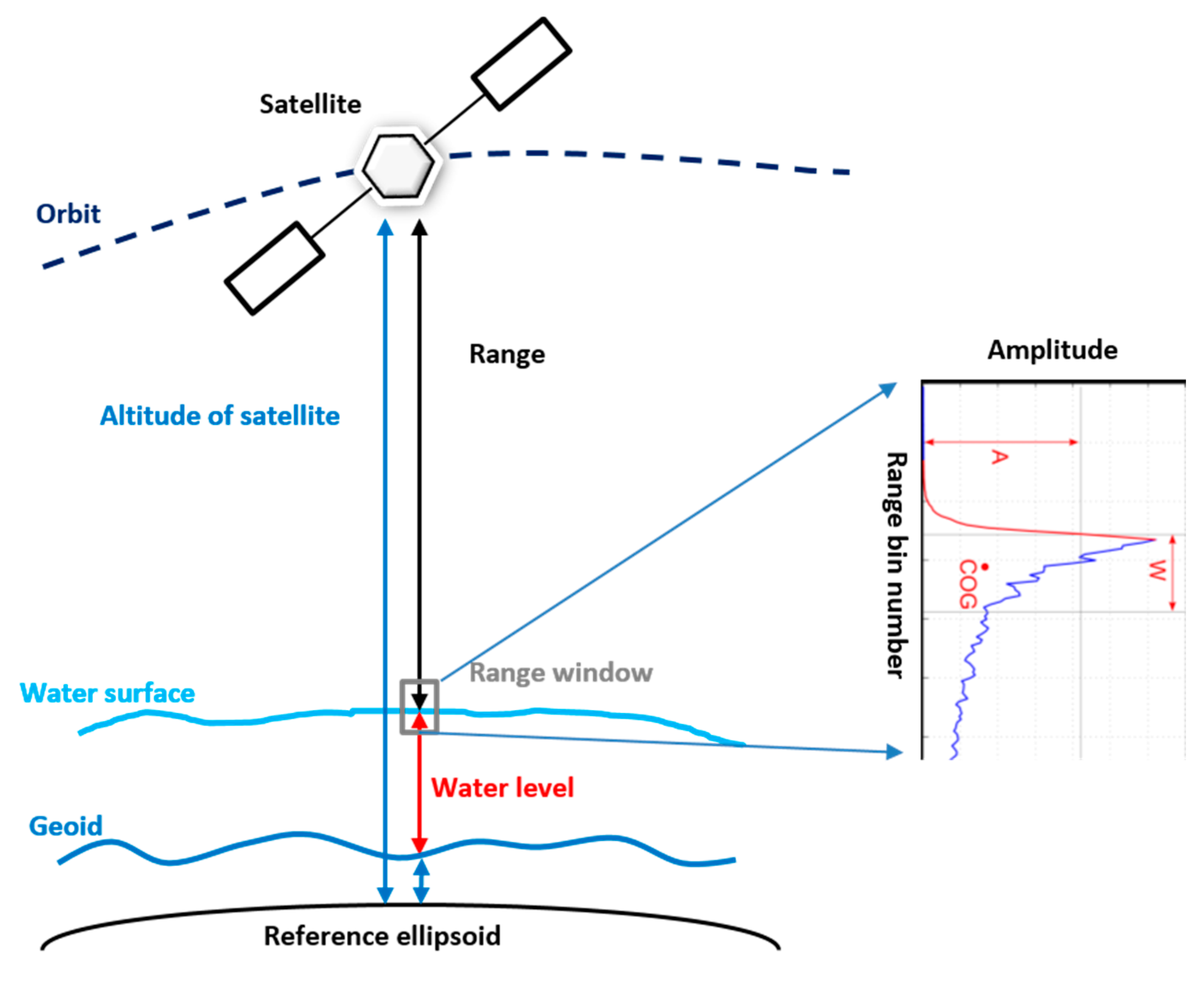
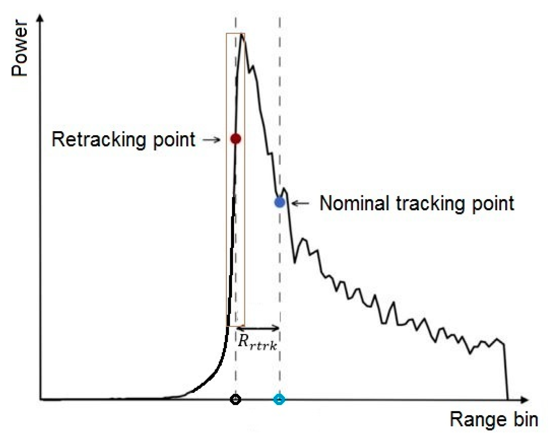
2. Basic Principles of Radar Altimetry
3. Mission Overview
3.1. Instrument
3.2. Orbit
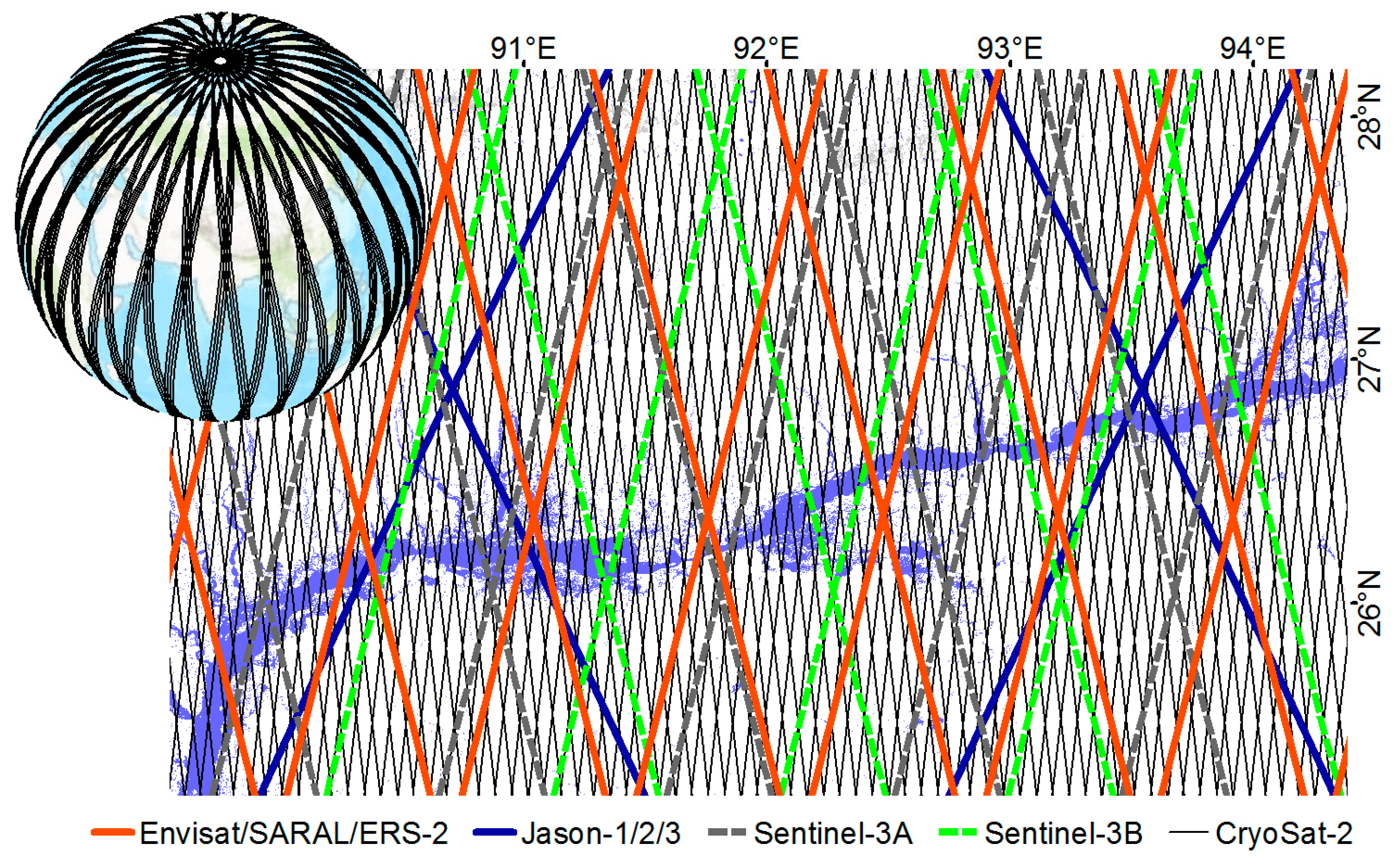
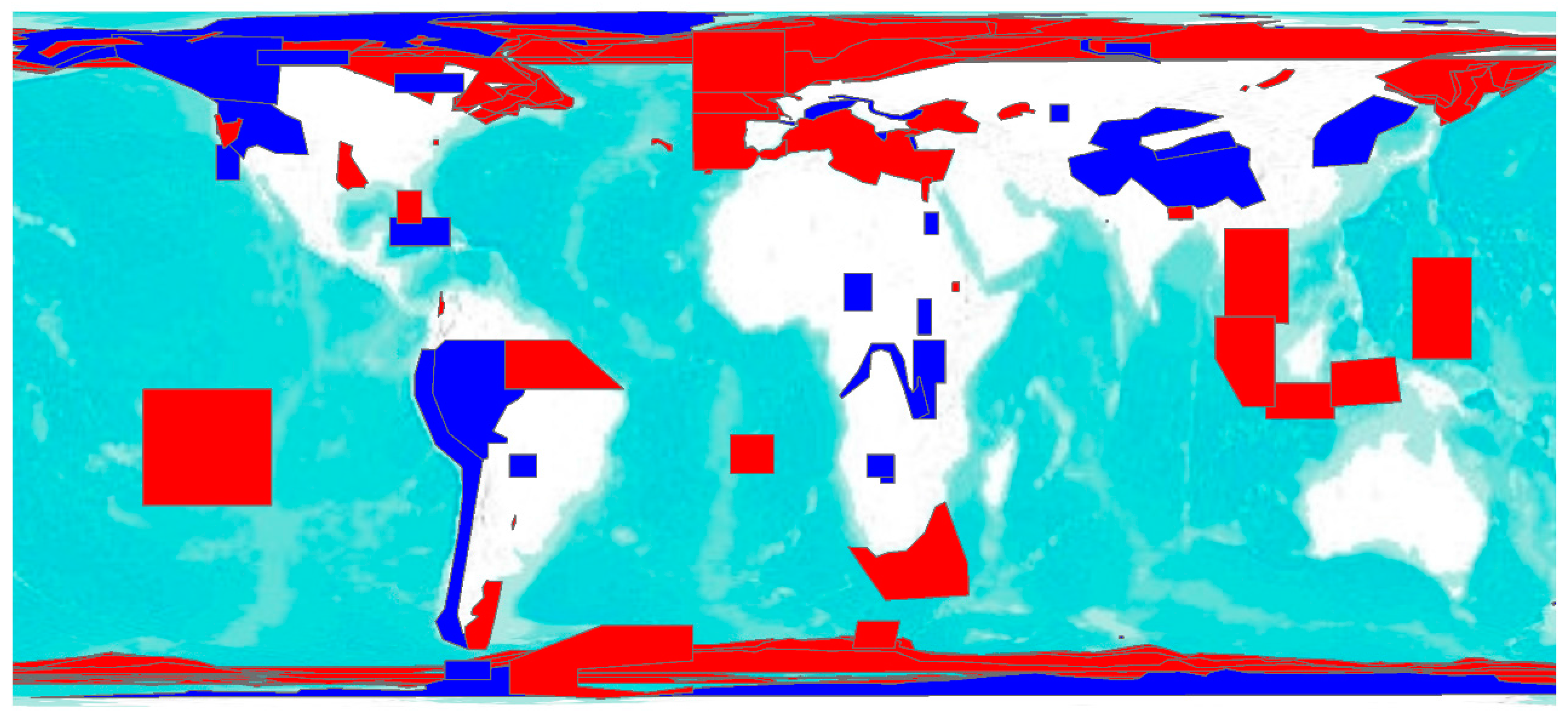
3.3. Ground Track
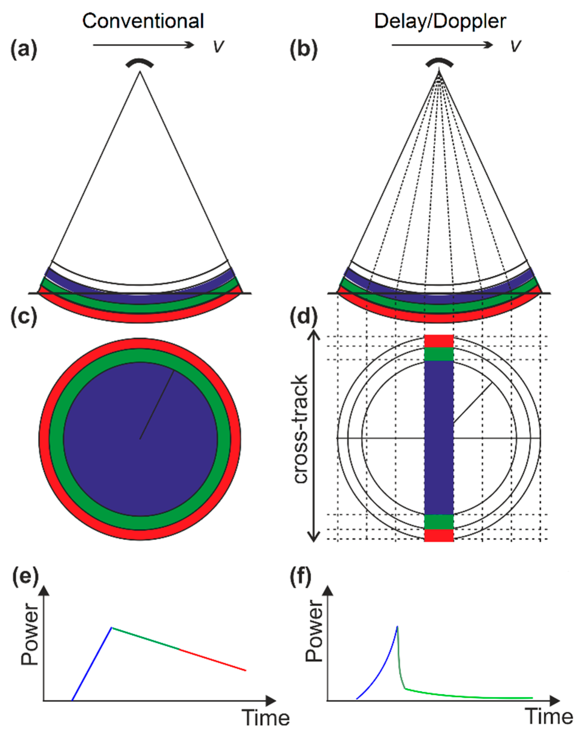
3.4. Footprint
4. Data Products
4.1. Level-1b Data
4.2. Level-2 GDR Data
4.3. Level-3 (Along-Track) Products
5. Use of CryoSat-2 over Lakes
5.1. Time Series Construction
5.2. Lake Level Trend Estimation
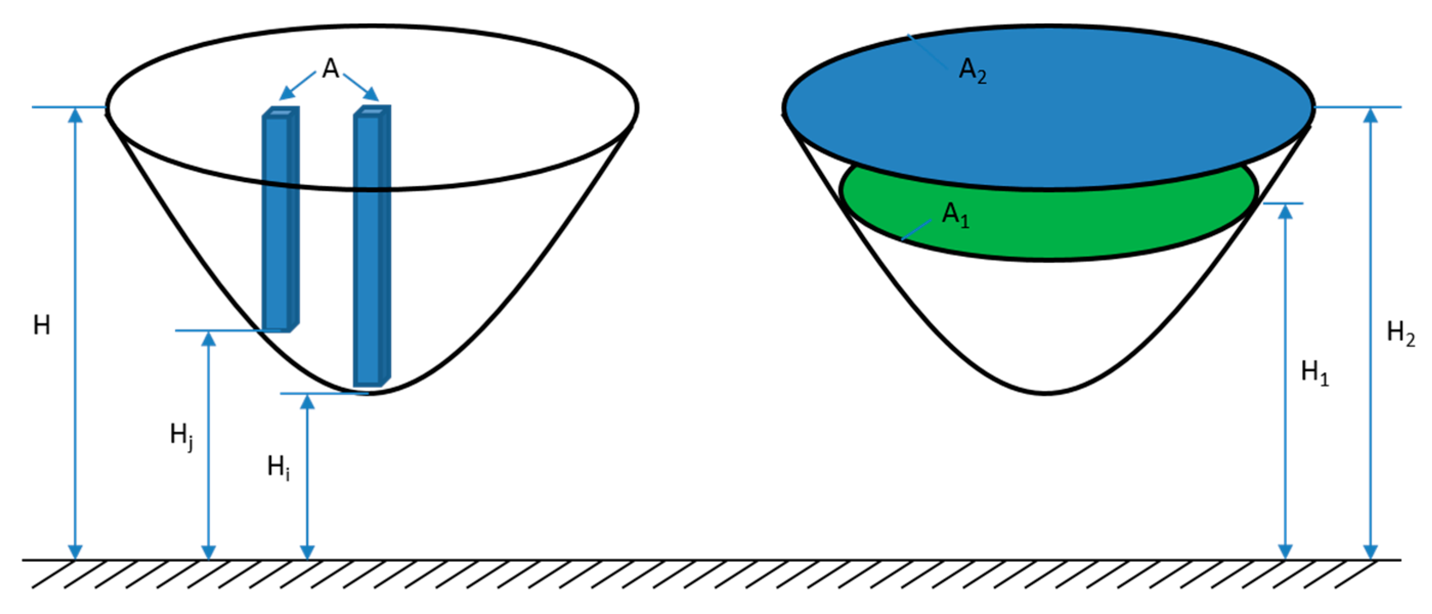
5.3. Lake Storage Calculation
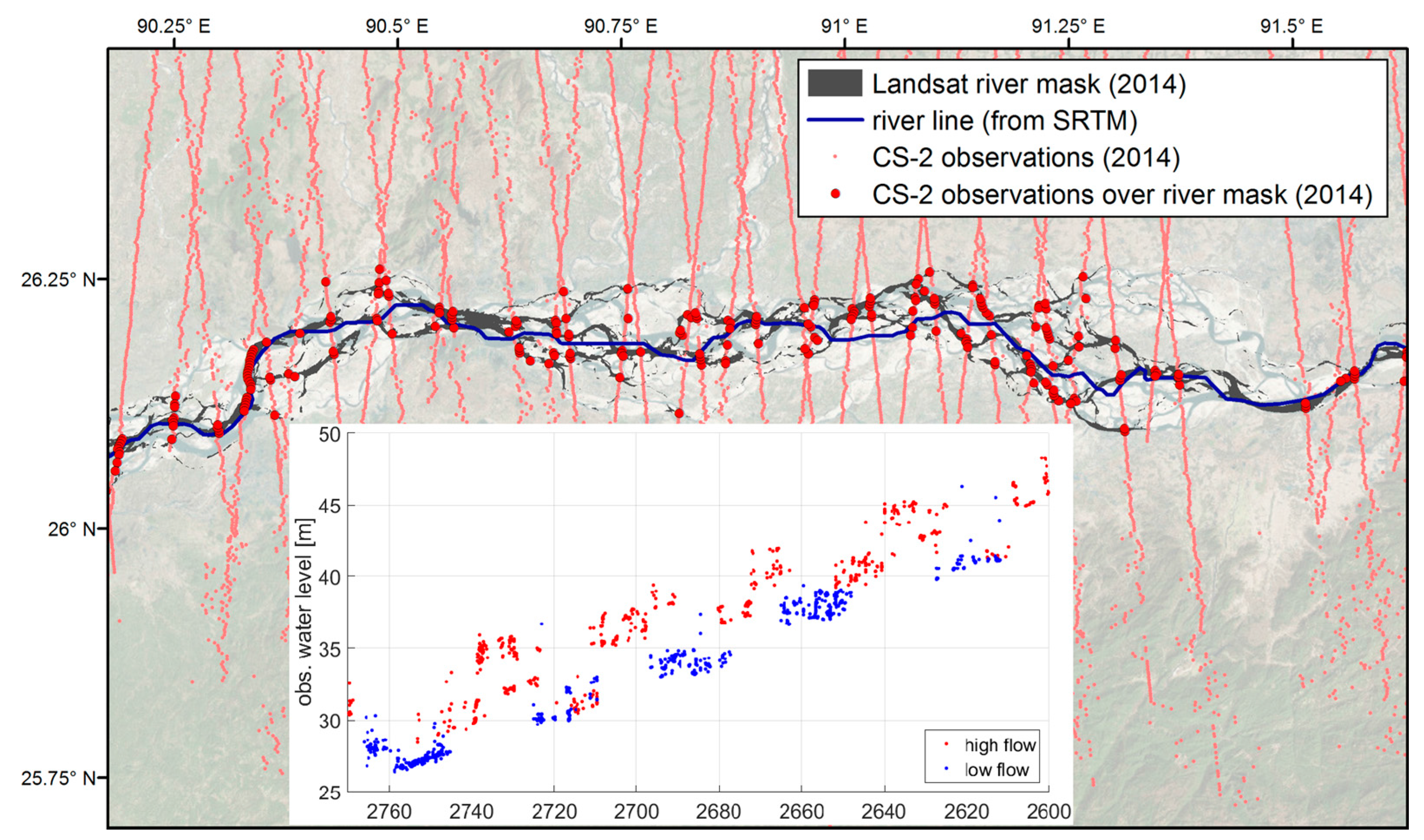
6. Use of CryoSat-2 over Rivers
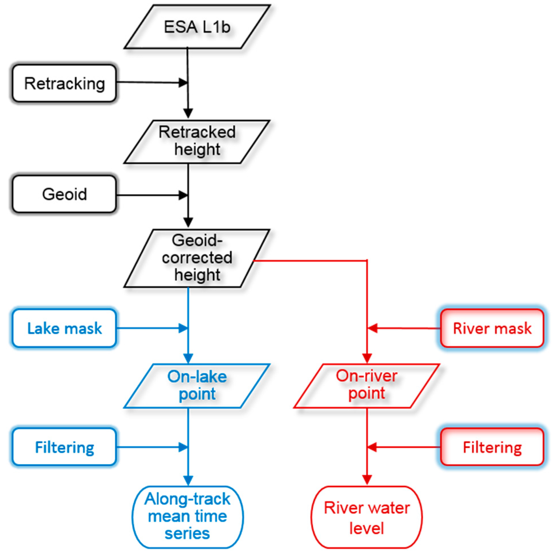
6.1. Masking and Filtering
6.2. Densification
6.3. Merging with Hydrodynamic Models
7. Discussion and Perspectives
8. Conclusions
Acknowledgments
Author Contributions
Conflicts of Interest
References
- Vorosmarty, C.J. Global Water Resources: Vulnerability from Climate Change and Population Growth. Science 2000, 289, 284–288. [Google Scholar] [CrossRef] [PubMed]
- Flood Fury: Why Brahmaputra’s Trail of Destruction Has Become Annual Ritual in Assam. The Indian Express. Available online: http://indianexpress.com/article/india/india-news-india/flood-fury-why-brahmapurtas-trail-of-destruction-has-become-annual-ritual-in-assam-2958587/ (accessed on 16 January 2017).
- United States Geological Survey (USGS). The Water Cycle. Available online: http://water.usgs.gov/edu/watercyclefreshstorage.html (accessed on 10 March 2017).
- Ma, R.; Duan, H.; Hu, C.; Feng, X.; Li, A.; Ju, W.; Jiang, J.; Yang, G. A half-century of changes in China’s lakes: Global warming or human influence? Geophys. Res. Lett. 2010, 37. [Google Scholar] [CrossRef]
- Oren, A.; Plotnikov, I.S.; Sokolov, S.S.; Aladin, N.V. The Aral Sea and the Dead Sea: Disparate lakes with similar histories. Lakes Reserv. Res. Manag. 2010, 15, 223–236. [Google Scholar] [CrossRef]
- Carroll, M.L.; Townshend, J.R.G.; Dimiceli, C.M.; Loboda, T.; Sohlberg, R.A. Shrinking lakes of the Arctic: Spatial relationships and trajectory of change. Geophys. Res. Lett. 2011, 38, 1–5. [Google Scholar] [CrossRef]
- Gao, H.; Bohn, T.J.; Podest, E.; McDonald, K.C.; Lettenmaier, D.P. On the causes of the shrinking of Lake Chad. Environ. Res. Lett. 2011, 6, 34021. [Google Scholar] [CrossRef]
- Tao, S.; Fang, J.; Zhao, X.; Zhao, S.; Shen, H.; Hu, H.; Tang, Z.; Wang, Z.; Guo, Q. Rapid loss of lakes on the Mongolian Plateau. Proc. Natl. Acad. Sci. USA 2015, 112, 2281–2286. [Google Scholar] [CrossRef] [PubMed]
- Pekel, J.-F.; Cottam, A.; Gorelick, N.; Belward, A.S. High-resolution mapping of global surface water and its long-term changes. Nature 2016, 540, 418–422. [Google Scholar] [CrossRef] [PubMed]
- Da Silva, J.S.; Calmant, S.; Seyler, F.; Moreira, D.M.; Oliveira, D.; Monteiro, A. Radar Altimetry Aids Managing Gauge Networks. Water Resour. Manag. 2014, 28, 587–603. [Google Scholar] [CrossRef]
- Global Runoff Data Center (GRDC). Global Runoff Database 2015. Available online: http://www.bafg.de/GRDC/EN/Home/homepage_node.html (accessed on 10 March 2017).
- Biancamaria, S.; Hossain, F.; Lettenmaier, D.P. Forecasting transboundary river water elevations from space. Geophys. Res. Lett. 2011, 38, 1–5. [Google Scholar] [CrossRef]
- Birkett, C.M. The contribution of TOPEX/POSEIDON to the global monitoring of climatically sensitive lakes. J. Geophys. Res. 1995, 100, 25179. [Google Scholar] [CrossRef]
- Berry, P.A.M.; Garlick, J.D.; Freeman, J.A.; Mathers, E.L. Global inland water monitoring from multi-mission altimetry. Geophys. Res. Lett. 2005, 32, 1–4. [Google Scholar] [CrossRef]
- Crétaux, J.F.; Birkett, C. Lake studies from satellite radar altimetry. C. R. Geosci. 2006, 338, 1098–1112. [Google Scholar] [CrossRef]
- Michailovsky, C.I.; Bauer-Gottwein, P. Operational reservoir inflow forecasting with radar altimetry: The Zambezi case study. Hydrol. Earth Syst. Sci. 2014, 18, 997–1007. [Google Scholar] [CrossRef]
- Kleinherenbrink, M.; Lindenbergh, R.C.; Ditmar, P.G. Monitoring of lake level changes on the Tibetan Plateau and Tian Shan by retracking Cryosat SARIn waveforms. J. Hydrol. 2015, 521, 119–131. [Google Scholar] [CrossRef]
- Nielsen, K.; Stenseng, L.; Andersen, O.B.; Villadsen, H.; Knudsen, P. Validation of CryoSat-2 SAR mode based lake levels. Remote Sens. Environ. 2015, 171, 162–170. [Google Scholar] [CrossRef]
- Villadsen, H.; Andersen, O.B.; Stenseng, L.; Nielsen, K.; Knudsen, P. CryoSat-2 altimetry for river level monitoring—Evaluation in the Ganges–Brahmaputra River basin. Remote Sens. Environ. 2015, 168, 80–89. [Google Scholar] [CrossRef]
- Zhang, G.; Yao, T.; Xie, H.; Kang, S.; Lei, Y. Increased mass over the Tibetan Plateau: From lakes or glaciers? Geophys. Res. Lett. 2013, 40, 2125–2130. [Google Scholar] [CrossRef]
- Jiang, L.; Nielsen, K.; Andersen, O.B.; Bauer-Gottwein, P. Monitoring recent lake level variations on the Tibetan Plateau using CryoSat-2 SARIn mode data. J. Hydrol. 2017, 544, 109–124. [Google Scholar] [CrossRef]
- Michailovsky, C.I.; Milzow, C.; Bauer-Gottwein, P. Assimilation of radar altimetry to a routing model of the Brahmaputra River. Water Resour. Res. 2013, 49, 4807–4816. [Google Scholar] [CrossRef]
- Maswood, M.; Hossain, F. Advancing River Modeling in Ungauged Basins using Satellite Remote Sensing: The case of the Ganges-Brahmaputra-Meghna basins. Int. J. River Basin Manag. 2016, 14, 103–117. [Google Scholar] [CrossRef]
- Paris, A.; de Paiva, R.D.; da Silva, J.S.; Moreira, D.M.; Calmant, S.; Garambois, P.-A.; Collischonn, W.; Bonnet, M.-P.; Seyler, F. Stage-discharge rating curves based on satellite altimetry andmodeled discharge in the Amazon basin. Water Resour. Res. 2016, 52, 3787–3814. [Google Scholar] [CrossRef]
- Semmling, M.; Beyerle, G.; Beckheinrich, J.; Ge, M.; Wickert, J. Airborne GNSS reflectometry using crossover reference points for carrier phase altimetry. In Proceedings of the 2014 IEEE International Geoscience and Remote Sensing Symposium, Quebec City, QC, Canada, 13–18 July 2014; pp. 3786–3789.
- Jin, S.; Komjathy, A. GNSS reflectometry and remote sensing: New objectives and results. Adv. Space Res. 2010, 46, 111–117. [Google Scholar] [CrossRef]
- Richter, A.; Popov, S.V.; Fritsche, M.; Lukin, V.V.; Matveev, A.Y.; Ekaykin, A.A.; Lipenkov, V.Y.; Fedorov, D.V.; Eberlein, L.; Schröder, L.; et al. Height changes over subglacial Lake Vostok, East Antarctica: Insights from GNSS observations. J. Geophys. Res. Earth Surf. 2014, 119, 2460–2480. [Google Scholar] [CrossRef]
- Asadzadeh Jarihani, A.; Callow, J.N.; Johansen, K.; Gouweleeuw, B. Evaluation of multiple satellite altimetry data for studying inland water bodies and river floods. J. Hydrol. 2013, 505, 78–90. [Google Scholar] [CrossRef]
- Ricker, R.; Hendricks, S.; Helm, V.; Gerdes, R. Classification of CryoSat-2 radar echoes. In Towards an Interdisciplinary Approach in Earth System Science: Advances of a Helmholtz Graduate Research School; Springer: Cham, Switzerland, 2015; pp. 149–158. [Google Scholar]
- Schneider, R.; Godiksen, P.N.; Villadsen, H.; Madsen, H.; Bauer-Gottwein, P. Application of CryoSat-2 altimetry data for river analysis and modelling. Hydrol. Earth Syst. Sci. 2017, 21, 751–764. [Google Scholar] [CrossRef]
- Göttl, F.; Dettmering, D.; Müller, F.; Schwatke, C. Lake Level Estimation Based on CryoSat-2 SAR Altimetry and Multi-Looked Waveform Classification. Remote Sens. 2016, 8, 885. [Google Scholar] [CrossRef]
- Villadsen, H.; Deng, X.; Andersen, O.B.; Stenseng, L.; Nielsen, K.; Knudsen, P. Improved inland water levels from SAR altimetry using novel empirical and physical retrackers. J. Hydrol. 2016, 537, 234–247. [Google Scholar] [CrossRef]
- Chelton, D.B.; Ries, J.C.; Haines, B.J.; Fu, L.-L.; Callahan, P.S. Satellite altimetry. In Satellite Altimetry and Earth Sciences: A Handbook of Techniques and Applications; Academic Press: Cambridge, MA, USA, 2001; Volume 69, pp. 2504–2510. [Google Scholar]
- European Space Agency. Mullar Space Science Laboratory CryoSat Product Handbook; European Space Agency: Paris, France, 2012; Volume DLFE-3605, Available online: https://earth.esa.int/c/document_library/get_file?folderId=125272&name=DLFE-3605.pdf (accessed on 27 January 2017).
- Jain, M.; Andersen, O.B.; Dall, J. Improved Sea Level Determination in the Arctic Regions through Development of Tolerant Altimetry Retracking; Technical University of Denmark: Kgs. Lyngby, Denmark, 2015. [Google Scholar]
- Rosmorduc, V.; Benveniste, J.; Lauret, O.; Maheu, C.; Milagro, M.; Picot, N. Radar Altimetry Tutorial; Benveniste, J., Picot, N., Eds.; European Space Agency: Paris, France, 2011. [Google Scholar]
- Bao, L.; Lu, Y.; Wang, Y. Improved retracking algorithm for oceanic altimeter waveforms. Prog. Nat. Sci. 2009, 19, 195–203. [Google Scholar] [CrossRef]
- Jain, M.; Andersen, O.B.; Dall, J.; Stenseng, L. Sea surface height determination in the Arctic using Cryosat-2 SAR data from primary peak empirical retrackers. Adv. Space Res. 2015, 55, 40–50. [Google Scholar] [CrossRef]
- Davis, C.H. Growth of the Greenland ice sheet: A performance assessment of altimeter retracking algorithms. IEEE Trans. Geosci. Remote Sens. 1995, 33, 1108–1116. [Google Scholar] [CrossRef]
- European Space Agency. CryoSat Level-2 Product Evolutions and Quality Improvements in Baseline C. 2015. Available online: https://earth.esa.int/documents/10174/1773005/C2-Evolution-BaselineC-Level2-V3 (accessed on 27 January 2017).
- Birkett, C.M.; Beckley, B.D. Investigating the Performance of the Jason-2/OSTM Radar Altimeter over Lakes and Reservoirs. Mar. Geod. 2010, 33, 204–238. [Google Scholar] [CrossRef]
- Geographical Mode Mask. Content—Earth Online—ESA. Available online: https://earth.esa.int/web/guest/-/geographical-mode-mask-7107 (accessed on 16 January 2017).
- Wingham, D.J.; Francis, C.R.; Baker, S.; Bouzinac, C.; Brockley, D.; Cullen, R.; de Chateau-Thierry, P.; Laxon, S.W.; Mallow, U.; Mavrocordatos, C.; et al. CryoSat: A mission to determine the fluctuations in Earth’s land and marine ice fields. Adv. Space Res. 2006, 37, 841–871. [Google Scholar] [CrossRef]
- Ulaby, F.T.; Long, D.G.; Blackwell, W.J.; Elachi, C.; Fung, A.K.; Ruf, C.; Sarabandi, K.; Zebker, H.A.; van Zyl, J. Microwave Radar and Radiometric Remote Sensing; University of Michigan Press: Ann Arbor, MI, USA, 2014. [Google Scholar]
- Soussi, B. ENVISAT ALTIMETRY Level 2 User Manual. Available online: https://earth.esa.int/pub/ESA_DOC/ENVISAT/RA2-MWR/PH_light_1rev4_ESA.pdf (accessed on 27 January 2017).
- Fetterer, F.M.; Drinkwater, M.R.; Jezek, K.C.; Laxon, S.W.C.; Onstott, R.G.; Ulander, L.M.H. Sea ice altimetry. In Microwave Remote Sensing of Sea Ice; Carsey, F.D., Ed.; Geophysical Monograph Series; American Geophysical Union (AGU): Washington, DC, USA, 1992; Volume 68, pp. 111–135. [Google Scholar]
- Keith Raney, R. The delay/doppler radar altimeter. IEEE Trans. Geosci. Remote Sens. 1998, 36, 1578–1588. [Google Scholar] [CrossRef]
- Kleinherenbrink, M.; Ditmar, P.G.; Lindenbergh, R.C. Retracking Cryosat data in the SARIn mode and robust lake level extraction. Remote Sens. Environ. 2014, 152, 38–50. [Google Scholar] [CrossRef]
- Schwatke, C.; Dettmering, D.; Bosch, W.; Seitz, F. DAHITI—An innovative approach for estimating water level time series over inland waters using multi-mission satellite altimetry. Hydrol. Earth Syst. Sci. 2015, 19, 4345–4364. [Google Scholar] [CrossRef]
- Tourian, M.J.; Tarpanelli, A.; Elmi, O.; Qin, T.; Brocca, L.; Moramarco, T.; Sneeuw, N. Spatiotemporal densification of river water level time series by multimission satellite altimetry. Water Resour. Res. 2016, 52, 1140–1159. [Google Scholar] [CrossRef]
- Song, C.; Ye, Q.; Cheng, X. Shifts in water-level variation of Namco in the central Tibetan Plateau from ICESat and CryoSat-2 altimetry and station observations. Sci. Bull. 2015, 60, 1287–1297. [Google Scholar] [CrossRef]
- Tourian, M.J.; Elmi, O.; Chen, Q.; Devaraju, B.; Roohi, S.; Sneeuw, N. A spaceborne multisensor approach to monitor the desiccation of Lake Urmia in Iran. Remote Sens. Environ. 2015, 156, 349–360. [Google Scholar] [CrossRef]
- Zhang, G.; Xie, H.; Kang, S.; Yi, D.; Ackley, S.F. Monitoring lake level changes on the Tibetan Plateau using ICESat altimetry data (2003–2009). Remote Sens. Environ. 2011, 115, 1733–1742. [Google Scholar] [CrossRef]
- Gao, L.; Liao, J.; Shen, G. Monitoring lake-level changes in the Qinghai–Tibetan Plateau using radar altimeter data (2002–2012). J. Appl. Remote Sens. 2013, 7, 73470. [Google Scholar] [CrossRef]
- Li, Y.; Liao, J.; Guo, H.; Liu, Z.; Shen, G. Patterns and potential drivers of dramatic changes in Tibetan lakes, 1972–2010. PLoS ONE 2014, 9, e111890. [Google Scholar] [CrossRef] [PubMed]
- Song, C.; Huang, B.; Ke, L. Heterogeneous change patterns of water level for inland lakes in High Mountain Asia derived from multi-mission satellite altimetry. Hydrol. Process. 2015, 29, 2769–2781. [Google Scholar] [CrossRef]
- Taube, C.M. Chapter 12: Three methods for computing the volume of a lake. In Manual of Fisheries Survey Mehtods II: With Periodic Updates; Schneider, J.C., Ed.; Michigan Department of Natural Resources: Lansing, MI, USA, 2000. [Google Scholar]
- Phan, V.H.; Lindenbergh, R.; Menenti, M. ICESat derived elevation changes of Tibetan lakes between 2003 and 2009. Int. J. Appl. Earth Obs. Geoinf. 2012, 17, 12–22. [Google Scholar] [CrossRef]
- Baup, F.; Frappart, F.; Maubant, J. Combining high-resolution satellite images and altimetry to estimate the volume of small lakes. Hydrol. Earth Syst. Sci. 2014, 18, 2007–2020. [Google Scholar] [CrossRef]
- Dehecq, A.; Gourmelen, N.; Shepherd, A.; Cullen, R.; Trouvé, E. Evaluation of CryoSat-2 for height retrieval over the Himalayan range. In Proceedings of the CryoSat-2 Third User Workshop, Dresden, Germany, 12–14 March 2013.
- Rosmorduc, V. Hydroweb Product User Manual Version 1.0; Theia—Land Data Centre: Ramonville-Saint-Agne, France, 2016. [Google Scholar]
- Berry, P.A.M.; Wheeler, J.L. JASON2-ENVISAT Exploitation—Development of Algorithms for the Exploitation of JASON2-ENVISAT Altimetry for the Generation of a River and Lake Product; Product Handbook v3.5; De Montfort University: Leicester, UK, 2009. [Google Scholar]
- Michailovsky, C.I.; McEnnis, S.; Berry, P.A.M.; Smith, R.; Bauer-Gottwein, P. River monitoring from satellite radar altimetry in the Zambezi River basin. Hydrol. Earth Syst. Sci. 2012, 16, 2181–2192. [Google Scholar] [CrossRef]
- Paiva, R.C.D.; Durand, M.T.; Hossain, F. Spatiotemporal interpolation of discharge across a river network by using synthetic SWOT satellite data. Water Resour. Res. 2015, 51, 430–449. [Google Scholar] [CrossRef]
- Yoon, Y.; Durand, M.; Merry, C.J.; Rodriguez, E. Improving temporal coverage of the SWOT mission using spatiotemporal kriging. IEEE J. Sel. Top. Appl. Earth Obs. Remote Sens. 2013, 6, 1719–1729. [Google Scholar] [CrossRef]
- Boergens, E.; Buhl, S.; Dettmering, D.; Klüppelberg, C.; Seitz, F. Combination of multi-mission altimetry data along the Mekong River with spatio-temporal kriging. J. Geod. 2016. [Google Scholar] [CrossRef]
- Bercher, N.; Dinardo, S.; Lucas, B.M.; Fleury, S.; Calmant, S.; Crétaux, J.-F.; Femenias, P.; Boy, F.; Picot, N.; Benveniste, J. Applications of CryoSat-2 SAR & SARIn modes for the monitoring of river water levels. In Proceedings of the CryoSat Third User Workshop, Dresden, Germany, 12–14 March 2013; pp. 1–7.
- Lettenmaier, D.P.; Alsdorf, D.; Dozier, J.; Huffman, G.J.; Pan, M.; Wood, E.F. Inroads of remote sensing into hydrologic science during the WRR era. Water Resour. Res. 2015, 51, 7309–7342. [Google Scholar] [CrossRef]
- Domeneghetti, A.; Tarpanelli, A.; Brocca, L.; Barbetta, S.; Moramarco, T.; Castellarin, A.; Brath, A. The use of remote sensing-derived water surface data for hydraulic model calibration. Remote Sens. Environ. 2014, 149, 130–141. [Google Scholar] [CrossRef]
- Yan, K.; Tarpanelli, A.; Balint, G.; Moramarco, T.; Di Baldassarre, G. Exploring the Potential of SRTM Topography and Radar Altimetry to Support Flood Propagation Modeling: Danube Case Study. J. Hydrol. Eng. 2014, 20, 04014048. [Google Scholar] [CrossRef]
- Biancamaria, S.; Bates, P.D.; Boone, A.; Mognard, N.M. Large-scale coupled hydrologic and hydraulic modelling of the Ob River in Siberia. J. Hydrol. 2009, 379, 136–150. [Google Scholar] [CrossRef]
- Paiva, R.C.D.; Collischonn, W.; Bonnet, M.-P.; de Gonçalves, L.G.G.; Calmant, S.; Getirana, A.; da Santos Silva, J. Assimilating in situ and radar altimetry data into a large-scale hydrologic-hydrodynamic model for streamflow forecast in the Amazon. Hydrol Earth Syst. Sci. 2013, 10, 2879–2925. [Google Scholar]
- Hossain, F.; Maswood, M.; Siddique-E-Akbor, A.H.; Yigzaw, W.; Mazumdar, L.C.; Ahmed, T.; Hossain, M.; Shah-Newaz, S.M.; Limaye, A.; Lee, H.; et al. A promising radar altimetry satellite system for operational flood forecasting in flood-prone Bangladesh. IEEE Geosci. Remote Sens. Mag. 2014, 2, 27–36. [Google Scholar] [CrossRef]
- Schneider, R.; Godiksen, P.N.; Ridler, M.-E.; Villadsen, H.; Madsen, H.; Bauer-Gottwein, P. Combining Envisat type and CryoSat-2 altimetry to inform hydrodynamic models. In Proceedings Living Planet Symposium 2016; Ouwehand, L., Ed.; ESA Special Publications SP-740; European Space Agency: Paris, France, 2016. [Google Scholar]
- O’Loughlin, F.; Trigg, M.A.; Schumann, G.J.P.; Bates, P.D. Hydraulic characterization of the middle reach of the Congo River. Water Resour. Res. 2013, 49, 5059–5070. [Google Scholar] [CrossRef]
- Cotton, P.D.; Andersen, O.; Stenseng, L.; Boy, F.; Cancet, M.; Cipollini, P.; Gommenginger, C.; Dinardo, S.; Egido, A.; Fernandes, M.J.; et al. Improved Oceanographic Measurements from SAR Altimetry: Results and Scientific Roadmap from ESA Cryosat Plus for Oceans Project; Special Publication ESA SP 2016; European Space Agency: Paris, France, 2016. [Google Scholar]
- Maillard, P.; Bercher, N.; Calmant, S. New processing approaches on the retrieval of water levels in Envisat and SARAL radar altimetry over rivers: A case study of the São Francisco River, Brazil. Remote Sens. Environ. 2015, 156, 226–241. [Google Scholar] [CrossRef]
- Yamazaki, D.; O’Loughlin, F.; Trigg, M.A.; Miller, Z.F.; Pavelsky, T.M.; Bates, P.D. Development of the Global Width Database for Large Rivers. Water Resour. Res. 2014, 50, 3467–3480. [Google Scholar] [CrossRef]
- Andreadis, K.M.; Schumann, G.J.P.; Pavelsky, T. A simple global river bankfull width and depth database. Water Resour. Res. 2013, 49, 7164–7168. [Google Scholar] [CrossRef]
- Biancamaria, S.; Lettenmaier, D.P.; Pavelsky, T.M. The SWOT Mission and Its Capabilities for Land Hydrology. Surv. Geophys. 2016, 37, 307–337. [Google Scholar] [CrossRef]
- Biancamaria, S.; Durand, M.; Andreadis, K.M.; Bates, P.D.; Boone, A.; Mognard, N.M.; Rodríguez, E.; Alsdorf, D.E.; Lettenmaier, D.P.; Clark, E.A. Assimilation of virtual wide swath altimetry to improve Arctic river modeling. Remote Sens. Environ. 2011, 115, 373–381. [Google Scholar] [CrossRef]
- Yoon, Y.; Durand, M.; Merry, C.J.; Clark, E.A.; Andreadis, K.M.; Alsdorf, D.E. Estimating river bathymetry from data assimilation of synthetic SWOT measurements. J. Hydrol. 2012, 464–465, 363–375. [Google Scholar] [CrossRef]
- Durand, M.; Neal, J.; Rodríguez, E.; Andreadis, K.M.; Smith, L.C.; Yoon, Y. Estimating reach-averaged discharge for the River Severn from measurements of river water surface elevation and slope. J. Hydrol. 2014, 511, 92–104. [Google Scholar] [CrossRef]
- Garambois, P.-A.; Monnier, J. Inference of effective river properties from remotely sensed observations of water surface. Adv. Water Resour. 2015, 79, 103–120. [Google Scholar] [CrossRef]


| Satellite | Agency | Period | Altitude (km) | Altimeter | Frequency Used | Repetitivity (Day) | Equatorial Inter-Track Distance (km) |
|---|---|---|---|---|---|---|---|
| Skylab | NASA | May 1973–February 1974 | 435 | S193 | Ku-band | ||
| GEOS 3 | NASA | April 1975–July 1979 | 845 | ALT | Ku and C-band | ||
| SeaSat | NASA | July–October 1978 | 800 | ALT | Ku-band | 17 | |
| Geosat | US Navy | October 1985–January 1990 | 800 | Ku-band | 17 | ||
| ERS-1 | ESA | July 1991–March 2000 | 785 | RA | Ku-band | 35 | 80 |
| Topex/Poseidon | NASA/CNES | September 1992–October 2005 | 1336 | Poseidon | Ku and C-band | 10 | 315 |
| ERS-2 | ESA | April 1995–July 2011 | 785 | RA | Ku-band | 35 | 80 |
| GFO | US Navy/NOAA | February 1998–October 2008 | 800 | GFO-RA | Ku-band | 17 | 165 |
| Jason-1 | CNES/NASA | December 2001–June 2013 | 1336 | Poseidon-2 | Ku and C-band | 10 | 315 |
| Envisat | ESA | March 2002–April 2012 | 800 | RA-2 | Ku and S-band | 35 | 80 |
| OSTM/Jason-2 | CNES/NASA/Eumetsat/NOAA | Jun 2008–present | 1336 | Poseidon-3 | Ku and C-band | 10 | 315 |
| CryoSat-2 | ESA | April 2010–present | 720 | SIRAL | Ku-band | 369 | 7.5 |
| HY-2 | China | August 2011–present | 971 | Ku and C-band | 14, 168 | ||
| Saral | ISRO/CNES | February 2013–present | 800 | AltiKa | Ka-band | 35 | 80 |
| Jason-3 | CNES/NASA/Eumetsat/NOAA | January 2016–present | 1336 | Poseidon-3B | Ku and C-band | 10 | 315 |
| Sentinel-3A | ESA | February 2016–present | 814 | SRAL | Ku and C-band | 27 | 104 |
© 2017 by the authors. Licensee MDPI, Basel, Switzerland. This article is an open access article distributed under the terms and conditions of the Creative Commons Attribution (CC BY) license ( http://creativecommons.org/licenses/by/4.0/).
Share and Cite
Jiang, L.; Schneider, R.; Andersen, O.B.; Bauer-Gottwein, P. CryoSat-2 Altimetry Applications over Rivers and Lakes. Water 2017, 9, 211. https://doi.org/10.3390/w9030211
Jiang L, Schneider R, Andersen OB, Bauer-Gottwein P. CryoSat-2 Altimetry Applications over Rivers and Lakes. Water. 2017; 9(3):211. https://doi.org/10.3390/w9030211
Chicago/Turabian StyleJiang, Liguang, Raphael Schneider, Ole B. Andersen, and Peter Bauer-Gottwein. 2017. "CryoSat-2 Altimetry Applications over Rivers and Lakes" Water 9, no. 3: 211. https://doi.org/10.3390/w9030211
APA StyleJiang, L., Schneider, R., Andersen, O. B., & Bauer-Gottwein, P. (2017). CryoSat-2 Altimetry Applications over Rivers and Lakes. Water, 9(3), 211. https://doi.org/10.3390/w9030211