To What Extent Are Swiss Springs Refugial Habitats for Sensitive and Endangered Diatom Taxa?


Abstract
:1. Introduction
2. Materials and Methods
2.1. Sampling and Laboratory Methods
2.2. Identification
2.3. Species Lists
2.4. Species Red List Status and Rareness Weighting
2.5. Spring Alteration Degree (SAD)
2.6. Statistical Analyses
3. Results
3.1. Species Richness
3.2. Red List Status
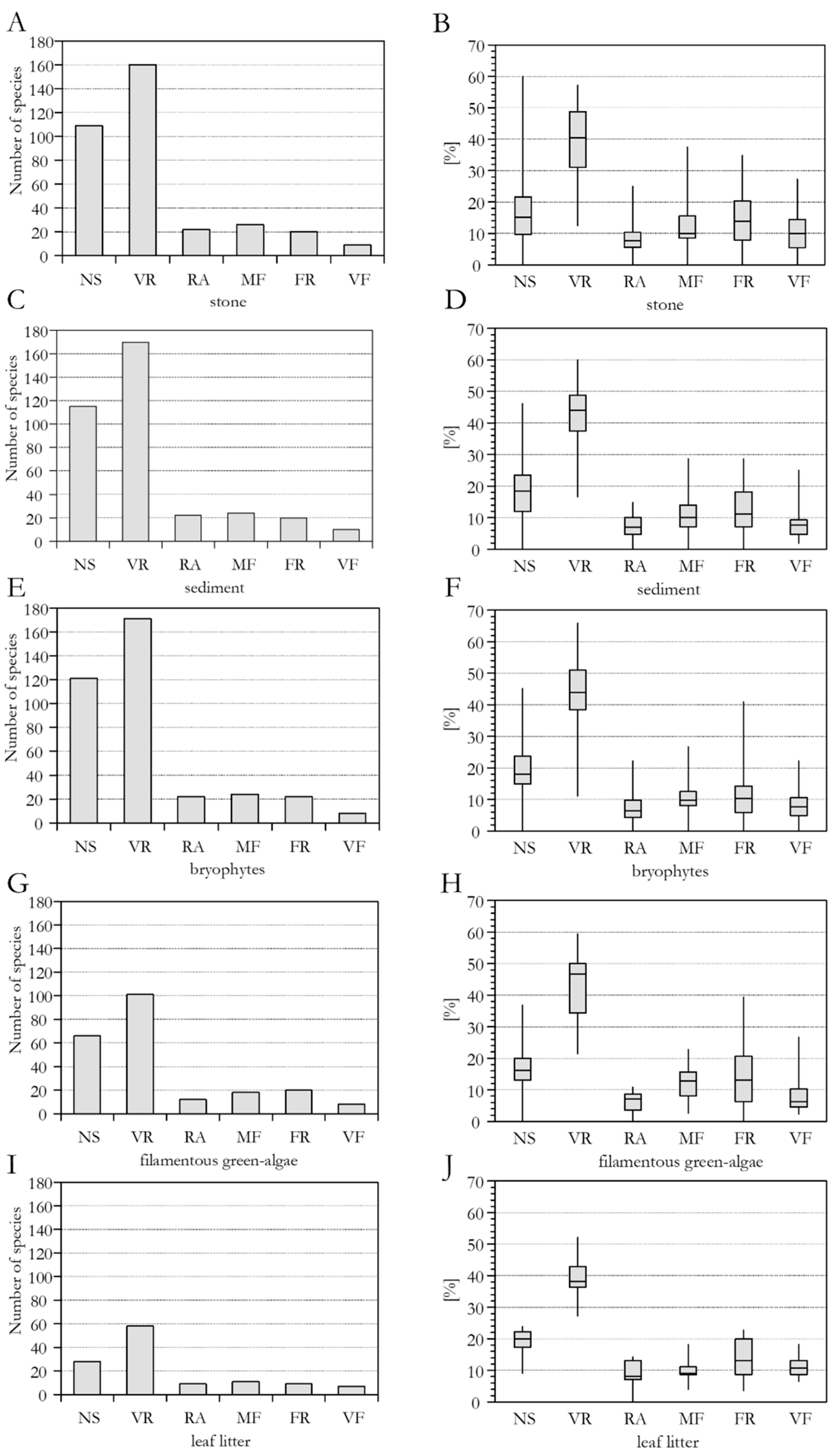
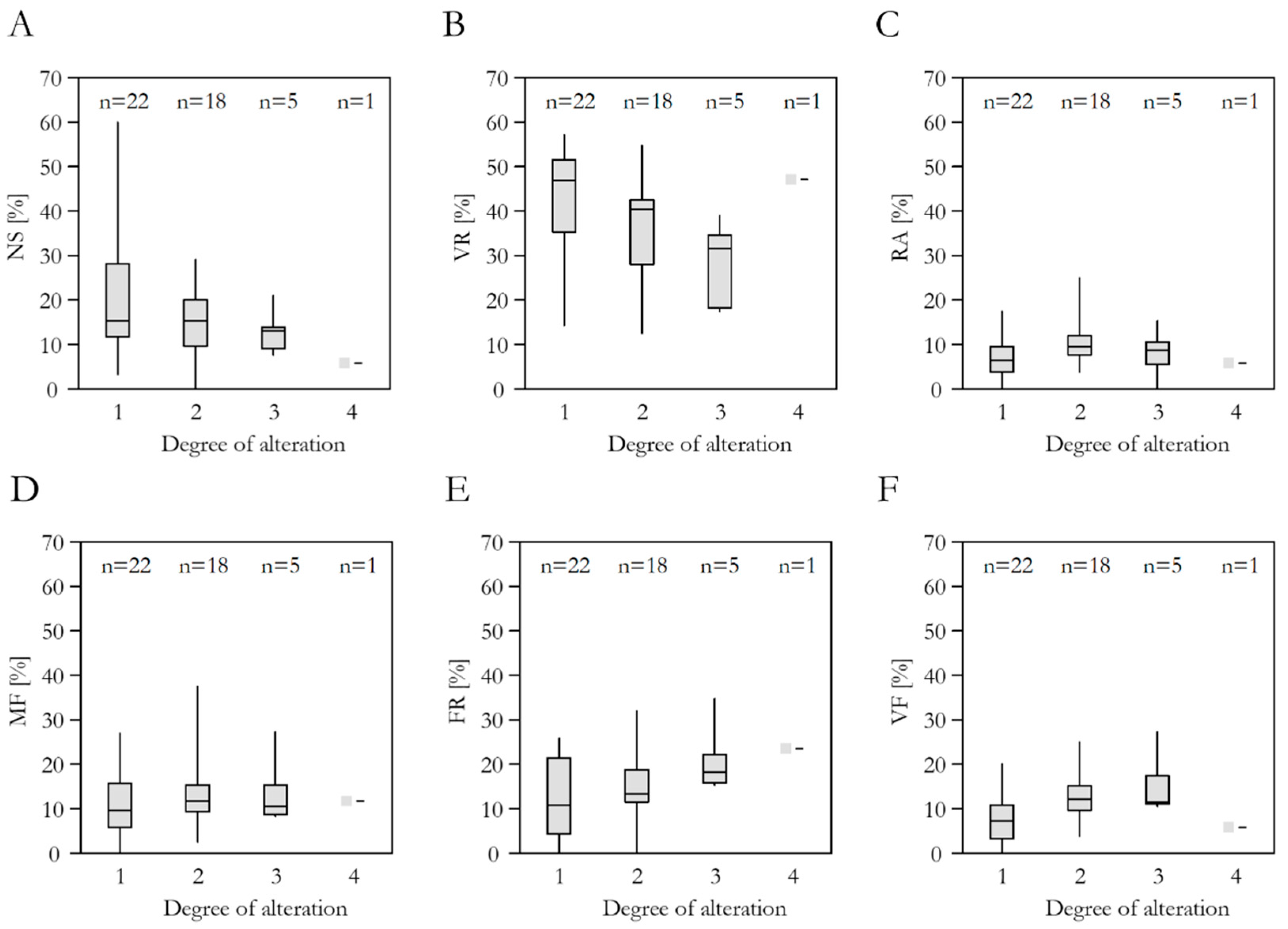
3.3. Species Frequency
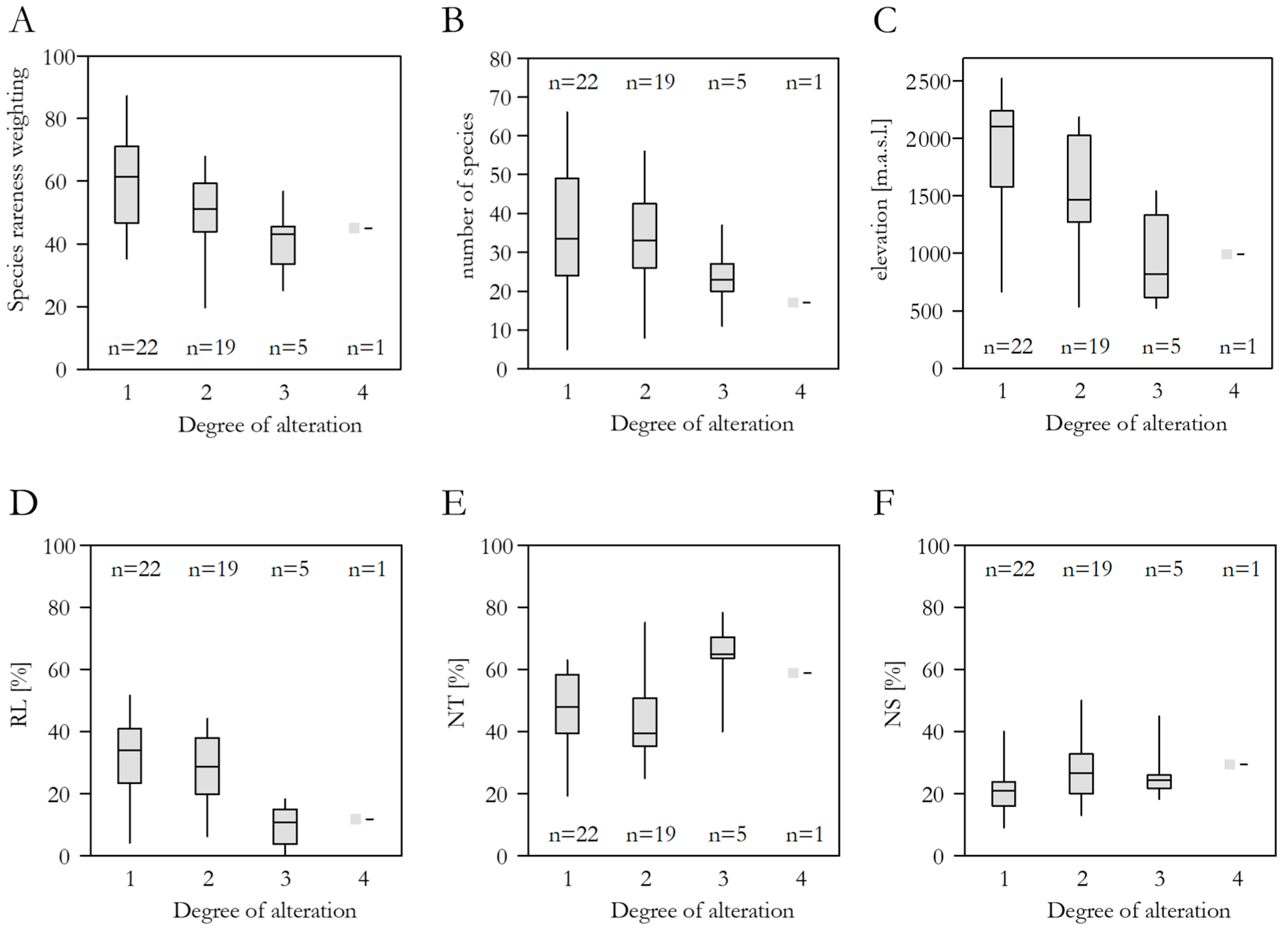
3.4. Spring Alteration Degree (SAD)
3.5. Species Richness, Red List Threat Status, Frequency in the DI-CH, and Spring Alteration Degree (SAD)
4. Discussion
Supplementary Materials
Supplementary File 1Acknowledgments
Author Contributions
Conflicts of Interest
References
- Strayer, D.L.; Dudgeon, D. Freshwater biodiversity conservation: Recent progress and future challenges. J. N. Am. Benthol. Soc. 2010, 29, 344–358. [Google Scholar]
- Baur, B.; Duelli, P.; Edwards, P.J.; Jenny, M.; Klaus, G.; Künzle, I.; Martinez, S.; Pauli, D.; Peter, K.; Schmid, B.; et al. Biodiversität der Schweiz: Zustand, Erhaltung, Perspektive. Wissenschaftliche Grundlagen für eine Nationale Strategie; Haupt Verlag: Bern, Germany, 2004; p. 236. [Google Scholar]
- Dudgeon, D.; Arthington, A.H.; Gessner, M.O.; Kawabata, Z.I.; Knowler, D.J.; Leveque, C.; Naiman, R.J.; Prieur-Richard, A.H.; Soto, D.; Stiassny, M.L.J.; et al. Freshwater biodiversity: Importance, threats, status and conservation challenges. Biol. Rev. 2006, 81, 163–182. [Google Scholar] [PubMed]
- Cantonati, M.; Füreder, L.; Gerecke, R.; Jüttner, I.; Cox, E.J. Crenic habitats, hotspots for freshwater biodiversity conservation: Toward an understanding of their ecology. Freshw. Sci. 2012, 31, 463–480. [Google Scholar] [CrossRef]
- Gerecke, R.; Franz, H.; Cantonati, M. Invertebrate diversity in springs of the National Park Berchtesgaden (Germany): Relevance for long-term monitoring. Verh. Internat. Verein. Limnol. 2009, 30, 1229–1233. [Google Scholar]
- Zechmeister, H.; Mucina, L. Vegetation of European springs—High-rank syntaxa of the Montio-Mardaminetea. J. Veg. Sci. 1994, 5, 385–402. [Google Scholar] [CrossRef]
- Werum, M.; Lange-Bertalot, H. Diatoms in Springs from Central Europe and Elsewhere under the Influence of Hydrogeology and Anthropogenic Impacts; A.R.G. Gantner Verlag K.G.: Ruggell, Liechtenstein, 2004; p. 480. [Google Scholar]
- Van der Kamp, G. The hydrogeology of springs in relation to the biodiversity of spring fauna—A review. J. Kans. Entomol. Soc. 1995, 68, 4–17. [Google Scholar]
- Cantonati, M.; Gerecke, R.; Bertuzzi, E. Springs of the Alps—Sensitive ecosystems to environmental change: From biodiversity assessments to long-term studies. Hydrobiologia 2006, 562, 59–96. [Google Scholar]
- Fránkóva, M.; Bojkova, J.; Poulickova, A.; Hajek, M. The structure and species richness of the diatom assemblages of the western Carpathian spring fens along the gradient of mineral richness. Fottea 2009, 9, 355–368. [Google Scholar] [CrossRef]
- Gesierich, D.; Kofler, W. Epilithic diatoms form rheocrene springs in the eastern Alps (Vorarlberg, Austria). Diatom Res. 2010, 25, 43–66. [Google Scholar] [CrossRef]
- Żelazna-Wieczorek, J. Diatom Flora in Springs of Lódz Hills (Central Poland). Biodiversity, Taxonomy, and Temporal Changes of Epipsammic Diatom Assemblages in Springs Affected by Human Impact; A.R.G. Gantner Verlag K.G.: Ruggell, Liechtenstein, 2011; p. 419. [Google Scholar]
- Cantonati, M.; Lange-Bertalot, H. Diatom biodiversity of springs in the Berchtesgaden National Park (north-eastern Alps, Germany), with the ecological and morphological characterization of two species new to science. Diatom Res. 2010, 25, 251–280. [Google Scholar]
- Cantonati, M.; Lange-Bertalot, H.; Scalfi, A.; Angeli, N. Cymbella tridentina sp. nov. (Bacillariophyta), a crenophilous diatom from carbonate springs of the Alps. J. N. Am. Benthol. Soc. 2010, 29, 775–788. [Google Scholar] [CrossRef]
- Levkov, Z.; Ector, L. A comparative study of Reimeria species (Bacillariophyceae). Nova Hedwig. 2010, 90, 469–489. [Google Scholar] [CrossRef]
- Gerecke, R. A new species and subgenus of Lebertia (Acari: Hydrachnidia: Lebertiidae) from the Brenta-Adamello natural park (Italian Alps). Fundam. Appl. Limnol. 2008, 170, 325–332. [Google Scholar] [CrossRef]
- Cantonati, M.; Angeli, N.; Bertuzzi, E.; Spitale, D.; Lange-Bertalot, H. Diatoms in springs of the Alps: Spring types, environmental determinants, and substratum. Freshw. Sci. 2012, 31, 499–524. [Google Scholar] [CrossRef]
- Grasby, S.E.; Londry, K.L. Biogeochemistry of hypersaline springs supporting a mid-continent marine ecosystem: An analogue for martian springs? Astrobiology 2007, 7, 662–683. [Google Scholar] [CrossRef] [PubMed]
- Falasco, E.; Ector, L.; Ciaccio, E.; Hoffmann, L.; Bona, F. Alpine freshwater ecosystems in a protected area: A source of diatom diversity. Hydrobiologia 2012, 695, 233–251. [Google Scholar] [CrossRef]
- Botosaneanu, L. Springs as refugia for geographic relicts. Crunoecia 1995, 4, 5–9. [Google Scholar]
- Baas Becking, L.G.M. Geobiologie of Inleiding tot de Milieukunde; W. P. Van Stockum & Zoon: The Hague, The Netherlands, 1934. [Google Scholar]
- Fenchel, T.; Finlay, B.J. The ubiquity of small species: Patterns of local and global diversity. Bioscience 2004, 54, 777–784. [Google Scholar] [CrossRef]
- Finlay, B.J.; Monaghan, E.B.; Maberly, S.C. Hypothesis: The rate and scale of dispersal of freshwater diatom species is a function of their global abundance. Protist 2002, 153, 261–273. [Google Scholar] [CrossRef] [PubMed]
- Hillebrand, H.; Watermann, F.; Karez, R.; Berninger, U.-G. Differences in species richness patterns between unicellular and multicellular organisms. Oecologia 2001, 126, 114–124. [Google Scholar] [CrossRef] [PubMed]
- Foissner, W. Protist diversity and distribution: Some basic considerations. Biodivers. Conserv. 2008, 17, 235–242. [Google Scholar] [CrossRef]
- Telford, R.J.; Vandvik, V.; Birks, H.J.B. Dispersal limitations matter for microbial morphospecies. Science 2006, 312, 1015. [Google Scholar] [CrossRef] [PubMed]
- Vyverman, W.; Verleyen, E.; Sabbe, K.; Vanhoutte, K.; Sterken, M.; Hodgson, D.A.; Mann, D.G.; Juggins, S.; Van de Vijver, B.; Jones, V.; et al. Historical processes constrain patterns in global diatom diversity. Ecology 2007, 88, 1924–1931. [Google Scholar] [CrossRef] [PubMed]
- Hürlimann, J.; Niederhauser, P. Methoden zur Untersuchung und Beurteilung der Fliessgewässer. Kieselalgen Stufe F (Flächendeckend). Umwelt-Vollzug Nr. 0740; Bundesamt für Umwelt: Bern, Germany, 2007; p. 130. [Google Scholar]
- Krammer, K. Cymbopleura, Delicata, Navicymbula, Gomphocymbellopsis, Afrocymbella; A.R.G. Gantner Verlag K.G.: Ruggell, Liechtenstein, 2000; Volume 4, p. 530. [Google Scholar]
- Krammer, K. Cymbella; A.R.G. Gantner Verlag K.G.: Ruggell, Liechtenstein, 2002; Volume 3, p. 584. [Google Scholar]
- Krammer, K. Pinnularia; A.R.G. Gantner Verlag K.G.: Ruggell, Liechtenstein, 2002; Volume 1, p. 703. [Google Scholar]
- Lange-Bertalot, H. Navicula Sensu Stricto, 10 Genera Separated from Navicula Sensu lato, Frustulia; A.R.G. Gantner Verlag K.G.: Ruggell, Liechtenstein, 2001; Volume 2, p. 526. [Google Scholar]
- Lange-Bertalot, H.; Bak, M.; Witkowski, A. Eunotia and Some Related Genera; A.R.G. Gantner Verlag K.G.: Ruggell, Liechtenstein, 2011; Volume 6, p. 747. [Google Scholar]
- Levkov, Z. Amphora Sensu Lato; A.R.G. Gantner Verlag K.G.: Ruggell, Liechtenstein, 2009; Volume 5, p. 916. [Google Scholar]
- Lange-Bertalot, H.; Metzeltin, D. Indicators of Oligotropy. 800 Taxa Representative of Three Ecologically Distinct Lake Types Carbonate Buffered, Oligodystrophic, Weakly Buffered Soft Water; Koeltz: Königstein, Germany, 1996; p. 390. [Google Scholar]
- Reichardt, E. Zur Revision der Gattung Gomphonema. Die Arten um G. affine/insigne, G. angustatum/micropus, G. acuminatum Sowie Gomphonemoide Diatomeen aus dem Oberoligozän in Böhmen; A.R.G. Gantner Verlag K.G.: Ruggell, Liechtenstein, 1999; p. 203. [Google Scholar]
- Krammer, K. Die cymbelloiden Diatomeen. Teil 2. Encyonema Part., Encyonopsis und Cymbellopsis. Eine Monographie der Weltweit Bekannten Taxa; J. Cramer: Berlin/Stuttgart, Germany, 1997; Volume 37, p. 469. [Google Scholar]
- Krammer, K. Die cymbelloiden Diatomeen. Teil 1. Allgemeines und Encyonema Part. Eine Monographie der Weltweit Bekannten Taxa; J. Cramer: Berlin/Stuttgart, Germany, 1997; Volume 36, p. 382. [Google Scholar]
- Reichardt, E. Taxonomic revision of the species complex involving Gomphonema pumilum (Bacillariophyceae). Nova Hedwig. 1997, 65, 99–129. [Google Scholar]
- Krammer, K.; Lange-Bertalot, H. Bacillariophyceae. 3. Teil: Centrales, Fragilariaceae, Eunotiaceae; Gustav Fischer Verlag: Stuttgart, Germany; New York, NY, USA, 1991; Volume 2, p. 576. [Google Scholar]
- Krammer, K.; Lange-Bertalot, H. Bacillariophyceae. 4. Teil: Achnanthaceae, Kritische Ergänzungen zu Navicula (Lineolatae) und Gomphonema. Gesamtliteraturverzeichnis Teil 1–4; Gustav Fischer Verlag: Stuttgart, Germany; New York, NY, USA, 1991; Volume 2/4, p. 437. [Google Scholar]
- Krammer, K.; Lange-Bertalot, H. Bacillariophyceae. 2. Teil: Bacillariaceae, Epithemiaceae, Surirellaceae. Unveränderter Nachdruck; Gustav Fischer Verlag: Stuttgart, Germany; New York, NY, USA, 2007; Volume 2/2, p. 611. [Google Scholar]
- Krammer, K.; Lange-Bertalot, H. Bacillariophyceae 1. Teil: Naviculaceae; Spektrum Verlag: Heidelberg, Germany, 2010. [Google Scholar]
- Hofmann, G.; Werum, M.; Lange-Bertalot, H. Diatomeen im Süsswasser-Benthos von Mitteleuropa. Bestimmungsflora Kieselalgen für die Ökologische Praxis. Über 700 der Häufigsten Arten und Ihre Ökologie; A.R.G. Gantner Verlag K.G.: Ruggell, Liechtenstein, 2011; p. 908. [Google Scholar]
- Lange-Bertalot, H. Rote Liste der limnischen Kieselalgen (Bacillariophyceae) Deutschlands. In Rote Liste gefährdeter Pflanzen Deutschlands; Bundesamt für Naturschutz: Bonn-Bad Godesberg, Germany, 1996; Volume 28, pp. 633–678. [Google Scholar]
- Krammer, K.; Lange-Bertalot, H. Bacillariophyceae. 1. Teil: Naviculaceae; Gustav Fischer Verlag: Stuttgart, Germany; New York, NY, USA, 1986; Volume 2/1, p. 876. [Google Scholar]
- Rott, E.; Pfister, P.; Van Dam, H.; Pipp, E.; Pall, K.; Binder, N.; Ortler, K. Indikationslisten für Aufwuchsalgen in Österreichischen Fliessgewässern. Teil 2: Trophieindikation Sowie Geochemische Präferenz; Taxonomische und Toxikologische Anmerkungen; Bundesministerium für Land- und Forstwirtschaft, Wasserwirtschaftskataster: Wien, Austria, 1999; p. 248. [Google Scholar]
- Lubini, V.; Stucki, P.; Vincentini, H.; Küry, D. Ökologische Bewertung von Quell-Lebensräumen in der Schweiz. Entwurf für ein Strukturelles und Faunistisches Verfahren; Bundesamtes für Umwelt: Bern, Swizterland, 2014; p. 47. [Google Scholar]
- International Business Machines Corporation (IBM). IBM SPSS Statistics; Version 22; IBM Corp.: Armonk, NY, USA, 2014. [Google Scholar]
- Taxböck, L.; Karger, D.N.; Cantonati, M.; Kessler, M. Diatom species richness and compositional turnover in swiss near-natural springs. Plant Ecol. Divers. 2017. in preparation. [Google Scholar]
- Zollhöfer, J.M. Spring Biotopes in Northern Switzerland: Habitat Heterogeneity, Zoobenthic Communities and Colonization Dynamics. Ph.D. Dissertation, ETH Zürich, Zürich, Switzerland, 1999. [Google Scholar]
- Cantonati, M.; Spitale, D. The role of environmental variables in structuring epiphytic and epilithic diatom assemblages in springs and streams of the Dolomiti Bellunesi national park (south-eastern Alps). Fundam. Appl. Limnol. 2009, 174, 117–133. [Google Scholar] [CrossRef]
- Carrara, F.; Altermatt, F.; Rodriguez-Iturbe, I.; Rinaldo, A. Dendritic connectivity controls biodiversity patterns in experimental metacommunities. Proc. Natl. Acad. Sci. USA 2012, 109, 5761–5766. [Google Scholar] [CrossRef] [PubMed]
- Carrara, F.; Rinaldo, A.; Giometto, A.; Altermatt, F. Complex interaction of dendritic connectivity and hierarchical patch size on biodiversity in river-like landscapes. Am. Nat. 2014, 183, 13–25. [Google Scholar] [CrossRef] [PubMed]
- Kociolek, J.P.; Stoermer, E.F. Oligotrophy: The forgotten end of an ecological spectrum. Acta Bot. Croat. 2009, 68, 465–472. [Google Scholar]


| Stones | Springs | DI-CH | ||
|---|---|---|---|---|
| No of datasets (n) | 47 | 175 | 6008 | |
| No of recorded taxa | 346 | 540 | 903 | |
| Average number of species per sample | 33 | 55 | 26 | |
| Red List of endangered species (%) | RL (=threatened) | 35.3 | 33.93 | 39.8 |
| NT (=not threatened) | 33.5 | 32.74 | 41.4 | |
| NS (=not specified) | 31.2 | 33.33 | 18.8 | |
| 0 = extinct | 0 | 0 | 0 | |
| 1 = close to extinction | 0 | 0 | 0.5 | |
| 2 = critically endangered | 1.2 | 1.2 | 2.1 | |
| 3 = endangered | 10.4 | 10.1 | 9.2 | |
| G = probably endangered | 10.1 | 9.9 | 7 | |
| R = very rare | 4.3 | 4 | 9.5 | |
| V = nearly threatened | 9.2 | 8.7 | 11.5 | |
| * = not threatened | 18.8 | 17.5 | 21.3 | |
| ** = not threatened | 14.7 | 15.3 | 20.2 | |
| not specified | 31.2 | 33.3 | 18.8 | |
| DI-CH (%) | not specified | 31.5 | 36.7 | 0 |
| very rare | 46.2 | 43.3 | 76.7 | |
| rare | 6.4 | 6.2 | 7.4 | |
| moderately frequent | 7.5 | 6.7 | 9 | |
| frequent | 5.8 | 5.2 | 5.7 | |
| very frequent | 2.6 | 2 | 1.2 |
| Frequency Class DI-CH (%) | Red List Status (%) | ||||||||||
|---|---|---|---|---|---|---|---|---|---|---|---|
| Species | SP | NS | VR | RA | MF | FR | VF | RL | NT | NS | |
| Sall | 540 | 36 | 36.7 | 43.3 | 6.2 | 6.7 | 5.2 | 2 | 33.9 | 32.7 | 33.3 |
| Sstone | 369 | 23 | 31.5 | 46.2 | 6.4 | 7.5 | 5.8 | 2.6 | 35.3 | 33.5 | 31.2 |
| Ssediment | 382 | 21 | 31.9 | 47.1 | 6.1 | 6.6 | 5.5 | 2.8 | 36 | 34.9 | 29.1 |
| Sbryophytes | 389 | 21 | 32.9 | 46.5 | 6 | 6.5 | 6 | 2.2 | 34.8 | 33.7 | 31.5 |
| Sfilamentous green-algae | 237 | 12 | 29.3 | 44.9 | 5.3 | 8 | 8.9 | 3.6 | 33.8 | 37.8 | 28.4 |
| Sleaf litter | 134 | 12 | 23 | 47.5 | 7.4 | 9 | 7.4 | 5.7 | 32.8 | 35.2 | 32 |
| Substrate | Analysis | Species Rareness Weighting | Species Richness | Frequency Classes | Red List Status | ||||||||
|---|---|---|---|---|---|---|---|---|---|---|---|---|---|
| VR | RA | MF | FR | VF | NS | RL | NT | NS | |||||
| Stone | ANOVA | F(3, 43) | 2.96 | 1.48 | 2.35 | 1.51 | 0.39 | 2.49 | 3.05 | 1.48 | 5.60 | 3.09 | 2.17 |
| p | 0.042 | 0.231 | 0.085 | 0.225 | 0.758 | 0.073 | 0.039 | 0.232 | 0.002 | 0.037 | 0.105 | ||
| Kendall τ | τ(47) | −0.34 | −0.19 | −0.27 | 0.16 | 0.08 | 0.28 | 0.30 | −0.19 | −0.34 | 0.11 | 0.28 | |
| p | 0.004 | 0.101 | 0.022 | 0.160 | 0.467 | 0.015 | 0.010 | 0.104 | 0.003 | 0.327 | 0.015 | ||
| Sediment | ANOVA | F(3, 41) | 3.37 | 2.39 | 2.78 | 1.12 | 2.28 | 1.75 | 3.62 | 1.59 | 4.57 | 1.04 | 5.06 |
| p | 0.027 | 0.083 | 0.053 | 0.350 | 0.093 | 0.171 | 0.021 | 0.206 | 0.007 | 0.386 | 0.004 | ||
| Kendall τ | τ(45) | −0.30 | −0.24 | −0.29 | 0.15 | 0.15 | 0.24 | 0.35 | −0.14 | −0.39 | 0.17 | 0.27 | |
| p | 0.012 | 0.043 | 0.013 | 0.214 | 0.214 | 0.042 | 0.003 | 0.223 | 0.001 | 0.152 | 0.022 | ||
| Bryophytes | ANOVA | F(2, 54) | 3.26 | 0.51 | 5.10 | 1.46 | 0.78 | 2.77 | 6.35 | 0.05 | 3.52 | 0.83 | 3.16 |
| p | 0.046 | 0.605 | 0.009 | 0.241 | 0.465 | 0.071 | 0.003 | 0.948 | 0.037 | 0.444 | 0.050 | ||
| Kendall τ | τ(57) | −0.19 | −0.09 | −0.30 | 0.03 | −0.03 | 0.21 | 0.38 | 0.00 | −0.19 | 0.11 | 0.19 | |
| p | 0.080 | 0.379 | 0.005 | 0.797 | 0.750 | 0.054 | 0.000 | 0.975 | 0.075 | 0.319 | 0.077 | ||
| Filamentous green-algae | ANOVA | F(3, 13) | 1.03 | 0.65 | 4.59 | 0.52 | 0.80 | 2.81 | 1.46 | 0.52 | 4.43 | 2.35 | 0.46 |
| p | 0.412 | 0.595 | 0.021 | 0.667 | 0.516 | 0.081 | 0.271 | 0.674 | 0.024 | 0.120 | 0.716 | ||
| Kendall τ | τ(17) | −0.35 | −0.06 | −0.34 | 0.00 | 0.06 | 0.43 | 0.30 | −0.38 | −0.50 | 0.45 | 0.16 | |
| p | 0.081 | 0.754 | 0.088 | 1.000 | 0.754 | 0.032 | 0.128 | 0.060 | 0.012 | 0.023 | 0.420 | ||
| Leaf litter | ANOVA | F(2, 6) | 0.23 | 1.75 | 0.89 | 0.00 | 0.33 | 0.83 | 0.33 | 0.06 | 0.26 | 0.19 | 1.55 |
| p | 0.805 | 0.251 | 0.458 | 0.999 | 0.734 | 0.481 | 0.732 | 0.947 | 0.781 | 0.836 | 0.287 | ||
| Kendall τ | τ(9) | 0.03 | 0.36 | −0.24 | 0.03 | −0.21 | 0.17 | 0.24 | −0.03 | 0.17 | 0.07 | −0.49 | |
| p | 0.906 | 0.233 | 0.408 | 0.906 | 0.477 | 0.555 | 0.408 | 0.906 | 0.555 | 0.812 | 0.097 | ||
© 2017 by the authors. Licensee MDPI, Basel, Switzerland. This article is an open access article distributed under the terms and conditions of the Creative Commons Attribution (CC BY) license (http://creativecommons.org/licenses/by/4.0/).
Share and Cite
Taxböck, L.; Linder, H.P.; Cantonati, M. To What Extent Are Swiss Springs Refugial Habitats for Sensitive and Endangered Diatom Taxa? Water 2017, 9, 967. https://doi.org/10.3390/w9120967
Taxböck L, Linder HP, Cantonati M. To What Extent Are Swiss Springs Refugial Habitats for Sensitive and Endangered Diatom Taxa? Water. 2017; 9(12):967. https://doi.org/10.3390/w9120967
Chicago/Turabian StyleTaxböck, Lukas, Hans Peter Linder, and Marco Cantonati. 2017. "To What Extent Are Swiss Springs Refugial Habitats for Sensitive and Endangered Diatom Taxa?" Water 9, no. 12: 967. https://doi.org/10.3390/w9120967
APA StyleTaxböck, L., Linder, H. P., & Cantonati, M. (2017). To What Extent Are Swiss Springs Refugial Habitats for Sensitive and Endangered Diatom Taxa? Water, 9(12), 967. https://doi.org/10.3390/w9120967