A Statistical Method to Predict Flow Permanence in Dryland Streams from Time Series of Stream Temperature

 ,
,  ,
, 
Abstract
1. Introduction
2. Materials and Methods
2.1. Field Data Collection
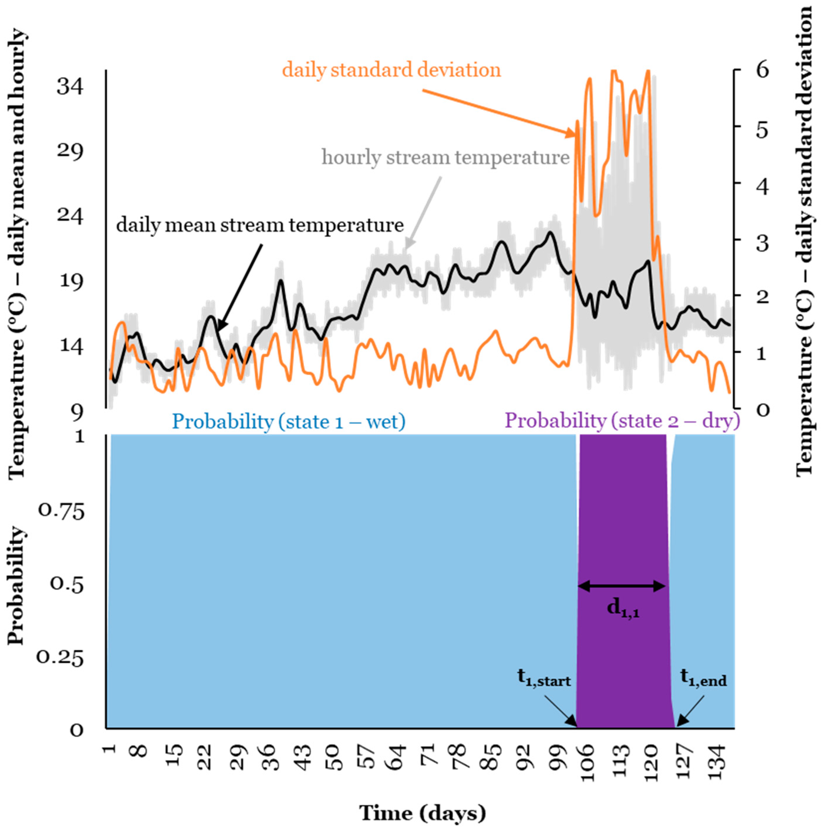
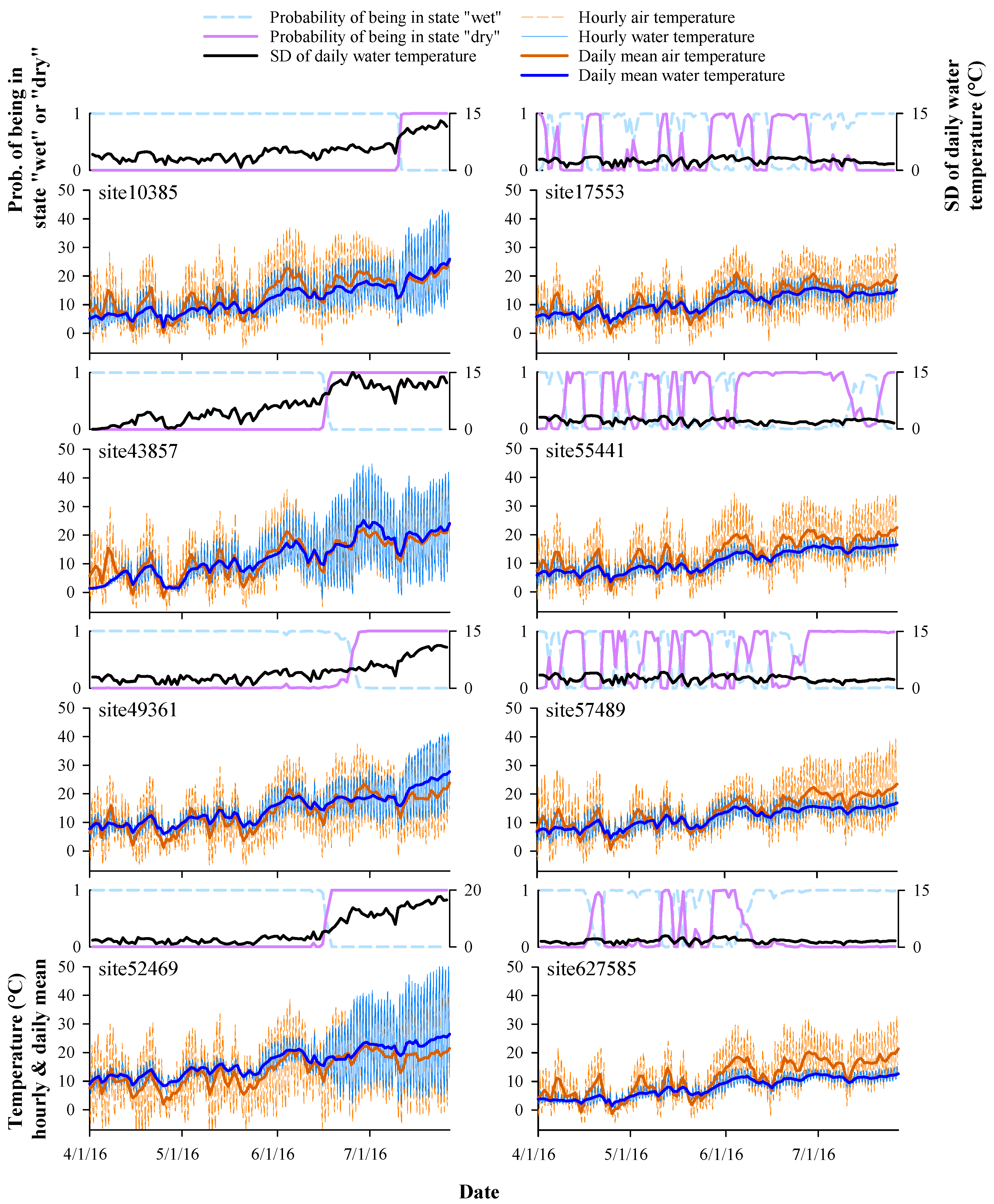
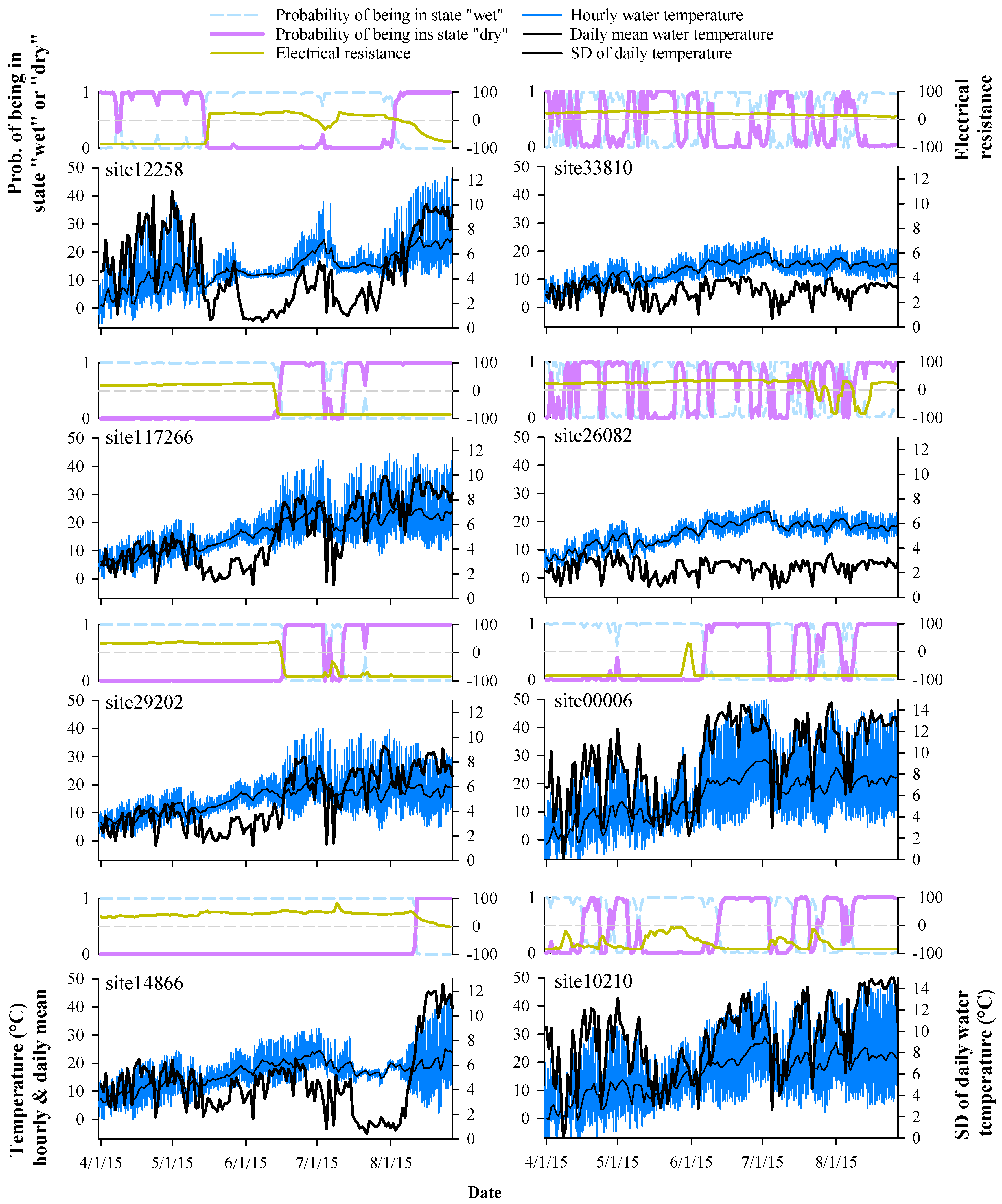
2.2. Statistical Analyses
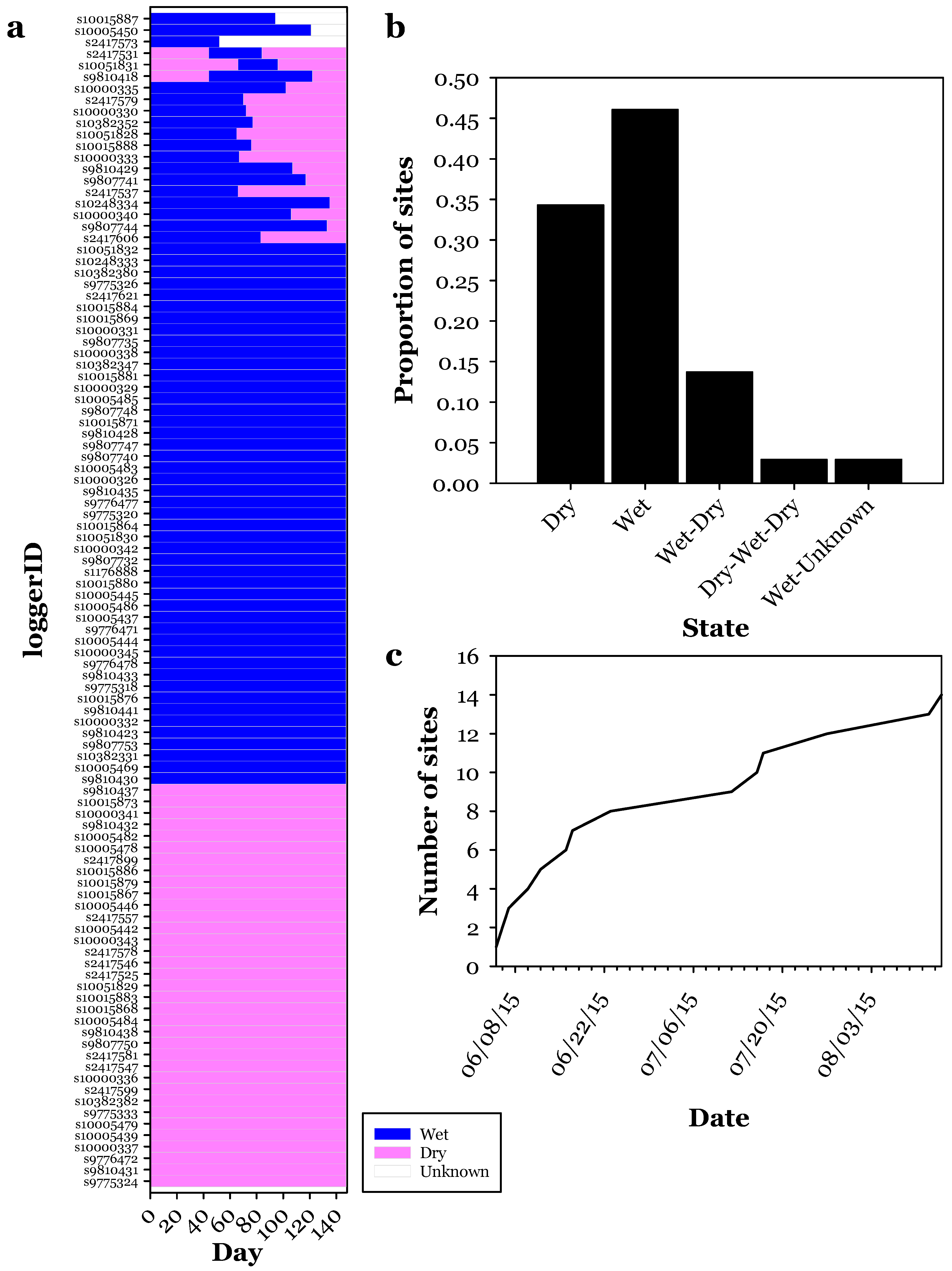
3. Results
4. Discussion
Acknowledgments
Author Contributions
Conflicts of Interest
References
- Jaeger, K.L.; Olden, J.D.; Pelland, N.A. Climate change poised to threaten hydrologic connectivity and endemic fishes in dryland streams. Proc. Natl. Acad. Sci. USA 2014, 38, 13894–13899. [Google Scholar] [CrossRef] [PubMed]
- Datry, T.; Arscott, D.B.; Sabater, S. Recent perspectives on temporary river ecology. Aquat. Sci. 2011, 73, 453–457. [Google Scholar] [CrossRef]
- Morisawa, M.E. Accuracy of determination of stream lengths from topographic maps. Eos Trans. AGU 1957, 38, 86–88. [Google Scholar] [CrossRef]
- Fritz, K.M.; Hagenbuch, E.; D’Amico, E.; Reif, M.; Wigington, P.J., Jr.; Leibowitz, S.G.; Comeleo, R.L.; Ebersole, J.L.; Nadeau, T. Comparing the Extent and Permanence of Headwater Streams from Two Field Surveys to Values from Hydrographic Databases and Maps. J. Am. Water Resour. Assoc. 2013, 49, 867–882. [Google Scholar] [CrossRef]
- Sando, R.; Blasch, K.W. Predicting alpine headwater stream intermittency: A case study in the northern Rocky Mountains. Ecohydrol. Hydrobiol. 2015, 15, 68–80. [Google Scholar] [CrossRef]
- Constantz, J.; Stonestrom, D.; Stewart, A.E.; Niswonger, R.; Smith, T.R. Analysis of streambed temperatures in ephemeral channels to determine streamflow frequency and duration. Water Resour. Res. 2001, 37, 317–328. [Google Scholar] [CrossRef]
- Bhamjee, R.; Lindsay, J.B. Ephemeral stream sensor design using state loggers. Hydrol. Earth Syst. Sci. 2011, 15, 1009–1021. [Google Scholar] [CrossRef]
- Isaak, D.J.; Wenger, S.J.; Peterson, E.E.; Ver Hoef, J.M.; Hostetler, S.W.; Luce, C.H.; Dunham, J.B.; Kershner, J.L.; Roper, B.B.; Nagel, D.E.; et al. NorWeST Modeled Summer Stream Temperature Scenarios for the Western U.S. Fort Collins, CO. For. Serv. Res. Data Arch. 2016. [Google Scholar] [CrossRef]
- Sowder, C.; Steel, E.A. A note on the collection and cleaning of water temperature data. Water 2012, 4, 597–606. [Google Scholar] [CrossRef]
- Blasch, K.W.; Ferré, T.; Hoffman, J.P. A statistical technique for interpreting streamflow timing using streambed sediment thermographs. Vadose Zone J. 2004, 3, 936–946. [Google Scholar] [CrossRef]
- Dunham, J.B.; Chandler, G.L.; Rieman, B.E.; Martin, D. Measuring Stream Temperature with Digital Data Loggers: A User’s Guide; Rocky Mountain Research Center General Technical Report RMRS-GTR-150WWW; U.S. Dep. Agric., Forest Service: Fort Collins, CO, USA, 2005. [CrossRef]
- Zucchini, W.; MacDonald, I. Hidden Markov Models for Time Series: An Introduction Using R, 1st ed.; CRC Press: Boca Raton, FL, USA, 2009; ISBN 978-1-58488-573-3. [Google Scholar]
- Blasch, K.W.; Ferré, T.; Christensen, A.H.; Hoffman, J.P. New field method to determine streamflow timing using electrical resistance sensors. Vadose Zone J. 2002, 1, 289–299. [Google Scholar] [CrossRef]
- Schultz, L.D.; Heck, M.P.; Hockman-Wert, D.; Allai, T.; Wenger, S.; Cook, N.A.; Dunham, J.B. Spatial and temporal variability in the effects of wildfire and drought on thermal habitat for a desert trout. J. Arid Environ. 2017, 145, 60–68. [Google Scholar] [CrossRef]
- Heck, M.P.; Schultz, L.D.; Hockman-Wert, D.; Dinger, E.; Dunham, J.B. Monitoring stream temperatures: A guide for non-specialists. 2017; manuscript in preparation. [Google Scholar]
- Chapin, T.P.; Todd, A.S.; Zeigler, M.P. Robust, low-cost data loggers for stream temperature, flow intermittency, and relative conductivity monitoring. Water Resour. Res. 2014, 50, 6542–6548. [Google Scholar] [CrossRef]
- Visser, I. Seven things to remember about hidden Markov models: A tutorial on Markovian models for time series. J. Math. Psychol. 2011, 55, 403–415. [Google Scholar] [CrossRef]
- Visser, I.; Speekenbrink, M. depmixS4: An R Package for Hidden Markov Models. J. Stat. Softw. 2010, 36, 1–21. [Google Scholar] [CrossRef]
- R Development Core Team. R: A Language and Environment for Statistical Computing; R Foundation for Statistical Computing: Vienna, Austria, 2011; ISBN 3-900051-07-0. [Google Scholar]
- Bhamjee, R.; Lindsay, J.B.; Cockburn, J. Monitoring ephemeral headwater streams: A paired sensor approach. Hydrol. Process. 2016, 30, 888–898. [Google Scholar] [CrossRef]
- Gungle, B. Timing and Duration of Flow in Ephemeral Streams of the Sierra Vista Subwatershed of the Upper San Pedro River Basin, Cochise County, Southeastern Arizona; Scientific Investigations Report 2005–5190, Govt. Doc. Number I 19.42/4-4:2005-5190; United States Geological Survey: Reston, VA, USA, 2006.
- Arismendi, I.; Johnson, S.L.; Dunham, J.B. Technical Note: Higher-order statistical moments and a procedure that detects potentially anomalous years as two alternative methods describing alterations in continuous environmental data. Hydrol. Earth Syst. Sci. 2015, 11, 1169–1180. [Google Scholar] [CrossRef]
- Acuña, V.; Datry, T.; Marshall, J.; Barcelo, D.; Dahm, C.N.; Ginebreda, A.; McGregor, G.; Sabater, S.; Tockner, K.; Palmer, M.A. Why should we care about temporary waterways? Science 2014, 343, 1080–1081. [Google Scholar] [CrossRef] [PubMed]
- Meinzer, O.E. Plants as Indicators of Groundwater; Water Supply Paper 577; United States Geological Survey: Washington, DC, USA, 1927. Available online: https://pubs.usgs.gov/wsp/0577/report.pdf (accessed on 2 December 2017).
- Botter, G.; Zanardo, S.; Porporato, A.; Rodriguez-Iturbe, I.; Rinaldo, A. Ecohydrological model of flow duration curves and annual minima. Water Resour. Res. 2008, 44, W08418. [Google Scholar] [CrossRef]
- Iacobellis, V. Probabilistic model for the estimation of T year flow duration curves. Water Resour. Res. 2008, 44, W02413. [Google Scholar] [CrossRef]
- Pumo, D.; Viola, F.; La Loggia, G.; Noto, L.V. Annual flow duration curves assessment in ephemeral small basins. J. Hydrol. 2014, 519, 258–270. [Google Scholar] [CrossRef]
- Diffenbaugh, N.S.; Swain, D.L.; Touma, D. Anthropogenic warming has increased drought risk in California. Proc. Natl. Acad. Sci. USA 2015, 112, 3931–3936. [Google Scholar] [CrossRef] [PubMed]


© 2017 by the authors. Licensee MDPI, Basel, Switzerland. This article is an open access article distributed under the terms and conditions of the Creative Commons Attribution (CC BY) license (http://creativecommons.org/licenses/by/4.0/).
Share and Cite
Arismendi, I.; Dunham, J.B.; Heck, M.P.; Schultz, L.D.; Hockman-Wert, D. A Statistical Method to Predict Flow Permanence in Dryland Streams from Time Series of Stream Temperature. Water 2017, 9, 946. https://doi.org/10.3390/w9120946
Arismendi I, Dunham JB, Heck MP, Schultz LD, Hockman-Wert D. A Statistical Method to Predict Flow Permanence in Dryland Streams from Time Series of Stream Temperature. Water. 2017; 9(12):946. https://doi.org/10.3390/w9120946
Chicago/Turabian StyleArismendi, Ivan, Jason B. Dunham, Michael P. Heck, Luke D. Schultz, and David Hockman-Wert. 2017. "A Statistical Method to Predict Flow Permanence in Dryland Streams from Time Series of Stream Temperature" Water 9, no. 12: 946. https://doi.org/10.3390/w9120946
APA StyleArismendi, I., Dunham, J. B., Heck, M. P., Schultz, L. D., & Hockman-Wert, D. (2017). A Statistical Method to Predict Flow Permanence in Dryland Streams from Time Series of Stream Temperature. Water, 9(12), 946. https://doi.org/10.3390/w9120946