Article

Evaluation of the Oh, Dubois and IEM Backscatter Models Using a Large Dataset of SAR Data and Experimental Soil Measurements

1
Irstea (Institut National de Recherche en Sciences et Technologies pour l’Environnement et l’Agriculture), UMR-TETIS (Unité Mixte de Recherche, Territoires, Environnement, Télédétection et Information Spatiale), 500 rue François Breton, F-34093 Montpellier CEDEX 5, France
2
CESBIO (Centre d’Etudes Spatiales de la BIOsphère), 18 av. Edouard Belin, bpi 2801, 31401 Toulouse CEDEX 9, France
3
CNR-IFAC (National Research Council, Institute of Applied Physics), via Madonna del Piano 10, Sesto Fiorentino, 50019 Firenze, Italy
4
Laboratory of Hydrology and Water Management, Ghent University, B-9000 Ghent, Belgium
5
Global Modeling and Assimilation Office, NASA Goddard Space Flight Center, Greenbelt, MD 20771, USA
6
CNR-ISSIA (Consiglio Nazionale delle Ricerche, Istituto di Studi sui Sistemi Intelligenti per l’Automazione), via Amendola 122/D, 70126 Bari, Italy
*
Author to whom correspondence should be addressed.
Water 2017, 9(1), 38; https://doi.org/10.3390/w9010038
Submission received: 15 November 2016 / Revised: 28 December 2016 / Accepted: 3 January 2017 / Published: 11 January 2017
(This article belongs to the Special Issue Remote Sensing of Soil Moisture)

Abstract

:
The aim of this paper is to evaluate the most used radar backscattering models (Integral Equation Model “IEM”, Oh, Dubois, and Advanced Integral Equation Model “AIEM”) using a wide dataset of SAR (Synthetic Aperture Radar) data and experimental soil measurements. These forward models reproduce the radar backscattering coefficients ( σ 0 ) from soil surface characteristics (dielectric constant, roughness) and SAR sensor parameters (radar wavelength, incidence angle, polarization). The analysis dataset is composed of AIRSAR, SIR-C, JERS-1, PALSAR-1, ESAR, ERS, RADARSAT, ASAR and TerraSAR-X data and in situ measurements (soil moisture and surface roughness). Results show that Oh model version developed in 1992 gives the best fitting of the backscattering coefficients in HH and VV polarizations with RMSE values of 2.6 dB and 2.4 dB, respectively. Simulations performed with the Dubois model show a poor correlation between real data and model simulations in HH polarization (RMSE = 4.0 dB) and better correlation with real data in VV polarization (RMSE = 2.9 dB). The IEM and the AIEM simulate the backscattering coefficient with high RMSE when using a Gaussian correlation function. However, better simulations are performed with IEM and AIEM by using an exponential correlation function (slightly better fitting with AIEM than IEM). Good agreement was found between the radar data and the simulations using the calibrated version of the IEM modified by Baghdadi (IEM_B) with bias less than 1.0 dB and RMSE less than 2.0 dB. These results confirm that, up to date, the IEM modified by Baghdadi (IEM_B) is the most adequate to estimate soil moisture and roughness from SAR data.

1. Introduction

In the context of sustainable development, soil and water resources management is a key issue not only from the environmental point of view, but also from a socioeconomic perspective [1]. Soil surface characteristics (SSC), such as moisture (mv), roughness, texture, and slaking crusts are some key variables used to understand and model natural hazards, such as erosion, drought, runoff, and floods [2]. Particularly, soil moisture and roughness are important variables in land surface hydrology as they control the amount of water that infiltrates into the soil and replenishes the water table [3]. Synthetic Aperture Radar (SAR) data were widely and successfully used for monitoring the spatial and temporal evolution of soil moisture and roughness [4,5,6,7]. The estimation of soil moisture and roughness was performed by inverting the measured SAR backscatter through SAR backscattering models (both empirical and physical). Unlike physical models, empirical models need to be calibrated using site specific in situ measurements and SAR observation at each time are used over a different study area. Moreover, the validity domain of semi-empirical models is limited to the range of data used for calibration. The most commonly empirical models are the models of Oh [8,9,10,11] and Dubois [12]; while, the most popular physical models are Integral equation model (IEM) [13], IEM calibrated by Baghdadi, called in this paper “IEM_B” [14,15,16,17,18,19], and Advanced Integral Equation Model (AIEM) [20].
For bare soils, SAR backscattering models allow backscattering coefficients simulation by using soil parameters (mainly dielectric constant, and roughness) and SAR configurations (frequency, incidence angle, polarization) as input. Several studies reported important discrepancies between backscattering models simulations and SAR observations [15,21,22,23]. The discrepancy between SAR simulations and SAR measurements is mainly related to the description of surface roughness which is an important input to SAR backscattering models [17,24,25]. For most of the backscattering models the surface roughness is described by three parameters: the standard deviation of the height (Hrms), the correlation length (L) and the shape of the correlation function [13,26]. The correlation length is usually measured with an uncertainty which introduces an error on simulated backscattering coefficients [27,28,29,30,31,32,33]. A few studies proposed a semi-empirical calibration of SAR backscattering models in order to reduce the uncertainty on SAR simulations [14,15,16,17,18,19,34]. In [14,15,16,17,18,19] the method consisted of replacing the measured L by a fitting parameter, so-called Lopt, which was found to be related to Hrms (Lopt increases with Hrms). Lopt is a function of Hrms (linear, exponential, or power calibration) which depends on SAR parameters (incidence angle, polarization and frequency). This calibration reduces IEM’s input soil parameters (Hrms and mv instead of Hrms, L and mv). Rahman et al. [34] proposed a method for deriving L through the IEM. In this method, the radar signal is modeled as a function of only Hrms and L, and the contribution of soil moisture on backscattering coefficients is ignored (dry soil). Thus, L could be estimated by inverting the IEM.
Several studies have been carried out to evaluate and compare the robustness of the backscattering models such as, Oh, Dubois and IEM (original IEM, IEM_B and AIEM). Zribi et al. [23] evaluated the Oh model and IEM using L-, C- and X-bands SAR data and in situ measurements. Results showed that the IEM provides accurate simulations (RMSE about 2.0 dB) only over smooth surfaces. In addition, for rough surfaces and medium incidence angle, Oh model simulations retrieve backscattering values very close to the measured ones, while showing poor correlation with measured backscattering coefficients over smooth areas. Baghdadi and Zribi [21] evaluated the backscattering models IEM, Oh and Dubois by using large C-band SAR data and in situ measurements. Results showed that these models frequently tend to over-estimate or under-estimate the radar signal (in the order of −3.0 dB) and the errors on model simulation depend on height surface roughness, Hrms, soil moisture, mv, and/or incidence angle. Baghdadi et al. [18] evaluated the potential of IEM, Oh and Dubois models by using TerraSAR-X images acquired over France and Tunisia and experimental datasets of in situ measurements (mv ranged between 5 vol. % and 41 vol. % and Hrms between 0.42 cm and 4.55 cm). In this case, the semi-empirical Oh model correctly simulated the backscattering (showing over or under-estimation of the backscatter <1 dB, and RMSE <3 dB), while Dubois model showed a poor correlation between real data and simulations, with RMSE between 2.2 and 4.4 dB and over or under-estimation of the backscatter of about 3.4 dB. In addition, the IEM simulates correctly the backscattering at X-band for Hrms < 1.5 cm by using the exponential correlation function and for Hrms > 1.5 cm by using the Gaussian correlation function. Panciera et al. [35] compared the performances of the IEM, Dubois and Oh models by using fully polarized L-band airborne data (incidence angles between 24° and 38°) and in situ measurements (mv between 5 vol. % and 39 vol. % and Hrms between 1 cm and 7.6 cm) acquired over the study area in southeastern Australia. At HH polarization, the three models simulated the backscattering with almost similar accuracy, showing a mean error between the simulated and the observed backscattering coefficients of about 1.6 dB in absolute value (standard deviation “std” about ±2.5 dB). At VV polarization, the Oh model resulted to be more accurate than IEM and Dubois models: the mean errors between the simulated and observed backscattering were equal to 4.5 dB (std = ±2.0 dB), 1.7 dB (std = ±2.3 dB), and −0.4 dB (std = ±2.4 dB) for IEM, Dubois, and Oh model, respectively.
Several studies confirmed that the use of the calibrated correlation length, as proposed by Baghdadi et al. [14,15,16,17,18,19] is able to improves the performance of the IEM at both both HH and VV polarizations [35,36,37]. Dong et al. [36] used the calibrated correlation length in the AIEM to simulate SAR data in C-band. Results showing that the RMSE reduced from 3.1 to 1.7 dB at HH and VV polarizations and from 31.0 to 5.1 dB at HV polarization. Panciera et al. [35] showed that the use of calibrated correlation length decreases the errors on IEM simulation with a bias equal to about −0.3 dB (std about ±1.1 dB) at both HH and VV polarizations.
The aim of this study is to evaluate the most popular backscattering SAR models (Oh, Dubois, IEM, IEM_B, and AIEM) by using a wide range of SAR data and in situ measurements. With the arrival of Sentinel-1A and -1B satellites that provide free high resolution SAR data with 3 days revisit time, several research teams work actually on developing methods for mapping soil moisture using these Sentinel-1 data. Most of methods for soil moisture mapping are based on backscatter models for soil moisture estimations. The objective of our study is to evaluate the most commonly backscatter models using a wide dataset of SAR data and in situ measurements acquired over numerous agricultural sites in France, Italy, Germany, Belgium, Luxembourg, Canada and Tunisia. Thus, this study could be of a great importance for scientific community since it help on understand backscatter models performance for wide range of soil surface conditions, acquired for several study areas through the world by numerous SAR sensors. Never before have been evaluated all these backscatter models together in the same literature with such a wide dataset. In addition, this study is the first that evaluates the backscatter models using L-, C- and X-bands together. A description of the study areas and different datasets used in this study is provided in Section 2. Section 3 the models are described. The results are shown in Section 4. Finally, Section 5 presents the conclusion.

2. Dataset

2.1. Study Areas

A wide range of datasets composed of AIRSAR, SIR-C, JERS-1, PALSAR-1, ESAR, ERS, RADARSAT, ASAR and TerraSAR-X acquisitions over numerous agricultural sites in France, Italy, Germany, Belgium, Luxembourg, Canada and Tunisia (Table 1), have been used in this research work. In addition, in situ measurements of soil moisture and surface roughness were carried out simultaneously to SAR acquisitions over bare soil surfaces.

2.2. Satellite Data

A large number of L-, C- and X-band images (approximately 1.25 GHz, 5.3 GHz and 9.6 GHz, respectively) were acquired between 1994 and 2014 with different incidence angles (between 18° and 57°) and in HH, VV and HV polarizations (Table 1). The spatial resolution of SAR images is between 1 m and 30 m (Table 1). Images were first radiometrically calibrated to enable the extraction of the backscattering coefficients ( σ 0 ). Then, the mean backscattering coefficients were computed from calibrated SAR images by linearly averaging the σ 0 values of all pixels within the plot.

2.3. Field Data

Field measurements of soil moisture and surface roughness have been collected from bare plots selected over the study areas. Each plot is a homogeneous surface (similar soil type, moisture content and surface roughness) of around one hectare or more. In situ measurements of soil moisture (mv, in vol. %) were carried out for a soil layer of 5 cm or 10 cm in each reference plot by using both the gravimetric method or a calibrated TDR (time domain reflectometry) probe. For each bare soil reference field the average soil moisture (mv) of all samples was calculated. The soil moisture ranged between 2 vol. % and 47 vol. %.
Roughness measurements were carried out by using laser or needle profilometers (mainly 1 m and 2 m long, and with 1 cm and 2 cm sampling intervals); while for some in situ measurement campaigns, a meshboard technique was used. Several roughness profiles along and across the direction of tillage were acquired in each reference field. The standard deviation of surface heights (Hrms) and the correlation length (L) were calculated by using the mean of all experimental correlation functions. In our dataset, Hrms ranged from 0.2 cm to 9.6 cm and the L from 1.2 cm to 38.5 cm.
A total of 2442 experimental data of soil moisture content and surface roughness were available, together with the corresponding values of backscattering coefficient, of which 1262 at HH polarization, 790 at VV polarization, and 390 at HV polarization (see Table 1).

3. Description of the Backscattering Models

3.1. The Semi-Empirical Dubois Model

Dubois et al. [12] proposed a semi-empirical model for simulating the backscattering coefficients in HH and VV polarizations ( σ H H 0 and σ V V 0 ) on bare soils. The expression of σ H H 0 and σ V V 0 depends on the incident angle (θ), the soil dielectric constant (ε, which is a function of the soil moisture content), the soil roughness defined by the standard deviation of surface height (Hrms), and the radar wavelength (λ = 2π/k where k is the wave number). The model optimized for bare soils according to the validity domain defined by kHrms ≤ 2.5, mv ≤ 35 vol. %, and θ ≥ 30° is expressed as:
σ V V 0 = 10 2.35 ( cos 3 θ sin 3 θ )    10 0.046 ε tan θ ( k H r m s sin θ ) 1.1 λ 0.7 σ H H 0 = 10 2.75 ( cos 1.5 θ sin 5 θ )    10 0.028 ε tan θ ( k H r m s sin θ ) 1.4 λ 0.7
where θ is expressed in radians and λ in cm, and σ H H 0 and σ V V 0 are expressed in linear units.

3.2. The Semi-Empirical Oh Model

Oh et al. [8,9,10,11] developed between 1992 and 2004 several versions of a semi empirical backscattering model. Basing on theoretical models, scatterometer measurements and airborne SAR observations, the Oh model is built over a wide variety of bare soil surfaces. The Oh model relates the co-polarized ratio p (= σ H H 0 / σ V V 0 ) and the cross-polarized ratio q (= σ H V 0 / σ V V 0 ) to incident angle (θ), wave number (k), standard deviation of surface height (Hrms), correlation length (L), and soil moisture (mv) or dielectric constant ( ε r ).
The initial version of the Oh model [9] is defined as:
p = σ H H 0 σ V V 0 = [ 1 ( θ 90 ) 1 3 Γ 0 . e k H r m s ] 2
q = σ H V 0 σ V V 0 = 0.23 Γ 0 ( 1 e k H r m s )
where:
Γ 0 = | 1 ε r 1 + ε r | 2
Oh et al. [10] proposed a new expression for q to incorporate the effect of the incidence angle:
q = σ H V 0 σ V V 0 = 0.25 Γ 0 ( 0.1 + sin 0.9 θ ) ( 1 e [ 1.4 1.6 Γ 0 ] k H r m s )
Oh et al. [11] again modified the expressions for p and q, and the following expression for the cross-polarized backscatter coefficient was proposed:
p = σ H H 0 σ V V 0 = 1 ( θ 90 ) 0.35 m v 0.65 . e 0.4 ( k H r m s ) 1.4
q = σ H V 0 σ V V 0 = 0.1 ( H r m s L + sin 1.3 θ ) 1.2 ( 1 e 0.9 ( k H r m s ) 0.8 )
σ H V 0 = 0.11 m v 0.7 cos 2.2 θ ( 1 e 0.32 ( k H r m s ) 1.8 )
Oh and Kay [51] demonstrated that the measurement of the correlation length is not accurate and that the ratio q is not sensitive to the roughness parameter (defined as Hrms/L). Thus, Oh [8] proposed a new equation for q that ignores the correlation length (L):
q = σ H V 0 σ V V 0 = 0.095 ( 0.13 + sin 1.5 θ ) 1.4 ( 1 e 1.3 ( k H r m s ) 0.9 )
The Oh model [8] is optimized for bare soils in the following validity domain: 0.13 ≤ kHrms ≤ 6.98, 4 ≤ mv (vol. %) ≤ 29.1, and 10° ≤ θ ≤ 70°.
The estimation of soil moisture and surface roughness from Oh model requires two backscattering coefficients at least, with one co-polarized coefficient ( σ H H 0 or σ V V 0 ) and one cross-polarized coefficient ( σ H V 0 or σ V H 0 ). The availability of σ V V 0 and σ V H 0 allows using the ratio q and σ H V 0 in the inversion process of SAR data, while the ratio p/q, as well as σ H V 0 , is used in the case where SAR data are available in the both HH and HV polarizations.

3.3. The Physical Integral Equation Model (IEM)

The Integral Equation IEM is a physical model [13], where the soil is characterized by the dielectric constant ( ε r ), the standard deviation of surface height (Hrms), the form of the correlation function, and the correlation length (L). The IEM also takes into account the sensor parameters such as the incidence angle (θ), the polarization (pq with p,q = H or V), and the radar wave number (k = 2π/λ where λ is the wavelength). The IEM has a validity domain that covers the range of roughness values that are commonly encountered for agricultural surfaces:
k H r m s     3 ( ( k H r m s cos θ ) 2 / 0.46 k L )    exp { 0.92 k L ( 1 sin θ ) } < 0.25
Over bare soils in agricultural areas, the backscattering coefficient of the surface contribution is expressed at HH and VV polarizations as:
σ p p 0 = k ² 2 | f p p | 2 e 4 k 2 H r m s 2 cos 2 θ n = 1 + ( 4 k 2 H r m s 2 cos 2 θ ) n n !    W ( n ) ( 2 k sin θ , 0 )     + k ² 2 Re ( f p p * F p p ) e 3 k 2 H r m s 2 cos 2 θ n = 1 + ( 4 k 2 H r m s 2 cos 2 θ ) n n ! W ( n ) ( 2 k sin θ , 0 )     + k ² 8 | F p p | 2 e 2 k 2 H r m s 2 cos 2 θ n = 1 + ( k 2 H r m s 2 cos 2 θ ) n n ! W ( n ) ( 2 k sin θ , 0 )
At cross polarization, the backscattering coefficient is as follows:
σ h v 0 = k ² 16 π e 2 k 2 H r m s 2 cos 2 θ n = 1 + m = 1 + ( k 2 H r m s 2 cos 2 θ ) n + m n ! m !    [ | F h v ( u , v ) | 2 + F h v ( u , v ) F h v * ( u , v ) ]    W ( n ) ( u k sin θ , v ) W ( m ) ( u + k sin θ , v ) d u d v
where:
f h h = 2 R h cos θ ; f v v = 2 R v cos θ
R h = μ r cos θ μ r ε r sin 2 θ μ r cos θ + μ r ε r sin 2 θ Fresnel   coefficient   at   horizontal   polarization
R v = ε r cos θ μ r ε r sin 2 θ ε r cos θ + μ r ε r sin 2 θ Fresnel   coefficient   at   vertical   polarization
F h h = 2 sin 2 θ cos θ [ 4 R h ( 1 1 ε r ) ( 1 + R h ) 2 ]
F v v = 2 sin 2 θ cos θ [ ( 1 ε r cos 2 θ μ r ε r sin 2 θ ) ( 1 R v ) 2 + ( 1 1 ε r ) ( 1 + R v ) 2 ]
F h v ( u , v ) = u v k cos θ [ 8 R 2 k 2 u 2 v 2 + 2 + 6 R 2 + ( 1 + R ) 2 ε r + ε r ( 1 R ) 2 ε r k 2 u 2 v 2 ]
R = R v R h 2
ε r : dielectric constant, obtained on the basis of volumetric water content (mv). In our study, Hallikainen empirical model is used [52].
μ r : relative permittivity.
Re: real part of the complex number.
f p p * : conjugate of the complex number f p p .
W ( n ) is the Fourier transform of the nth power of the surface correlation ρ ( x , y ) function:
W ( n ) ( a , b ) = 1 2 π ρ n ( x , y ) e i ( a x + b y ) d x d y
The distribution of ρ ( x , y ) is exponential for low surface roughness values and Gaussian for high surface roughness values. For one-dimensional roughness profiles, the correlation functions are defined as follows:
ρ ( x ) = e ( x L )      : exponential    = e ( x L ) 2 : Gaussian

3.4. IEM Modified by Baghdadi (IEM_B)

Several studies reported important discrepancies between backscattering coefficients simulated by IEM and those measured by SAR sensors [23,35,41,46,53,54,55,56]. Baghdadi et al. [14,28] showed that the discrepancy between the observed and IEM simulated backscattering coefficients is mainly due to the correlation length parameter which is difficult to be measured with a good accuracy. To reduce such incongruities between simulated and measured backscattering values, Baghdadi et al. [16,17,19,43] proposed a semi-empirical calibration of the IEM backscattering, which consists of replacing the in situ measured correlation length by a fitting parameter (Lopt). Lopt depends on surface roughness conditions and SAR configurations (incidence angle, polarization and radar wavelength). This calibration has been performed by using large experimental datasets and SAR configurations (incidence angles from 23° to 57°, and HH, HV, and VV polarizations), and it has been carried separately at X-band in [43], C-band in [16,17] and L-band in [19]. The proposed calibration reduces the IEM’s input soil parameters from three to two (Hrms and mv only, instead of Hrms, L and mv).
Lopt is computed at L-, C-, and X-bands using a Gaussian correlation function and it is described as follows:
In   X - band :    { L o p t ( H r m s , θ , H H ) = 18.102 e 1.891 θ   H r m s   0.7644 e 0.2005   θ   L o p t ( H r m s , θ , V V ) = 18.075 e 2.1715 θ   H r m s   1.2594 e 0.8308 θ
In   C - band :    { L o p t ( H r m s , θ , H H ) = 0.162 + 3.006   ( sin 1.23 θ ) 1.494   H r m s L o p t ( H r m s , θ , H V ) = 0.9157 + 1.2289   ( sin 0.1543   θ ) 0.3139   H r m s L o p t ( H r m s , θ , V V ) = 1.281 + 0.134   ( sin 0.19   θ ) 1.59   H r m s
In   L - band :   { L o p   ( H r m s , θ , H H ) = 2.6590   θ 1.4493 + 3.0484   H r m s   θ 0.8044 L o p t ( H r m s , θ , V V ) = 5.8735   θ 1.0814 + 1.3015   H r m s   θ 1.4498
where θ is in radians; Lopt and Hrms are in centimeters. Several studies showed that the use of the fitting parameter Lopt allows more correct estimations of the radar backscattering coefficient [36].

3.5. The Advanced Integral Equation Model

The Advanced Integral Equation Model (AIEM) [20] is the updated version of the Integral Equation Model (IEM) [57]. In a comparison with the IEM, two improvements have been integrated into the AIEM: (1) the complete expressions for the Kirchhoff field coefficient and the complementary field coefficient based on the removal of the simplification assumption of the Green’s function have been included in the AIEM [20] and (2) a continuous Fresnel reflection coefficient is obtained using a transition model [58]. This update allows a more precise calculation of the simple scattering for a surface with a wide range of dielectric constant ( ε r ), large standard deviation of heights Hrms, and various remote sensing configurations. The AIEM simulates the radar backscattering coefficients basing on the same parameters as the IEM.

4. Results and Discussion

This section shows the evaluation results of the five radar backscattering models Dubois, Oh, IEM, IEM_B and AIEM using large datasets, characterized by various radar wavelength (L, C and X), wide range of incidence angles and large geographical distribution in regions with different climate conditions (humid, semi-arid and arid sites). In this study, each plot is considered as a sampling unit. For each plot, SAR data was simulated through backscatter models using in situ measurements (mv, Hrms and L) averaged within that plot. Then, the simulated SAR signal were compared with the backscattering coefficients computed from calibrated SAR images by linearly averaging the σ 0 values of all pixels within the plot.

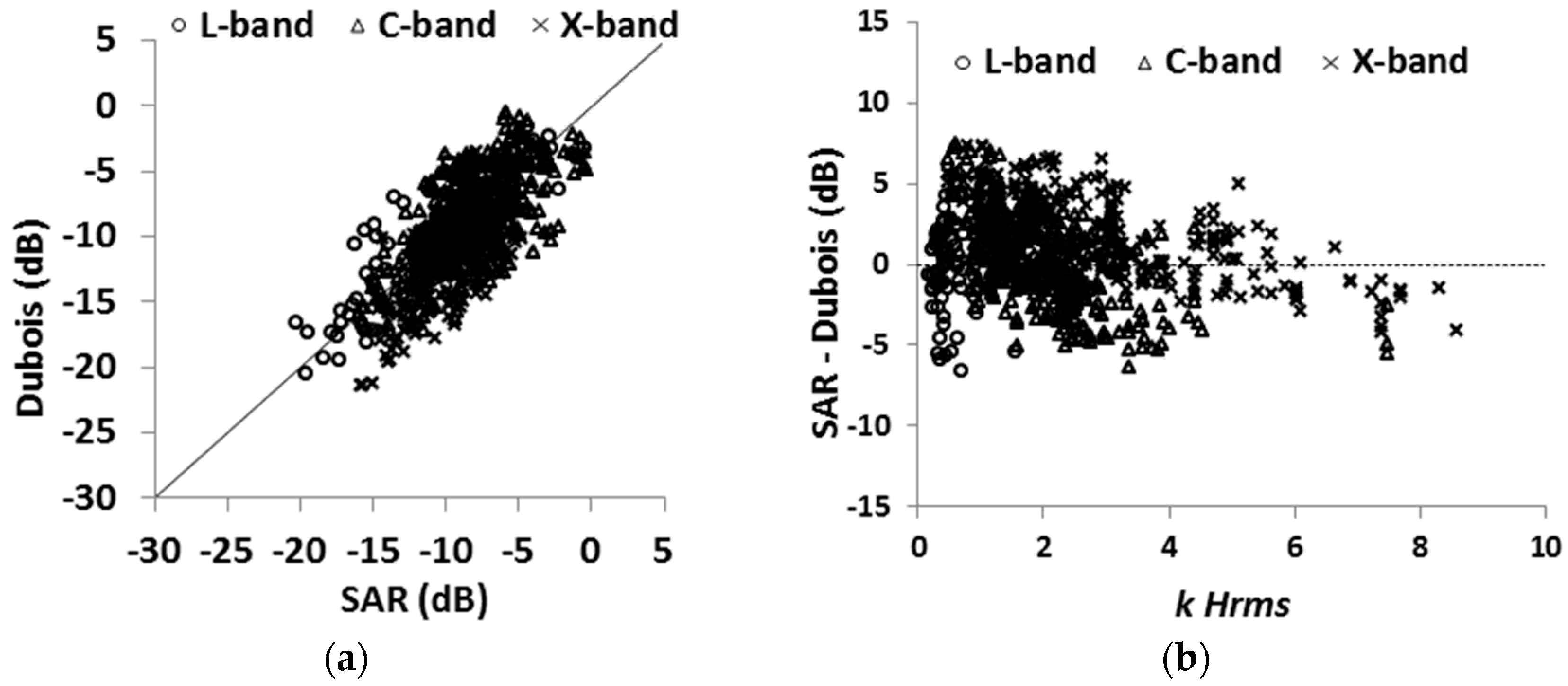
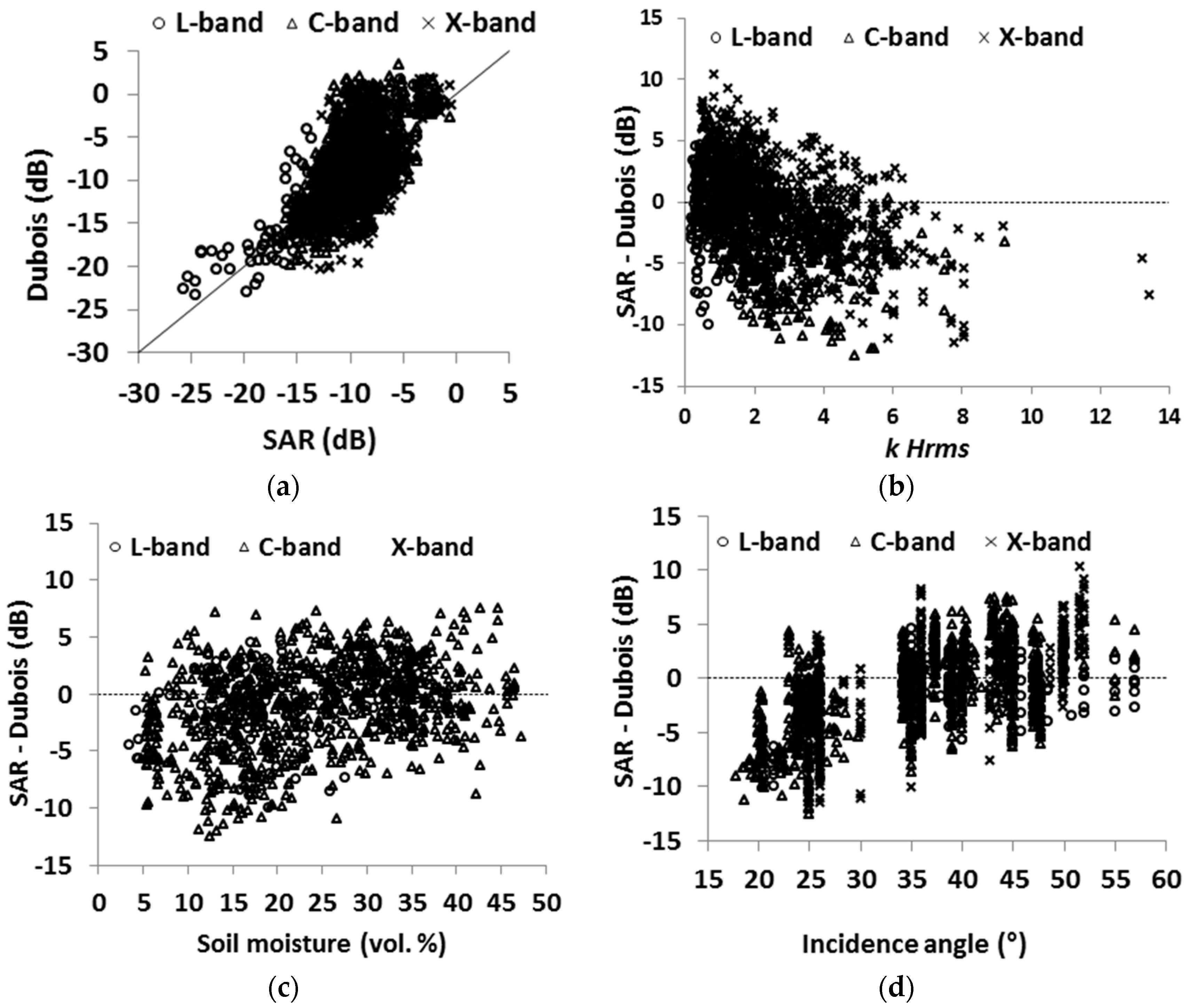
4.1. Evaluation of the Dubois Model

The evaluation of Dubois model was carried out for different scenarios using all data, per radar wavelength, and by range of soil moisture, kHrms, and incidence angle.
Using all data, the Dubois model over-estimates slightly the radar signal by about 1.0 dB in HH polarization and under-estimates slightly the radar signal by about 0.7 dB in VV polarization (Table 2, Figure 1 and Figure 2). RMSE is about 4.0 dB and 2.9 dB at HH and VV polarization, respectively (Table 2). The analysis of the error according to each radar frequency band separately (L, C and X) shows an over-estimation in HH polarization, which is almost the same at L-, C- and X-bands (between 0.9 dB and 1.1 dB). In VV polarization, the Dubois model under-estimates the radar signal by about 1.8 dB and 0.4 dB for X and C bands, respectively. For L band, the Dubois model fits correctly the radar signal in VV because the difference between real data and simulations is about 0.2 dB. The RMSE in HH is the same as at X- and C-bands, and is about 4.1 dB and decreases to 3.0 dB at L-band. In VV polarization, the RMSE increases with the radar frequency (2.5 dB at L-band, 2.8 dB at C-band and 3.1 dB at X-band).
The analysis of the error of the Dubois model according to the validity domain was studied by range of surface roughness (kHrms), soil moisture (mv) and incidence angle (Table 2). The Dubois model underestimates the radar signal for kHrms < 2.5 (validity domain of the Dubois model) by about 0.4 dB and 1.2 dB in HH and VV polarizations, respectively. In the case of kHrms < 2.5, the RMSE is about 3.6 and 3.0 dB for HH and VV polarizations, respectively. In addition, the Dubois model overestimates the radar signal for kHrms > 2.5 by about 2.9 dB in HH polarization with RMSE about 4.6 dB. In VV polarization, the Dubois model fits correctly the radar signal in the case of kHrms > 2.5 with a difference between real and simulated data of about 0.2 dB and a RMSE of 2.5 dB (Table 2).
Moreover, the evaluation of the Dubois model was carried out by range of soil moisture (mv). Results show an overestimation in HH pol. by about 2.6 dB and a slightly underestimation in VV by about 0.5 dB with mv-values lower than 20 vol. % (RMSE = 4.6 and 2.8 dB at HH and VV, respectively) (Table 2). In besides, the Dubois model correctly simulates the backscattering coefficient in HH pol. with a difference between real data and simulations about 0.3 dB and underestimates the radar signal in VV by about 1.0 dB with mv-values greater than 20 vol. %. In the case of mv-values greater than 20 vol. %, the RMSE is about 3.4 dB and 3.0 dB for HH and VV polarization respectively. Finally, the performance of Dubois model was studied according to ranges of incidence angle (Table 2). For θ < 30° (outside the validity domain of the Dubois model), the Dubois model overestimates the radar signal by −4.2 dB in HH polarization (RMSE = 5.5 dB) and slightly underestimates the radar signal in VV polarization (real data − simulations = −0.6 dB) with a RMSE of 2.9 dB. At θ > 30°, the Dubois model correctly simulates the backscattering coefficient in HH pol. with a difference between real data and model of 0.3 dB at HH polarization and underestimates the backscattering at VV pol. by about 1.5 dB (RMSE = 3.2 dB and 2.9 dB for HH and VV polarizations, respectively).

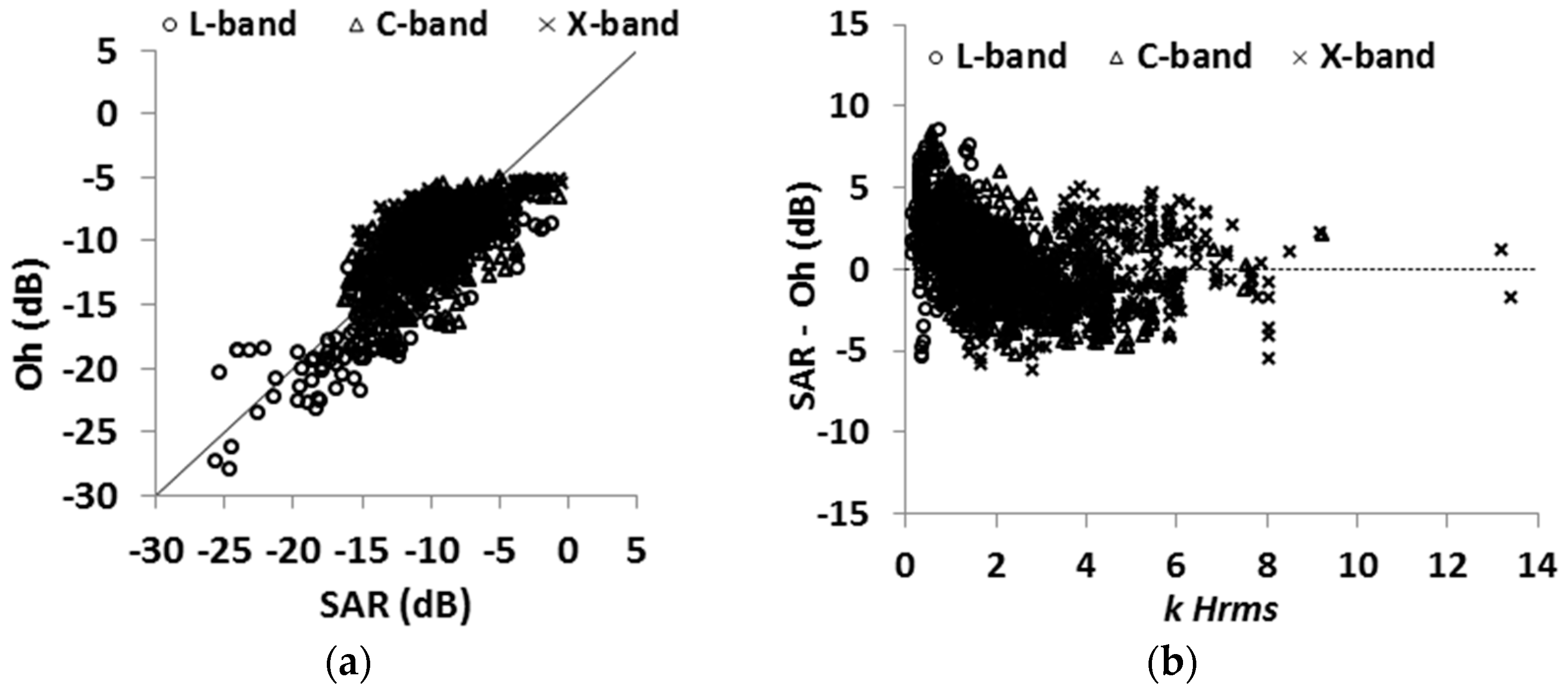
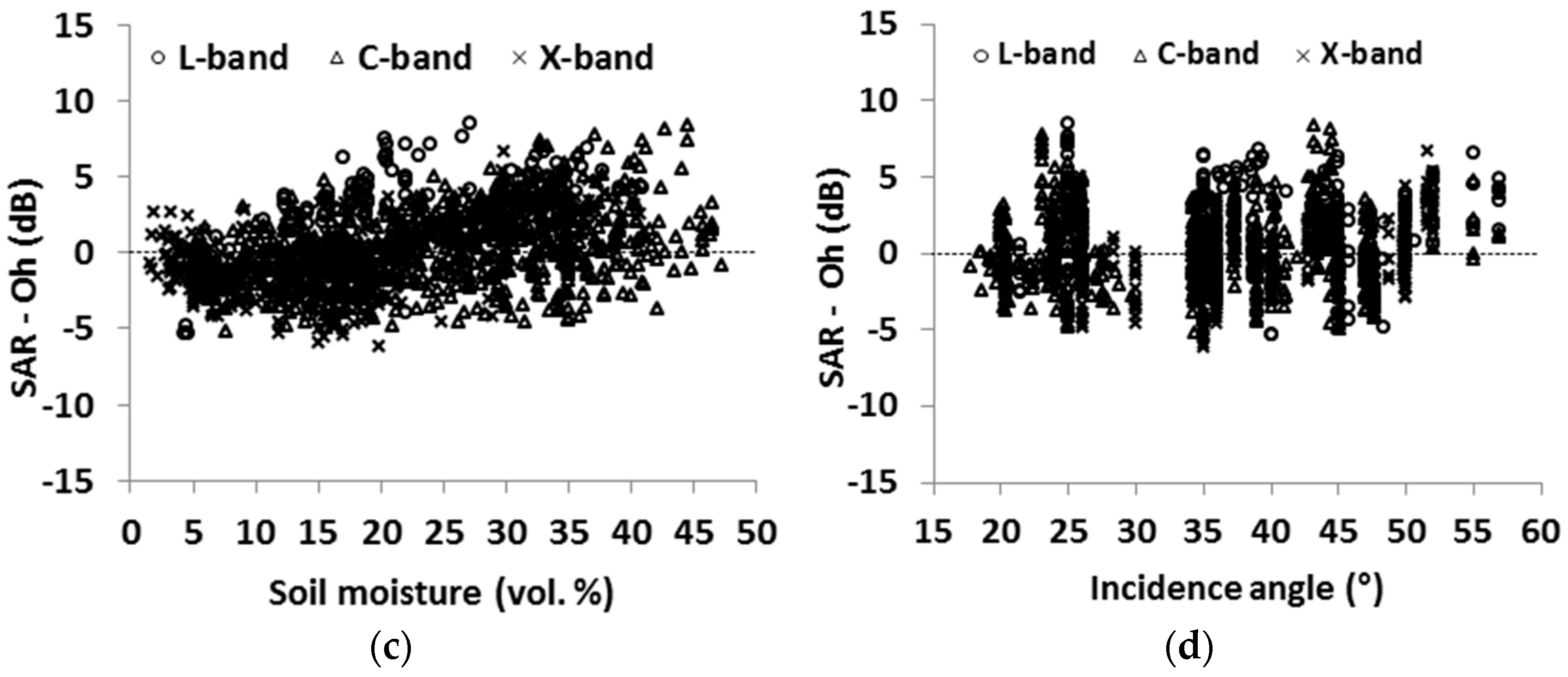
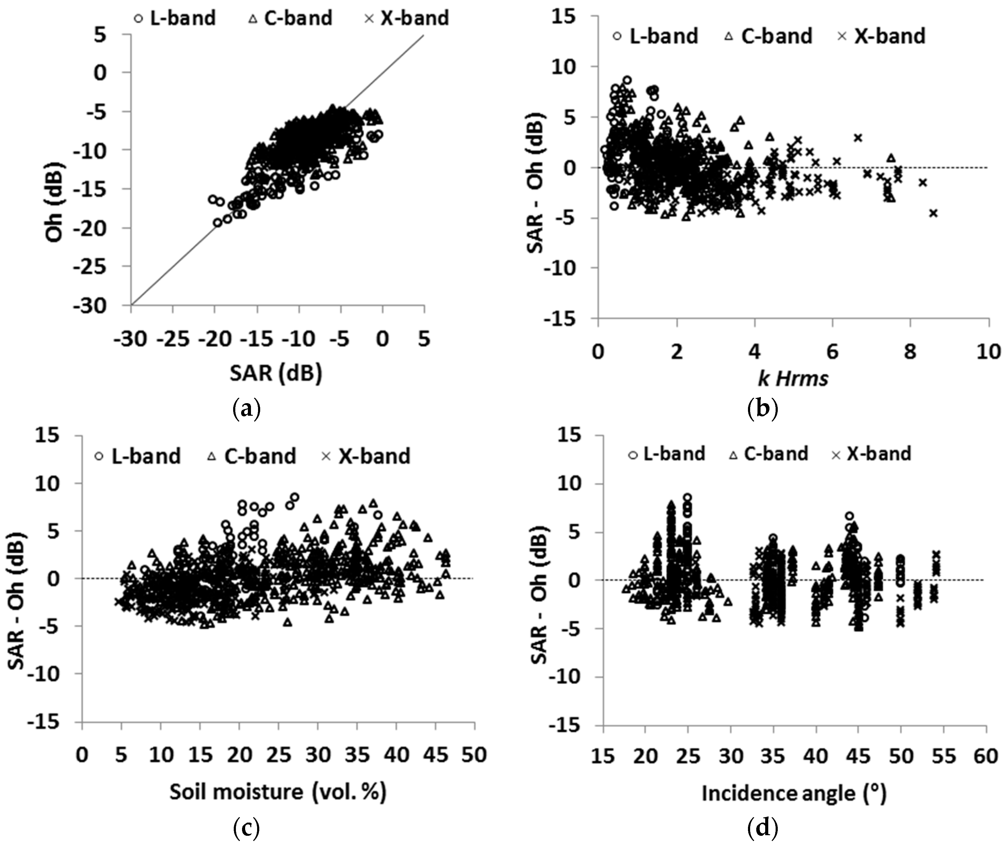
4.2. Evaluation of the Oh Model

The Oh model versions developed in 1992, 1994, 2002 and 2004 were applied to our datasets. The evaluation of the different Oh model versions was carried out firstly using all data, successively for each radar wavelength (L, C and X bands), and finally by range of soil moisture, kHrms and incidence angle (Table 3, Figure 3, Figure 4 and Figure 5).
Using the entire dataset, results showed that the different versions of Oh model correctly simulate the backscattering at both HH and VV polarizations with difference between real data and simulations varying between −0.9 and +0.4 dB at HH pol. and between (−1.3 dB and +0.4 dB) in VV pol. The RMSE values are approximately the same for all models and in both HH and VV polarizations, i.e., between 2.4 dB and 2.8 dB. The Oh 1992 model simulates slightly better the backscattering than the other versions (Table 3). For HV polarization, the Oh 2002 model simulates correctly the backscattering with a difference between real and simulated data of about +0.7 dB, with RMSE equal to 2.9 dB.
In L-band, the different versions of the Oh model underestimate the backscattering at both HH and VV polarizations. This underestimation varies between 1.3 dB and 2.5 dB in HH polarization and between 0.7 dB and 2.1 dB in VV polarization (Table 3). The RMSE is slightly higher in HH than in VV polarization (between 2.8 dB and 3.7 dB in HH and between 2.6 dB and 3.4 dB in VV). The Oh 1994 version better simulates the backscattering than other versions of Oh model, with an underestimation of the backscattering between 1.3 dB and 0.7 dB and RMSE of 2.8 and 2.6 dB for HH and VV polarizations, respectively. At HV polarization, the Oh model underestimates the backscattering by about 1.5 dB with RMSE equal to 3.1 dB.
In C-band, the Oh 1992 model correctly simulates the backscattering in both HH and VV polarizations with differences between real and simulated data of 0.1 dB and 0.4 dB at HH and VV polarizations, respectively (Table 3). Besides, the RMSE is of 2.4 dB at HH and 2.3 dB at VV pol. Moreover, the other Oh versions overestimate the backscattering in both HH and VV polarizations (between 0.9 dB and 1.5 dB) with similar RMSE between 2.6 dB and 2.8 dB. At HV polarization, the Oh 2002 model slightly underestimates the backscattering by about 1.0 dB with a RMSE of 2.7 dB.
The analysis of results obtained in X-band shows that Oh model versions simulate the radar signal with difference between real data and simulations between 0.0 and −1.2 dB in HH and between +0.4 and −2.1 dB in VV (Table 3, Figure 3, Figure 4 and Figure 5). The RMSE is between 2.3 and 2.8 dB in HH and between 2.0 and 2.7 dB in VV polarization. For HV polarization, the Oh model over-estimates the backscattering by about 0.9 dB with RMSE of 3.8 dB.
The analysis of the error was studied by selecting two ranges of surface roughness (kHrms < 2.0 and kHrms > 2.0) (Table 3). This range is different from the general validity domain of the Oh model (0.13 ≤ kHrms ≤ 6.98) because it covers the entire dataset except only a few points. For kHrms < 2.0, the 1994, 2002 and 2004 Oh models simulate correctly the backscattering at both HH and VV polarizations with differences between real data and simulations between −0.5 and +0.6 dB and RMSE between 2.4 dB and 2.7 dB. The Oh 1992 model underestimates the backscattering by 1.3 dB and 1.0 dB at HH and VV polarizations, respectively (RMSE is 2.9 for HH pol. and 2.7 dB for VV pol.). For kHrms > 2.0, the 1992 and 2002 Oh versions simulate correctly backscattering at both HH and VV polarizations with difference between real and simulated data between −0.5 dB and −1.0 dB with RMSE between 2.3 and 2.6 dB. The 1994 Oh model over-estimates the backscattering at both HH and VV polarizations by about 1.7 dB and 2.1 dB, respectively (RMSE = 2.9 dB). The last version of the Oh model (Oh, 2004) underestimates the backscattering in HH polarization by about 1.5 dB (RMSE = 2.6 dB) and over-estimates it in VV polarization by about 2.0 dB (RMSE= 2.8 dB). At HV polarization, for kHrms < 2, the Oh 2002 model underestimates the backscattering in HV by 1.8 dB (RMSE = 2.5 dB). In addition, Oh model correctly fits the backscattering for kHrms > 2.0, with a difference between the real and simulated data of about −0.7 dB and RMSE of 2.5 dB.
Finally, the performance of the Oh model was studied according to its validity domain by selecting two intervals of soil moisture (mv < 29.1 and mv > 29.1 vol. %). For mv < 29.1 vol. %, the 1992 and 2002 Oh versions simulate correctly the backscattering coefficient at both HH and VV polarizations with a difference between real and simulated data varying between −0.3 dB and −0.7 dB. In addition, the 1994 and 2004 Oh models overestimate the backscattering at both HH and VV polarizations (Table 3) with RMSE between 2.6 dB and 2.9 dB. In conclusion, for mv < 29.1 vol. %, the 1992 Oh model provides the best simulations. For mv > 29.1 vol. %, the 1994, 2002 and 2004 Oh models correctly simulate the backscattering with a difference between real and simulated data between −0.8 dB and +0.5 dB, while the 1992 Oh model underestimates the backscattering by about 1.9 dB and 1.5 dB at HH and VV polarizations, respectively (RMSE = 3.1 dB for HH and 2.7 dB for VV). The RMSE values are approximately the same in the Oh 1994, 2002 and 2004 versions, and range between 2.2 dB and 2.6 dB. At HV polarization, the Oh model correctly simulates the backscattering for both range of mv-values, with RMSE of 3.0 dB for mv < 29.1 vol. % and RMSE of 2.6 dB for mv > 29.1 vol. %.
The validity domain of Oh model according to the incidence angle (10° ≤ θ ≤ 70°) covers the entire dataset. Moreover, our results showed that the performance of the Oh model is not dependent on the incidence angle.
In conclusion, the Oh models simulate correctly the backscattering. Results showed that Oh 1992 version is slightly better than other model versions. The performance of Oh model seems to be better in C- and X-bands than L-band. Moreover, most versions of the Oh model correctly simulate the backscattering in most cases although outside its mv validity domain.

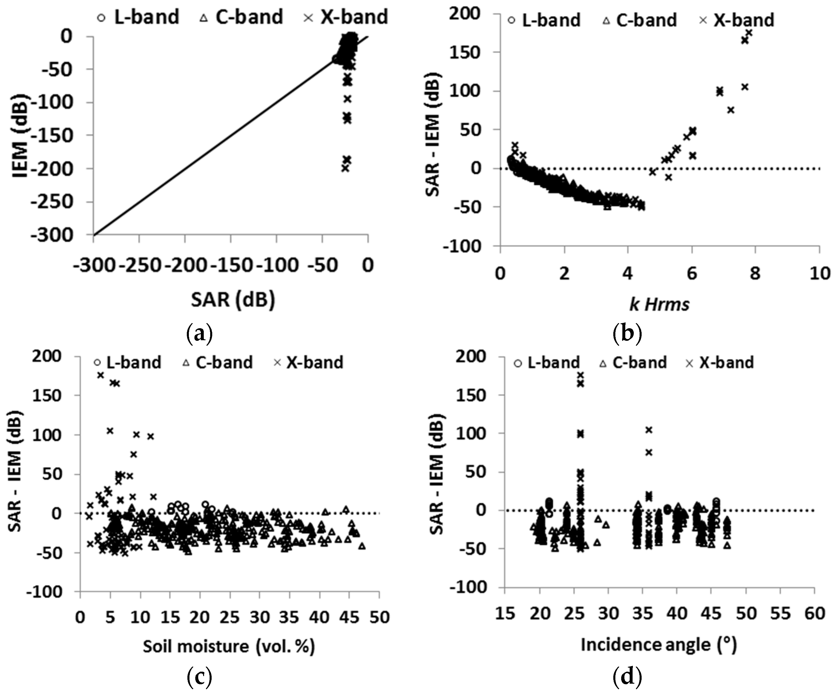
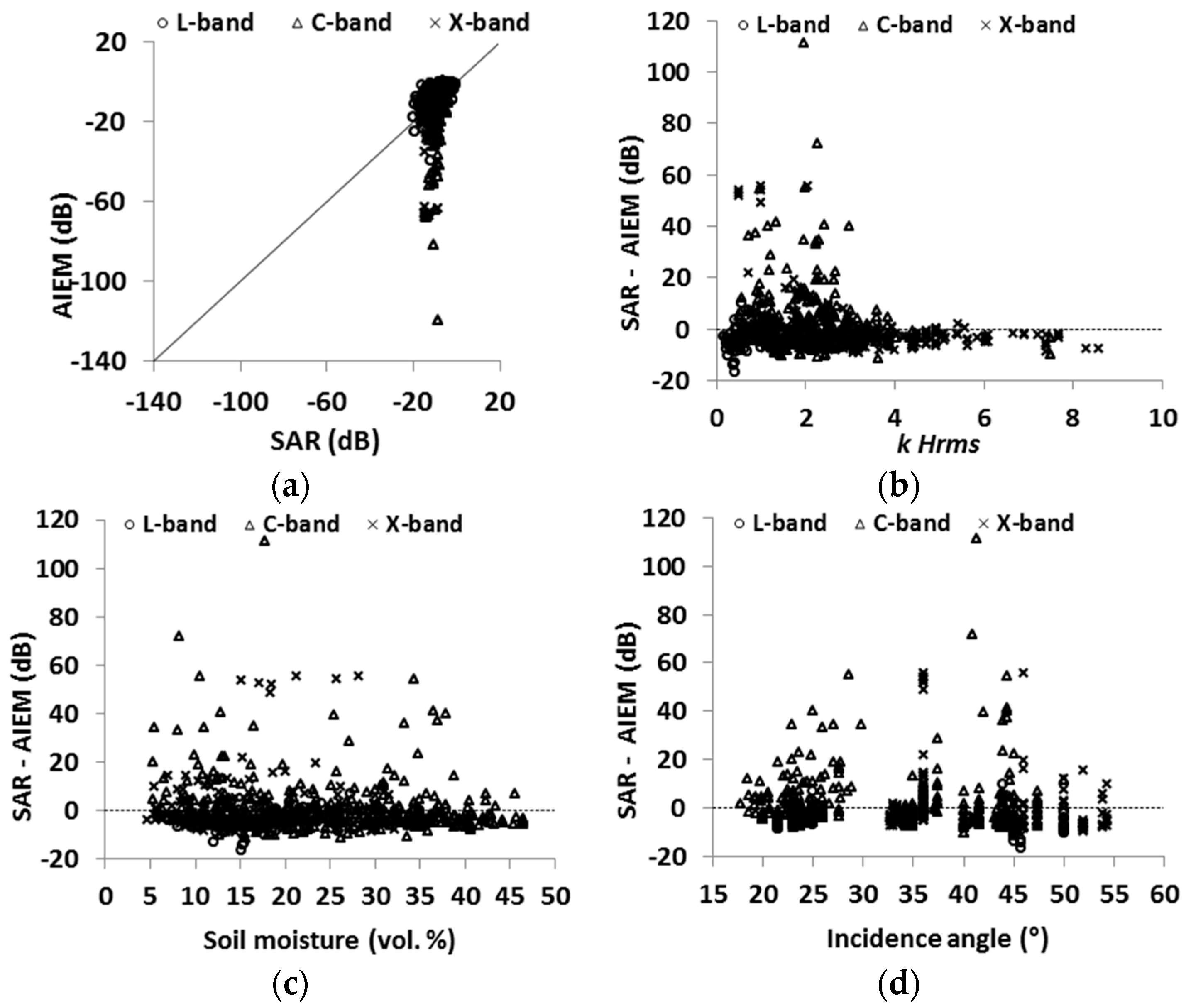
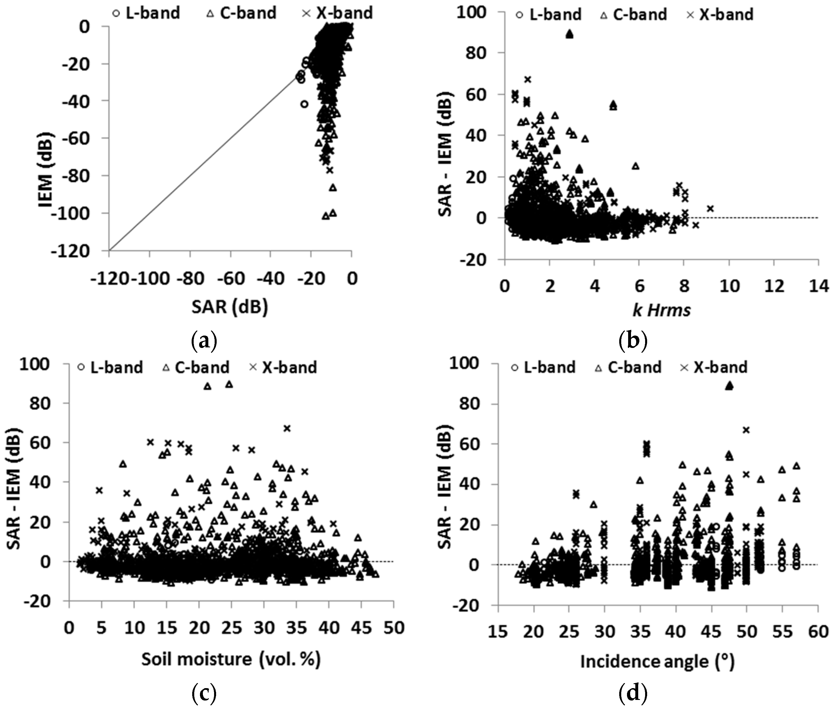
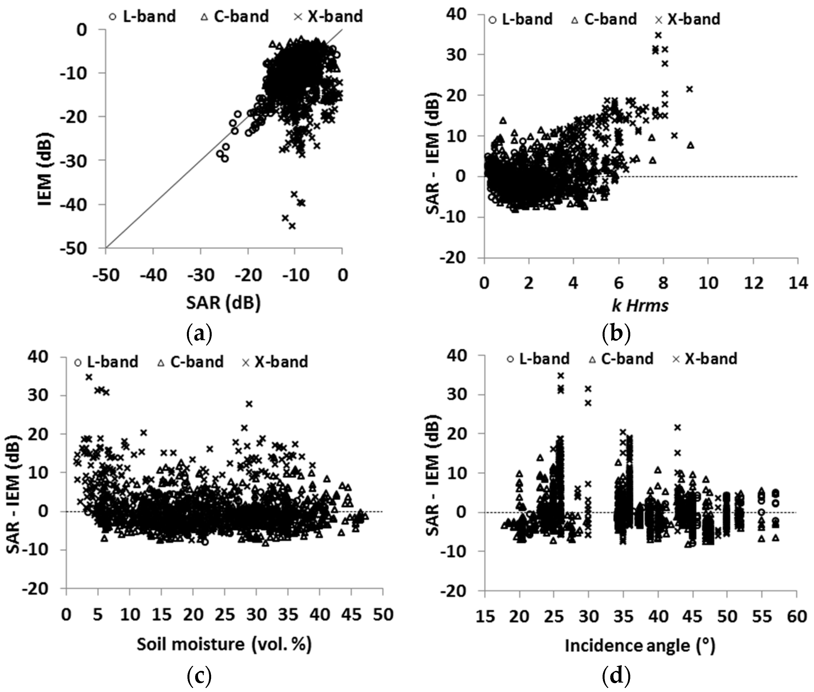
4.3. Evaluation of the IEM

The IEM was tested on our dataset using both a Gaussian correlation function (GCF) and an exponential correlation function (ECF). The evaluation of the IEM was carried out firstly using the entire dataset, later on for each radar wavelength (L-, C- and X-bands) and finally according to the validity domain of the IEM (Equation (10)).
Using all data, the IEM simulates the backscattering in HH polarization with an RMSE of 10.5 dB and 5.6 dB for GCF and ECF, respectively (Table 4). At VV polarization, the RMSE is 9.2 dB for GCF and 6.5 dB for ECF. At HV polarization, the RMSE is higher than 30.0 dB for both GCF and ECF. Some points show a large discrepancy between the real data and the IEM simulations performed using both ECF and GCF (Figure 6, Figure 7, Figure 8, Figure 9, Figure 10 and Figure 11). In case of the ECF (Figure 9, Figure 10 and Figure 11), these points are mainly outside the IEM validity domain (Equation (10)). In case of GCF (Figure 6, Figure 7 and Figure 8), the huge error is due to the high sensitivity of the IEM to roughness parameters (Hrms and L). Using the GCF, the IEM underestimates the backscattering coefficients for data with low Hrms values (kHrms < 3), high L values (L > 4 cm) and with high incidence angle (θ > 35°). Using the ECF, the sensitivity of backscattering to the roughness parameters is much lower (Figure 9, Figure 10 and Figure 11). Altese et al. [59], Zribi et al. [23,60], and Callens et al. [61] showed that in agricultural areas, the ECF usually provides better agreement to real data than the GCF.
The results obtained in L-band show that the IEM simulates the backscattering in HH pol. using both GCF and ECF with differences between real data and model simulations ranges between −0.9 dB and +0.6 dB, with an RMSE of 3.6 dB for GCF and 2.9 dB for ECF (Table 4). At VV polarization, the IEM overestimates the backscattering by about 2.5 dB and 1.3 dB for GCF and ECF, respectively (RMSE of 5.0 dB for GCF and 3.5 dB for ECF). At HV polarization, the IEM simulates the backscattering using GCF with RMSE of 14.5 dB using GCF, and lower RMSE (6.8 dB) using ECF.
According to the results observed in C-band, the IEM simulates the backscattering using GCF with RMSE of 11.2 dB and 8.6 dB for HH and VV polarizations, respectively (Table 4). The RMSE is lower with ECF than GCF about 4.1 dB for HH and 4.9 dB for VV polarizations. At HV polarization, the RMSE is higher than 25.0 dB using both GCF and ECF.
The results obtained in X-band show that the IEM simulates the backscattering with higher RMSE than L- and C-bands, the RMSE in HH pol. being about 10.6 dB for GCF and 8.3 dB for ECF. At VV polarization, the RMSE is 11.3 dB for GCF and 9.4 dB for ECF. At HV polarization, the IEM simulates the backscattering with high RMSE which is larger than 54.0 dB using both GCF and ECF.
The analysis of the error was also studied according to the validity domain of the IEM (Equation (10)). Inside the validity domain, the RMSE is larger than 11.5 dB for both HH and VV polarizations using GCF. Better results were obtained using ECF, where the IEM correctly simulates the backscattering at both HH and VV polarizations with differences between real and simulated data between −1.2 dB and −0.9 dB with RMSE of 3.2 dB at HH and 3.7 dB at VV polarizations, using data concerning the IEM validity domain. Outside the IEM validity domain, the IEM simulates the backscattering with RMSE of 6.7 dB for HH and 3.1 dB for VV using GCF; whereas RMSE is 7.8 dB for HH and 9.4 dB for VV polarization using ECF. At HV polarizations, model simulations show large differences from real data for both GCF and ECF for points inside or outside the validity domain of the IEM (in this case, RMSE is larger than 20 dB). Errors observed on IEM simulations were also studied as a function of the difference between Lopt and the measured correlation length (L). Results show that the IEM using GCF gives poor simulations mainly when the measured correlation length was over-estimated (L > Lopt). In this case, the IEM strongly under-estimates the SAR backscatter. In addition, the performance of the IEM was also analyzed using ECF according to the difference between Lopt and L. Results show the same performance of the IEM whatever the difference between Lopt and L.
As a conclusion, we could say that the IEM better simulates the backscattering in L-band than in C- and X-bands. Moreover, the results show a better fitting with real data using ECF instead than GCF, which agrees with the validity domain of the IEM.

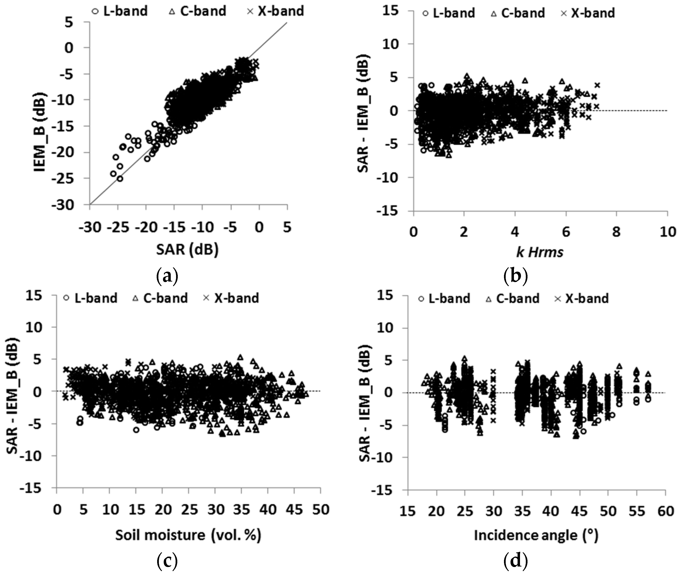
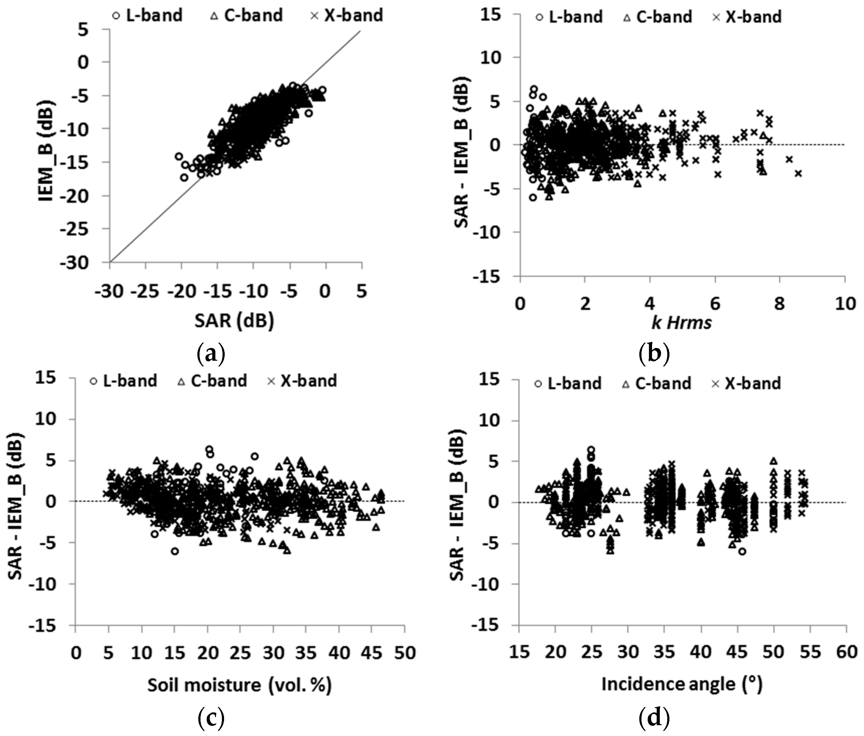
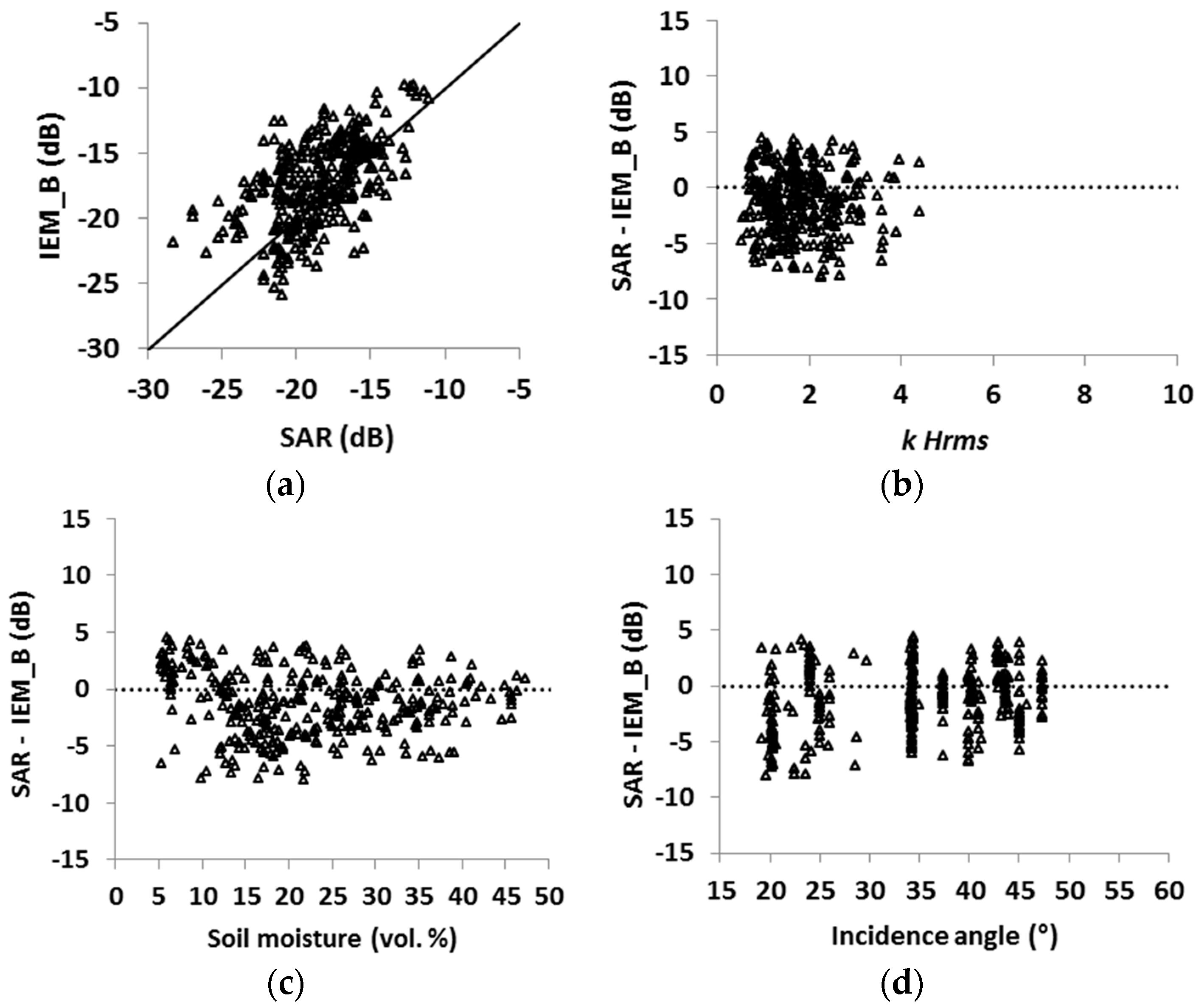
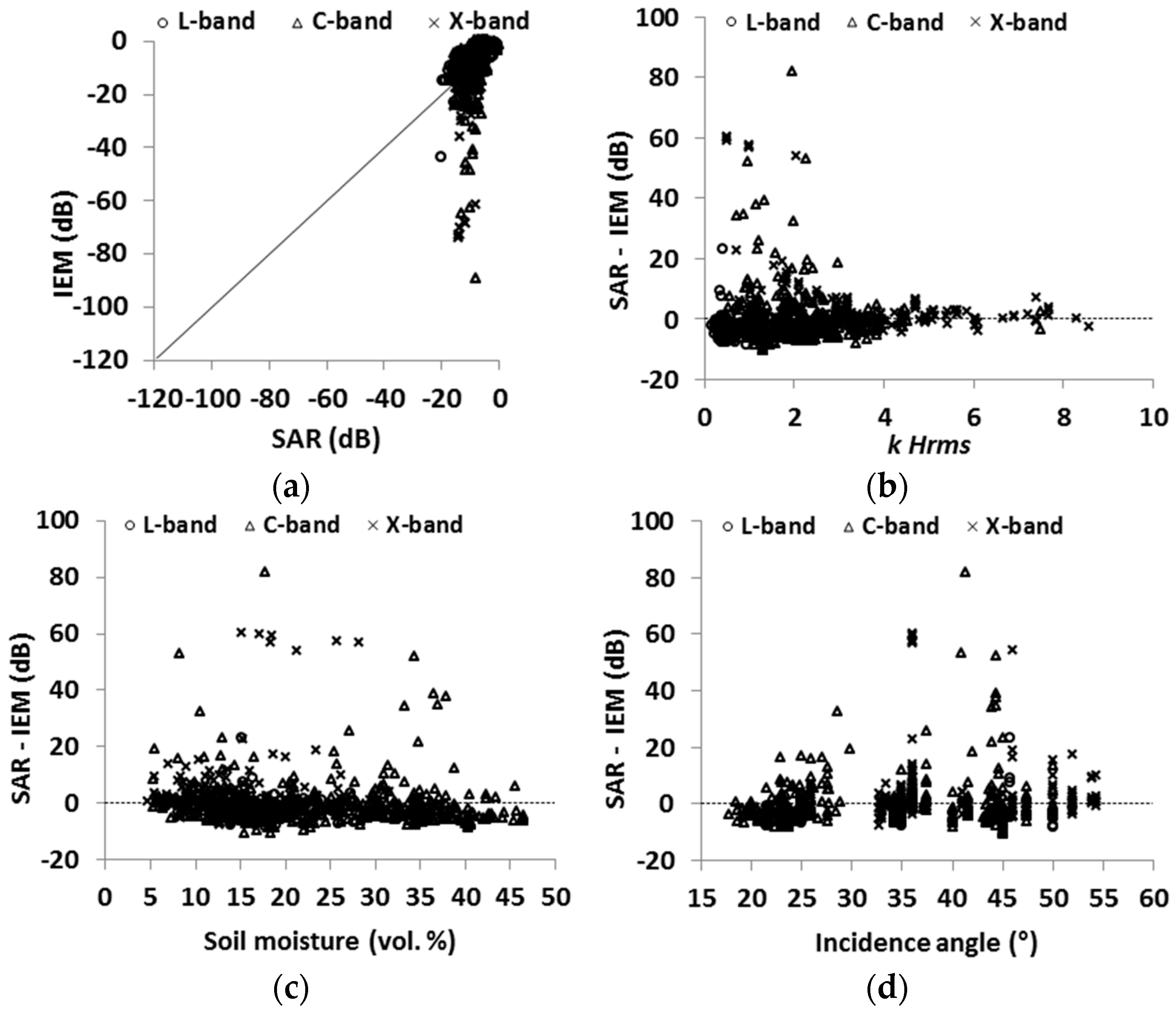
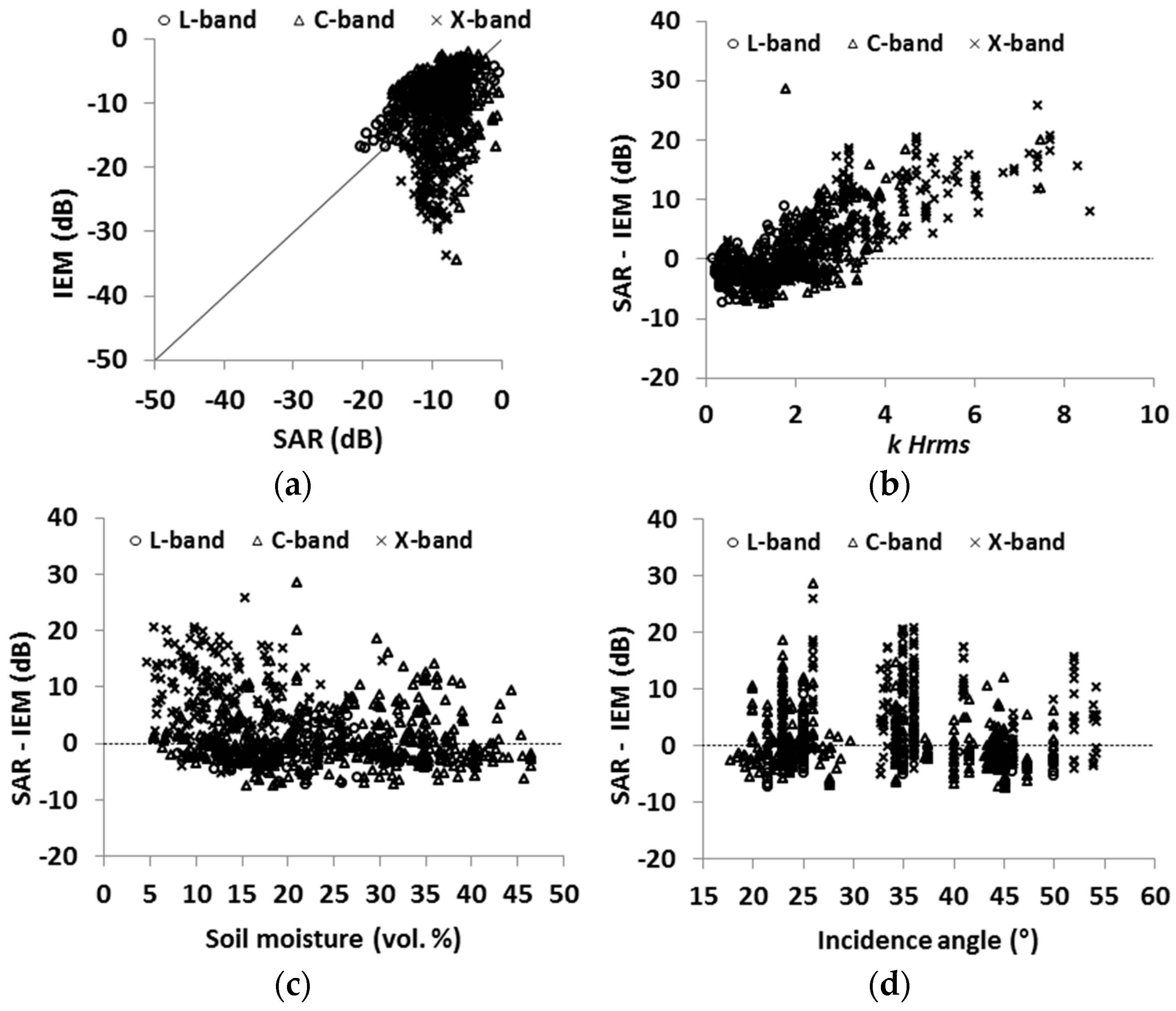
4.4. Evaluation of IEM Modified by Baghdadi (IEM_B)

The IEM_B was also tested on our dataset. This model version was run using GCF (Figure 12, Figure 13 and Figure 14). In comparison to the original IEM, results show that the RMSE was significantly lower. Using the entire dataset, the IEM_B correctly simulates the backscattering at both HH and VV polarizations showing low differences between real data and model simulations (−0.3 dB for HH and +0.1 dB for VV) with approximately similar RMSE of about 2.0 dB (Table 4). Moreover, the evaluation of the IEM_B was tested separately for each SAR band. Results show that the IEM_B correctly simulates the backscattering in comparison to the original model for all bands and in both HH and VV polarizations with a difference between real data and model simulations lower than 1.0 dB and with approximately similar RMSE between 1.8 and 2.3 dB (Table 4). At HV polarization, the IEM_B slightly over-estimates the backscattering by about 1.3 dB with RMSE of 3.1 dB, (the IEM_B was run only at C-band). Moreover, results show that the IEM_B simulations in both HH and VV pol., are slightly better in X- and C-bands than in L-band. The analysis of the difference between IEM_B simulations and SAR data versus the difference between Lopt and the measured correlation length (L) shows that IEM_B simulates well SAR data whatever the value of the difference between Lopt and L.

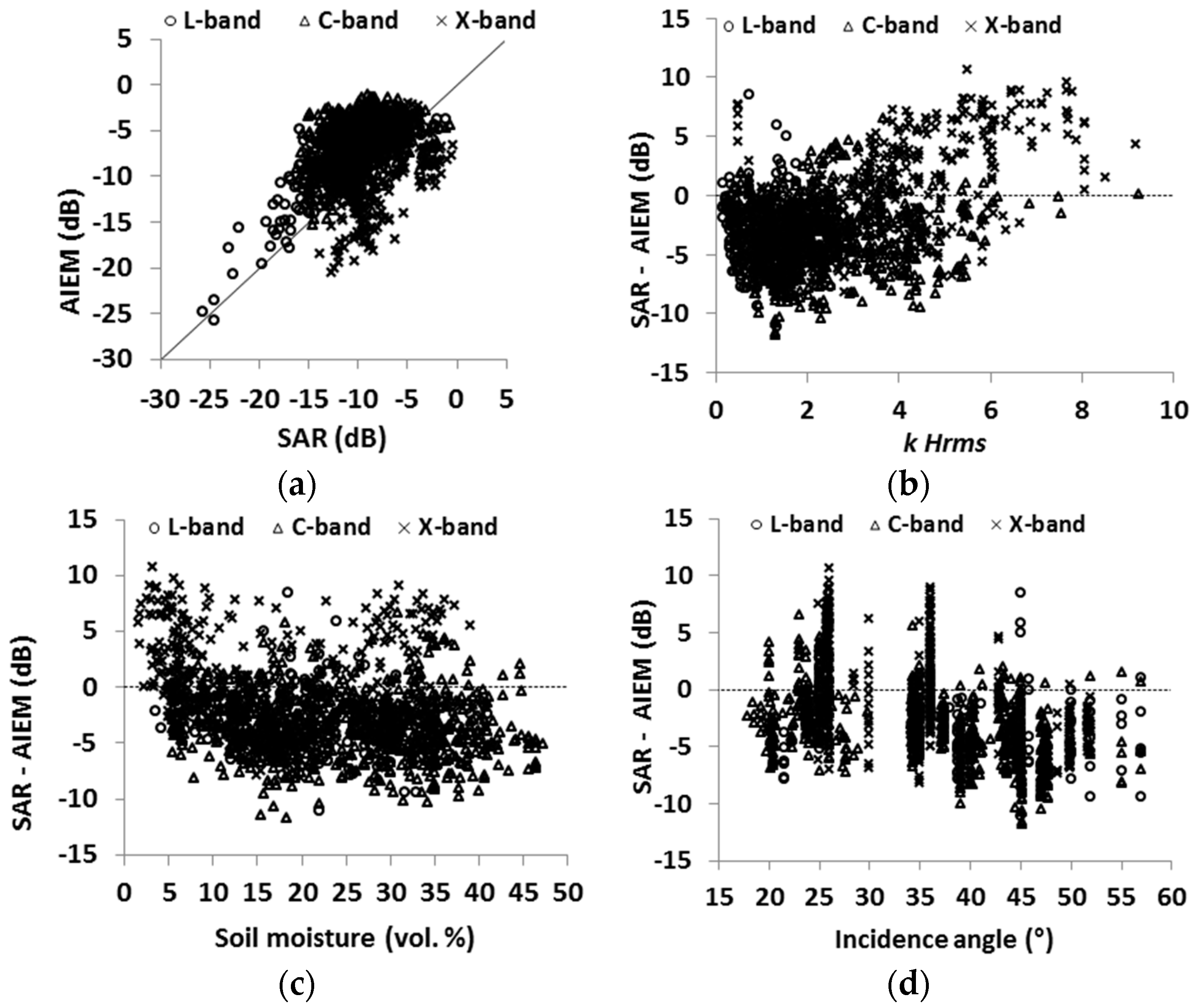
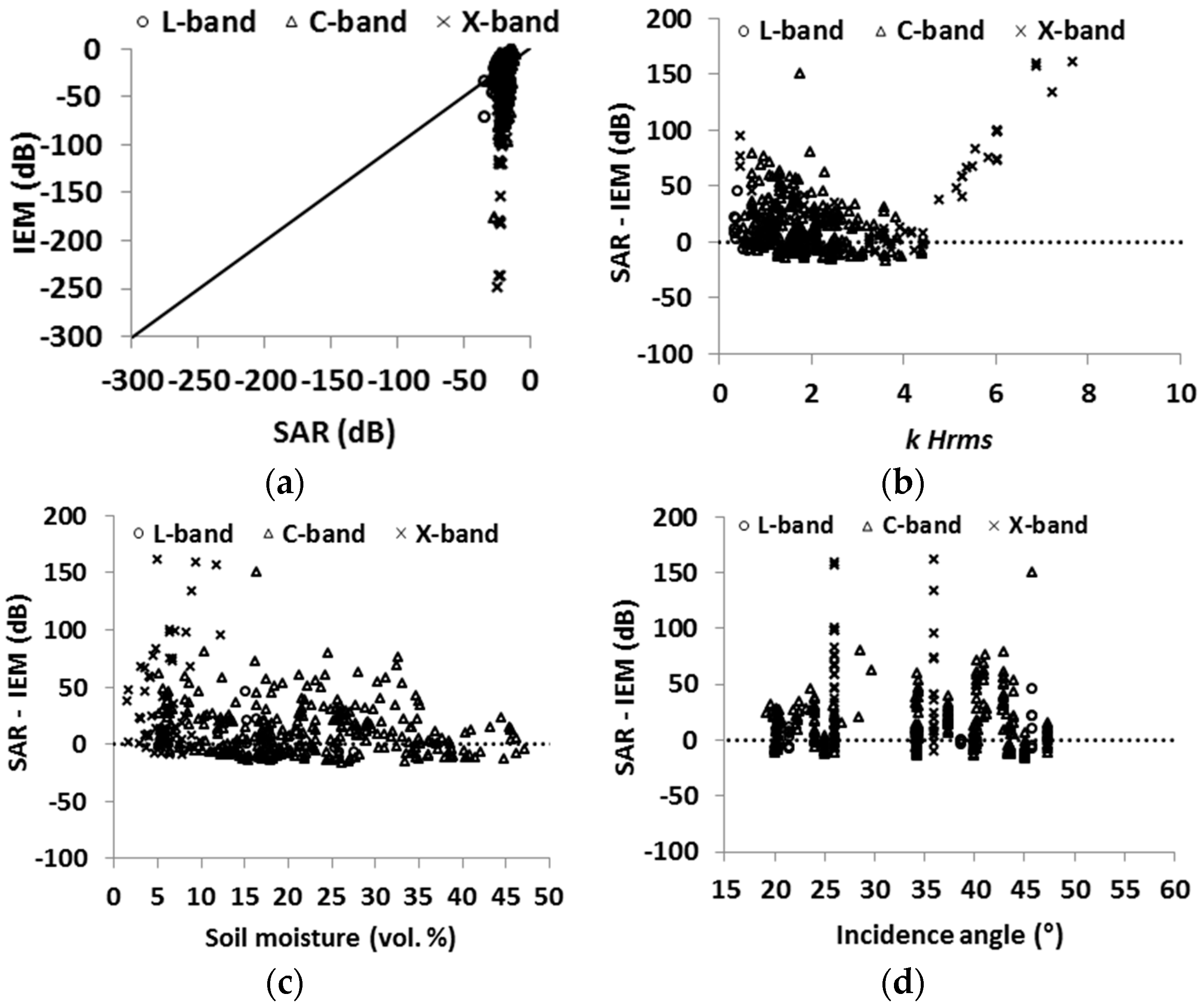
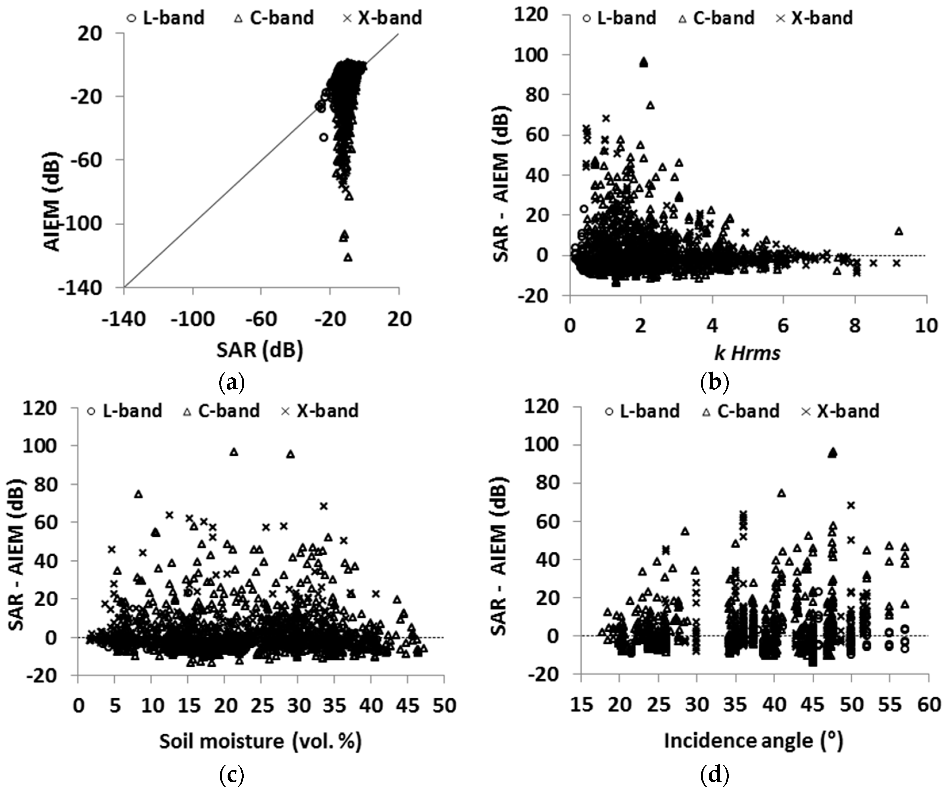
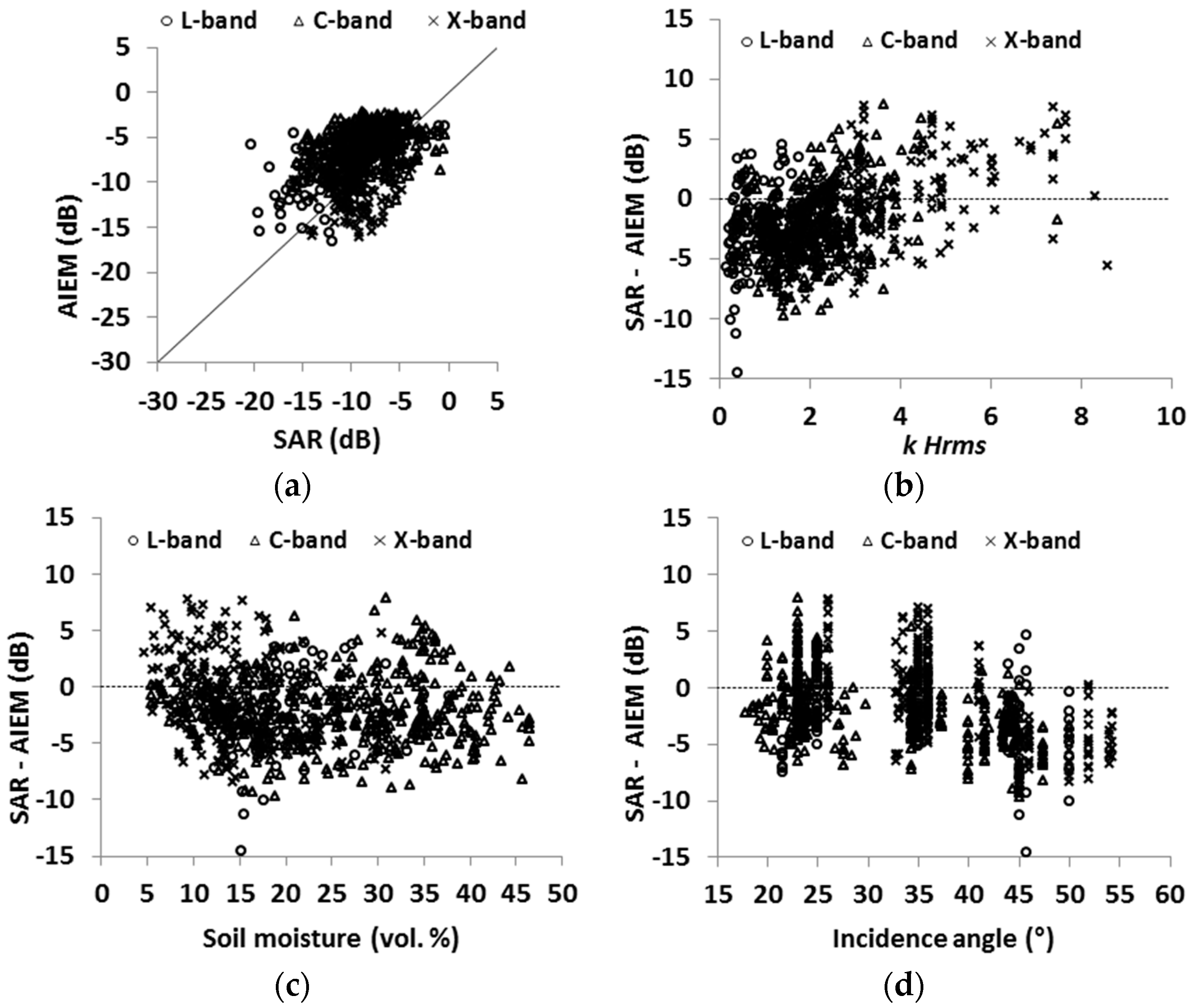
4.5. Evaluation of the Advanced Integral Equation Model (AIEM)

The AIEM was tested on our dataset at HH and VV polarizations using both GCF and ECF. For all data, the AIEM simulates the backscattering at HH and VV polarizations using GCF with RMSE larger than 10 dB (Table 4, Figure 15 and Figure 16). Moreover, results show better agreements of the AIEM with real data using ECF (Figure 17 and Figure 18). Indeed, the AIEM tends to overestimates the backscattering by about 2.3 dB at HH and 1.8 dB at VV (RMSE is 4.4 dB for HH and 3.8 dB for VV). Using the ECF, Figure 17 and Figure 18 show high overestimations of the backscattering for low values of surface roughness (kHrms < 4) and for incidence angles higher than 35°. Moreover, Figure 17 and Figure 18 show high underestimation of the radar signal (using ECF) in both HH and VV polarizations for points with high surface roughness (kHrms > 6), low mv-values (mv < 5 vol. %, and with low incidence angles (θ < 20°). Figure 15 and Figure 16 show that some points show high discrepancies between the real data and the AIEM simulations using GCF. Due to the high sensitivity to surface roughness of the AIEM using GCF, these points correspond mainly to surface with kHrms < 3, L > 4 cm and θ > 35°.
The performance of the AIEM was also evaluated for each SAR wavelength. Results show that in L-band the AIEM simulates the backscattering with RMSE of about 5.0 dB at both HH and VV polarizations using the GCF. In C and X-bands, the AIEM using GCF simulates the backscattering with RMSE higher than in L-band (RMSE > 11 dB). Moreover, AIEM better simulates better the backscattering in using GCF than ECF for all wavelength (RMSE about 4 dB).
In conclusions, the AIEM is able to better simulate better the backscattering than the original IEM only using the ECF with better results in X-band than in C- and L-bands.

5. Conclusions

Physical (IEM, IEM_B and AIEM) and semi-empirical (Oh and Dubois) backscattering models were tested using a wide dataset composed by large intervals of surface conditions (mv between 2 vol. % and 47 vol. %, Hrms between 0.2 cm and 9.6 cm and kHrms from 0.2 and 13.4), the dataset was acquired over bare soils in various agricultural study sites (France, Italy, Germany, Belgium, Luxembourg, Canada and Tunisia) characterized by large variety of climatological conditions and using SAR sensors in L-, C- and X-bands with incidence angle between 18° and 57°.
Results show that the IEM modified by Baghdadi (IEM_B used the empirical correlation length instead of measured correlation length) provides the most accurate SAR simulations (bias lower than 1.0 dB and RMSE lower than 2.0 dB) with slightly better performance in X-band (RMSE = 1.8 dB) than in L- and C-bands (RMSE between 1.9 and 2.3 dB). At HV polarization, the IEM_B was only run at C-band. Results show that the RMSE strongly decreases from values higher than 25.1 dB, using the original IEM, to 3.1 dB, using IEM_B. In contrast, high RMSE were found using both IEM and AIEM using Gaussian correlation function (RMSE higher than 9.2 dB) for both HH and VV polarizations because of the high sensitivity of the Gaussian correlation function to roughness parameters, mainly for kHrms < 3 and L > 4 cm. Moreover, results show better simulations of measured backscattering coefficients for both IEM and AIEM using exponential correlation function (RMSE > 5.6 dB for IEM and RMSE > 3.8 dB for AIEM) at HH and VV polarizations. At HV polarization, IEM results show very high errors (RMSE larger than 30.0 dB using both Gaussian correlation function and exponential correlation function). The AIEM better simulates the backscattering than the original IEM only using the exponential correlation function with slightly better results in X-band than in C- and L-bands. In contrast, the IEM simulates better the backscattering in L- band than C- and X-bands (Table 4).
Using the empirical models, all the Oh model versions show good agreements (RMSE < 3.0 dB) with measured backscattering with slightly better performance of the Oh 1992 version (bias less than 1.0 dB and RMSE less than 2.6 dB) at both HH and VV polarizations. The Oh model provides better results than Dubois model which simulates the backscattering in HH with RMSE of 4.0 dB, and slightly better simulations for VV with RMSE of 2.9 dB. At HV polarization, the Oh 2002 version correctly simulates the backscattering with difference between real and simulated data of about +0.7 dB and RMSE of 2.9 dB. The performance of the Oh 1992 version in HH and VV polarizations is better in C- and X-bands (bias between −1.2 and +0.4 dB with RMSE < 2.5 dB) than in L-band (bias > +2.0 with RMSE > 3.0 dB).
It should be mentioned that the use of different in situ sampling methods and SAR acquisition techniques may also contribute to the modelling errors. Indeed, the datasets comprises both airborne and space-borne acquisitions, which may cause scaling effects. In addition, in situ data have been collected using different techniques, both regarding soil moisture (gravimetric and TDR, sometimes at different sampling depths) and roughness (different profile length and sampling intervals, and post-processing methods).
This study evaluated the robustness of the most used backscattering models by means of statistical indices (Bias and RMSE). These statistical indices should guide in choosing the appropriate model for backscattering coefficients simulation. As it has been shown in the present study, the IEM modified by Baghdadi (IEM_B) was the most accurate model among the others. Thus, it is preferred to use the IEM_B in the inversion procedure of SAR backscattering coefficient in order to more accurately estimate soil moisture and roughness parameters.

Acknowledgments

Authors are grateful to the space agencies for kindly providing the AIRSAR, SIR-C, JERS-1, ERS-1/2, RADARSAT-1/2, ASAR, PALSAR-1, TerraSAR-X, COSMO-SkyMed, and ESAR data. This research is supported by IRSTEA (National Research Institute of Science and Technology for Environment and Agriculture), the French Space Study Center (CNES, TOSCA 2016), the French ANR (ANR AMETHYST project) and the Belgian Science Policy Office (Contract SR/00/302). Hans Lievens is a postdoctoral research of the Research Foundation Flanders (FWO).

Author Contributions

Mohammad Choker and Nicolas Baghdadi conceived and designed the experiments; Mohammad Choker performed the experiments; Mohammad Choker and Nicolas Baghdadi analyzed the data; Mehrez Zribi, Mohammad El Hajj, Simonetta Paloscia, Niko E. C. Verhoest, Hans Lievens, Francesco Mattia revised the manuscript; Mohammad Choker wrote the paper.

Conflicts of Interest

The authors declare no conflict of interest.

References

  1. Condrea, P.; Bostan, I. Environmental issues from an economic perspective. Environ. Eng. Manag. J. 2008, 7, 843–849. [Google Scholar]
  2. Costantini, E.A. Soil indicators to assess the effectiveness of restoration strategies in dryland ecosystems. Solid Earth 2016, 7, 397. [Google Scholar] [CrossRef] [Green Version]
  3. Lakshmi, V. Remote sensing of soil moisture. ISRN Soil Sci. 2013, 21, 336–344. [Google Scholar] [CrossRef]
  4. Aubert, M.; Baghdadi, N.; Zribi, M.; Douaoui, A.; Loumagne, C.; Baup, F.; El Hajj, M.; Garrigues, S. Analysis of TerraSAR-X data sensitivity to bare soil moisture, roughness, composition and soil crust. Remote Sens. Environ. 2011, 115, 1801–1810. [Google Scholar] [CrossRef] [Green Version]
  5. Hajnsek, I.; Jagdhuber, T.; Schon, H.; Papathanassiou, K.P. Potential of estimating soil moisture under vegetation cover by means of PolSAR. IEEE Trans. Geosci. Remote Sens. 2009, 47, 442–454. [Google Scholar] [CrossRef]
  6. Holah, N.; Baghdadi, N.; Zribi, M.; Bruand, A.; King, C. Potential of ASAR/ENVISAT for the characterization of soil surface parameters over bare agricultural fields. Remote Sens. Environ. 2005, 96, 78–86. [Google Scholar] [CrossRef] [Green Version]
  7. Paloscia, S.; Pampaloni, P.; Pettinato, S.; Santi, E. A comparison of algorithms for retrieving soil moisture from ENVISAT/ASAR images. IEEE Trans. Geosci. Remote Sens. 2008, 46, 3274–3284. [Google Scholar] [CrossRef]
  8. Oh, Y. Quantitative retrieval of soil moisture content and surface roughness from multipolarized radar observations of bare soil surfaces. IEEE Trans. Geosci. Remote Sens. 2004, 42, 596–601. [Google Scholar] [CrossRef]
  9. Oh, Y.; Sarabandi, K.; Ulaby, F.T. An empirical model and an inversion technique for radar scattering from bare soil surfaces. IEEE Trans. Geosci. Remote Sens. 1992, 30, 370–381. [Google Scholar] [CrossRef]
  10. Oh, Y.; Sarabandi, K.; Ulaby, F.T. An inversion algorithm for retrieving soil moisture and surface roughness from polarimetric radar observation. In Proceedings of the IEEE International Geoscience and Remote Sensing Symposium (IGARSS ’94)—Surface and Atmospheric Remote Sensing: Technologies, Data Analysis and Interpretation, Pasadena, CA, USA, 8–12 August 1994; Volume 3, pp. 1582–1584.
  11. Oh, Y.; Sarabandi, K.; Ulaby, F.T. Semi-empirical model of the ensemble-averaged differential Mueller matrix for microwave backscattering from bare soil surfaces. IEEE Trans. Geosci. Remote Sens. 2002, 40, 1348–1355. [Google Scholar] [CrossRef]
  12. Dubois, P.C.; Van Zyl, J.; Engman, T. Measuring soil moisture with imaging radars. IEEE Trans. Geosci. Remote Sens. 1995, 33, 915–926. [Google Scholar] [CrossRef]
  13. Fung, A.K.; Li, Z.; Chen, K.-S. Backscattering from a randomly rough dielectric surface. IEEE Trans. Geosci. Remote Sens. 1992, 30, 356–369. [Google Scholar] [CrossRef]
  14. Baghdadi, N.; King, C.; Chanzy, A.; Wigneron, J.P. An empirical calibration of the integral equation model based on SAR data, soil moisture and surface roughness measurement over bare soils. Int. J. Remote Sens. 2002, 23, 4325–4340. [Google Scholar] [CrossRef]
  15. Baghdadi, N.; Gherboudj, I.; Zribi, M.; Sahebi, M.; King, C.; Bonn, F. Semi-empirical calibration of the IEM backscattering model using radar images and moisture and roughness field measurements. Int. J. Remote Sens. 2004, 25, 3593–3623. [Google Scholar] [CrossRef]
  16. Baghdadi, N.; Holah, N.; Zribi, M. Calibration of the Integral Equation Model for SAR data in C-band and HH and VV polarizations. Int. J. Remote Sens. 2006, 27, 805–816. [Google Scholar] [CrossRef]
  17. Baghdadi, N.; Chaaya, J.A.; Zribi, M. Semiempirical calibration of the integral equation model for SAR data in C-band and cross polarization using radar images and field measurements. IEEE Geosci. Remote Sens. Lett. 2011, 8, 14–18. [Google Scholar] [CrossRef]
  18. Baghdadi, N.; Saba, E.; Aubert, M.; Zribi, M.; Baup, F. Evaluation of radar backscattering models IEM, Oh, and Dubois for SAR data in X-band over bare soils. IEEE Geosci. Remote Sens. Lett. 2011, 8, 1160–1164. [Google Scholar] [CrossRef]
  19. Baghdadi, N.; Zribi, M.; Paloscia, S.; Verhoest, N.E.; Lievens, H.; Baup, F.; Mattia, F. Semi-empirical calibration of the integral equation model for co-polarized L-band backscattering. Remote Sens. 2015, 7, 13626–13640. [Google Scholar] [CrossRef] [Green Version]
  20. Chen, K.-S.; Wu, T.-D.; Tsang, L.; Li, Q.; Shi, J.; Fung, A.K. Emission of rough surfaces calculated by the integral equation method with comparison to three-dimensional moment method simulations. IEEE Trans. Geosci. Remote Sens. 2003, 41, 90–101. [Google Scholar] [CrossRef]
  21. Baghdadi, N.; Zribi, M. Evaluation of radar backscatter models IEM, OH and Dubois using experimental observations. Int. J. Remote Sens. 2006, 27, 3831–3852. [Google Scholar] [CrossRef]
  22. Mattia, F.; Le Toan, T.; Souyris, J.-C.; De Carolis, C.; Floury, N.; Posa, F.; Pasquariello, N.G. The effect of surface roughness on multifrequency polarimetric SAR data. IEEE Trans. Geosci. Remote Sens. 1997, 35, 954–966. [Google Scholar] [CrossRef]
  23. Zribi, M.; Taconet, O.; Le Hégarat-Mascle, S.; Vidal-Madjar, D.; Emblanch, C.; Loumagne, C.; Normand, M. Backscattering behavior and simulation comparison over bare soils using SIR-C/X-SAR and ERASME 1994 data over Orgeval. Remote Sens. Environ. 1997, 59, 256–266. [Google Scholar] [CrossRef]
  24. Mattia, F.; Davidson, M.W.; Le Toan, T.; D’Haese, C.M.; Verhoest, N.E.; Gatti, A.M.; Borgeaud, M. A comparison between soil roughness statistics used in surface scattering models derived from mechanical and laser profilers. IEEE Trans. Geosci. Remote Sens. 2003, 41, 1659–1671. [Google Scholar] [CrossRef]
  25. Verhoest, N.E.; Lievens, H.; Wagner, W.; Álvarez-Mozos, J.; Moran, M.S.; Mattia, F. On the soil roughness parameterization problem in soil moisture retrieval of bare surfaces from synthetic aperture radar. Sensors 2008, 8, 4213–4248. [Google Scholar] [CrossRef] [PubMed]
  26. Ulaby, F.T.; Dubois, P.C.; Van Zyl, J. Radar mapping of surface soil moisture. J. Hydrol. 1996, 184, 57–84. [Google Scholar] [CrossRef]
  27. Baghdadi, N.; Paillou, P.; Grandjean, G.; Dubois, P.; Davidson, M. Relationship between profile length and roughness variables for natural surfaces. Int. J. Remote Sens. 2000, 21, 3375–3381. [Google Scholar] [CrossRef]
  28. Davidson, M.W.; Le Toan, T.; Mattia, F.; Satalino, G.; Manninen, T.; Borgeaud, M. On the characterization of agricultural soil roughness for radar remote sensing studies. IEEE Trans. Geosci. Remote Sens. 2000, 38, 630–640. [Google Scholar] [CrossRef]
  29. Le Toan, T.; Davidson, M.; Mattia, F.; Borderies, P.; Chenerie, I.; Manninen, T.; Borgeaud, M. Improved observation and modelling of bare soil surfaces for soil moisture retrieval. Earth Obs. Q. 1999, 62, 20–24. [Google Scholar]
  30. Lievens, H.; Verhoest, N.E.C.; Keyser, E.D.; Vernieuwe, H.; Matgen, P.; Alvarez-Mozos, J.; Baets, B.D. Effective roughness modelling as a tool for soil moisture retrieval from C-and L-band SAR. Hydrol. Earth Syst. Sci. 2011, 15, 151–162. [Google Scholar] [CrossRef] [Green Version]
  31. De Keyser, E.; Vernieuwe, H.; Lievens, H.; Alvarez-Mozos, J.; De Baets, B.; Verhoest, N.E. Assessment of SAR-retrieved soil moisture uncertainty induced by uncertainty on modeled soil surface roughness. Int. J. Appl. Earth Obs. Geoinf. 2012, 18, 176–182. [Google Scholar] [CrossRef]
  32. Verhoest, N.E.C.; De Baets, B.; Mattia, F.; Satalino, G.; Lucau, C.; Defourny, P. A possibilistic approach to soil moisture retrieval from ERS synthetic aperture radar backscattering under soil roughness uncertainty. Water Resour. Res. 2007, 43. [Google Scholar] [CrossRef]
  33. Lievens, H.; Verhoest, N.E. Spatial and temporal soil moisture estimation from RADARSAT-2 imagery over Flevoland, The Netherlands. J. Hydrol. 2012, 456, 44–56. [Google Scholar] [CrossRef]
  34. Rahman, M.M.; Moran, M.S.; Thoma, D.P.; Bryant, R.; Sano, E.E.; Holifield Collins, C.D.; Skirvin, S.; Kershner, C.; Orr, B.J. A derivation of roughness correlation length for parameterizing radar backscatter models. Int. J. Remote Sens. 2007, 28, 3995–4012. [Google Scholar] [CrossRef]
  35. Panciera, R.; Tanase, M.A.; Lowell, K.; Walker, J.P. Evaluation of IEM, Dubois, and Oh radar backscatter models using airborne L-band SAR. IEEE Trans. Geosci. Remote Sens. 2014, 52, 4966–4979. [Google Scholar] [CrossRef]
  36. Dong, L.; Baghdadi, N.; Ludwig, R. Validation of the AIEM through correlation length parameterization at field scale using radar imagery in a semi-arid environment. IEEE Geosci. Remote Sens. Lett. 2013, 10, 461–465. [Google Scholar] [CrossRef] [Green Version]
  37. McNairn, H.; Merzouki, A.; Pacheco, A. Estimating surface soil moisture using Radarsat-2. Int. Arch. Photogramm. Remote Sens. Spat. Inf. Sci. 2010, 38, 576–579. [Google Scholar]
  38. Baghdadi, N.; Dubois-Fernandez, P.; Dupuis, X.; Zribi, M. Sensitivity of main polarimetric parameters of multifrequency polarimetric SAR data to soil moisture and surface roughness over bare agricultural soils. IEEE Geosci. Remote Sens. Lett. 2013, 10, 731–735. [Google Scholar] [CrossRef] [Green Version]
  39. Baghdadi, N.; Zribi, M.; Loumagne, C.; Ansart, P.; Anguela, T.P. Analysis of TerraSAR-X data and their sensitivity to soil surface parameters over bare agricultural fields. Remote Sens. Environ. 2008, 112, 4370–4379. [Google Scholar] [CrossRef]
  40. Baghdadi, N.; Aubert, M.; Zribi, M. Use of TerraSAR-X data to retrieve soil moisture over bare soil agricultural fields. IEEE Geosci. Remote Sens. Lett. 2012, 9, 512–516. [Google Scholar] [CrossRef] [Green Version]
  41. Baghdadi, N.; King, C.; Bourguignon, A.; Remond, A. Potential of ERS and RADARSAT data for surface roughness monitoring over bare agricultural fields: Application to catchments in Northern France. Int. J. Remote Sens. 2002, 23, 3427–3442. [Google Scholar] [CrossRef]
  42. Baghdadi, N.; Holah, N.; Zribi, M. Soil moisture estimation using multi-incidence and multi-polarization ASAR data. Int. J. Remote Sens. 2006, 27, 1907–1920. [Google Scholar] [CrossRef]
  43. Baghdadi, N.; Saba, E.; Aubert, M.; Zribi, M.; Baup, F. Comparison between backscattered TerraSAR signals and simulations from the radar backscattering models IEM, Oh, and Dubois. IEEE Geosci. Remote Sens. Lett. 2011, 6, 1160–1164. [Google Scholar] [CrossRef]
  44. Baghdadi, N.; Aubert, M.; Cerdan, O.; Franchistéguy, L.; Viel, C.; Eric, M.; Zribi, M.; Desprats, J.F. Operational mapping of soil moisture using synthetic aperture radar data: Application to the Touch basin (France). Sensors 2007, 7, 2458–2483. [Google Scholar] [CrossRef]
  45. Zribi, M.; Gorrab, A.; Baghdadi, N.; Lili-Chabaane, Z.; Mougenot, B. Influence of radar frequency on the relationship between bare surface soil moisture vertical profile and radar backscatter. IEEE Geosci. Remote Sens. Lett. 2014, 11, 848–852. [Google Scholar] [CrossRef] [Green Version]
  46. Gorrab, A.; Zribi, M.; Baghdadi, N.; Mougenot, B.; Fanise, P.; Chabaane, Z.L. Retrieval of both soil moisture and texture using TerraSAR-X images. Remote Sens. 2015, 7, 10098–10116. [Google Scholar] [CrossRef] [Green Version]
  47. Aubert, M.; Baghdadi, N.N.; Zribi, M.; Ose, K.; El Hajj, M.; Vaudour, E.; Gonzalez-Sosa, E. Toward an operational bare soil moisture mapping using TerraSAR-X data acquired over agricultural areas. IEEE J. Sel. Top. Appl. Earth Obs. Remote Sens. 2013, 6, 900–916. [Google Scholar] [CrossRef] [Green Version]
  48. Baronti, S.; Del Frate, F.; Ferrazzoli, P.; Paloscia, S.; Pampaloni, P.; Schiavon, G. SAR polarimetric features of agricultural areas. Int. J. Remote Sens. 1995, 16, 2639–2656. [Google Scholar] [CrossRef]
  49. Macelloni, G.; Paloscia, S.; Pampaloni, P.; Sigismondi, S.; De Matthaeis, P.; Ferrazzoli, P.; Schiavon, G.; Solimini, D. The SIR-C/X-SAR experiment on Montespertoli: Sensitivity to hydrological parameters. Int. J. Remote Sens. 1999, 20, 2597–2612. [Google Scholar] [CrossRef]
  50. Paloscia, S.; Macelloni, G.; Pampaloni, P.; Sigismondi, S. The potential of C-and L-band SAR in estimating vegetation biomass: The ERS-1 and JERS-1 experiments. IEEE Trans. Geosci. Remote Sens. 1999, 37, 2107–2110. [Google Scholar] [CrossRef]
  51. Oh, Y.; Kay, Y.C. Condition for precise measurement of soil surface roughness. IEEE Trans. Geosci. Remote Sens. 1998, 36, 691–695. [Google Scholar]
  52. Hallikainen, M.T.; Ulaby, F.T.; Dobson, M.C.; El-Rayes, M.A.; Wu, L.-K. Microwave dielectric behavior of wet soil-part 1: Empirical models and experimental observations. IEEE Trans. Geosci. Remote Sens. 1985, GE-23, 25–34. [Google Scholar] [CrossRef]
  53. Rakotoarivony, L.; Taconet, O.; Vidal-Madjar, D.; Bellemain, P.; Benallegue, M. Radar backscattering over agricultural bare soils. J. Electromagn. Waves Appl. 1996, 10, 187–209. [Google Scholar] [CrossRef]
  54. Remond, A. Image SAR: Potentialités D’extraction d’un Paramètre Physique du Ruissellement, la Rugosité (Modélisation et Expérimentation). Ph.D. Thesis, Université de Bourgogne, Dijon, France, 1997. [Google Scholar]
  55. Rakotoarivony, L. Validation de Modèles de Diffusion Electromagnétique: Comparaison Entre Simulations et Mesures Radar Héliporté sur des Surfaces Agricoles de sol nu. Ph.D. Thesis, Université de Caen, Caen, France, 1995. [Google Scholar]
  56. Boisvert, J.B.; Gwyn, Q.H.J.; Chanzy, A.; Major, D.J.; Brisco, B.; Brown, R.J. Effect of surface soil moisture gradients on modelling radar backscattering from bare fields. Int. J. Remote Sens. 1997, 18, 153–170. [Google Scholar] [CrossRef]
  57. Fung, A.K. Microwave Scattering and Emission Models and Their Applications; Artech House, Incorporated: Norwood, UK, 1994. [Google Scholar]
  58. Wu, T.-D.; Chen, K.-S.; Shi, J.; Fung, A.K. A transition model for the reflection coefficient in surface scattering. IEEE Trans. Geosci. Remote Sens. 2001, 39, 2040–2050. [Google Scholar]
  59. Altese, E.; Bolognani, O.; Mancini, M.; Troch, P.A. Retrieving soil moisture over bare soil from ERS 1 synthetic aperture radar data: Sensitivity analysis based on a theoretical surface scattering model and field data. Water Resour. Res. 1996, 32, 653–661. [Google Scholar] [CrossRef]
  60. Zribi, M.; Baghdadi, N.; Holah, N.; Fafin, O. New methodology for soil surface moisture estimation and its application to ENVISAT-ASAR multi-incidence data inversion. Remote Sens. Environ. 2005, 96, 485–496. [Google Scholar] [CrossRef]
  61. Callens, M.; Verhoest, N.E.; Davidson, M.W. Parameterization of tillage-induced single-scale soil roughness from 4-m profiles. IEEE Trans. Geosci. Remote Sens. 2006, 44, 878–888. [Google Scholar] [CrossRef]
Figure 1. Comparison between backscattering coefficient values obtained from SAR images and those estimated from the Dubois model at HH polarization. (a) Dubois model simulations vs. SAR data; (b) difference between SAR signal and the Dubois model vs. soil roughness (kHrms); (c) difference between SAR signal and the Dubois model vs. soil moisture (mv); (d) difference between SAR signal and Dubois model vs. incidence angle.
Water 09 00038 g001
Figure 2. Comparison between backscattering coefficient values obtained from SAR images and those estimated using the Dubois model at VV polarization. (a) Dubois model simulations vs. SAR data; (b) difference between SAR signal and Dubois model vs. soil roughness (kHrms); (c) difference between SAR signal and the Dubois model vs. soil moisture (mv); (d) difference between SAR signal and the Dubois model vs. incidence angle.
Water 09 00038 g002aWater 09 00038 g002b
Figure 3. Comparison between backscattering coefficients derived from SAR images and those estimated from the Oh 1992 model at HH polarization, (a) Oh model simulations vs. SAR data; (b) difference between SAR signal and Oh model results vs. soil roughness (kHrms); (c) difference between SAR signal and Oh model results vs. soil moisture (mv); (d) difference between SAR signal and Oh model results vs. incidence angle.
Water 09 00038 g003aWater 09 00038 g003b
Figure 4. Comparison between backscattering coefficients derived from SAR images and those estimated from the Oh 1992 model at VV polarization, (a) Oh simulations vs. SAR data; (b) difference between SAR signal and the Oh model vs. soil roughness (kHrms); (c) difference between SAR signal and Oh model results vs. soil moisture (mv); (d) difference between SAR signal and Oh model results vs. incidence angle.
Water 09 00038 g004
Figure 5. Comparison between backscattering coefficients derived from SAR images and those estimated from the Oh 2002 model at HV polarization, (a) Oh simulations vs. SAR data; (b) difference between SAR signal and Oh model results vs. soil roughness (kHrms); (c) difference between SAR signal and Oh model results vs. soil moisture (mv); (d) difference between SAR signal and Oh model results vs. incidence angle.
Water 09 00038 g005
Figure 6. Comparison between backscattering coefficients derived from SAR images and those estimated from IEM at HH polarization using GCF. (a) IEM simulations vs. SAR data; (b) difference between SAR signal and IEM vs. soil roughness (kHrms); (c) difference between SAR signal and IEM vs. soil moisture (mv); (d) difference between SAR signal and IEM vs. incidence angle.
Water 09 00038 g006
Figure 7. Comparison between backscattering coefficients derived from SAR images and those estimated from IEM at VV polarization using GCF. (a) IEM simulations vs. SAR data; (b) difference between SAR signal and IEM vs. soil roughness (kHrms); (c) difference between SAR signal and IEM vs. soil moisture (mv); (d) difference between SAR signal and IEM vs. incidence angle.
Water 09 00038 g007
Figure 8. Comparison between backscattering coefficients derived from SAR images and those estimated from IEM at HV polarization using GCF. (a) IEM simulations vs. SAR data; (b) difference between SAR signal and IEM vs. soil roughness (kHrms); (c) difference between SAR signal and IEM vs. soil moisture (mv); (d) difference between SAR signal and IEM vs. incidence angle.
Water 09 00038 g008
Figure 9. Comparison between backscattering coefficients derived from SAR images and those estimated from IEM at HH polarization using ECF. (a) IEM simulations vs. SAR data; (b) difference between SAR signal and IEM vs. soil roughness (kHrms); (c) difference between SAR signal and IEM vs. soil moisture (mv); (d) difference between SAR signal and IEM vs. incidence angle.
Water 09 00038 g009
Figure 10. Comparison between backscattering coefficients derived from SAR images and those estimated from IEM at VV polarization using ECF. (a) IEM simulations vs. SAR data; (b) difference between SAR signal and IEM vs. soil roughness (kHrms); (c) difference between SAR signal and IEM vs. soil moisture (mv); (d) difference between SAR signal and IEM vs. incidence angle.
Water 09 00038 g010
Figure 11. Comparison between backscattering coefficients derived from SAR images and those estimated from IEM at HV polarization using ECF. (a) IEM simulations vs. SAR data; (b) difference between SAR signal and IEM vs. soil roughness (kHrms); (c) difference between SAR signal and IEM vs. soil moisture (mv); (d) difference between SAR signal and IEM vs. incidence angle.
Water 09 00038 g011
Figure 12. Comparison between backscattering coefficients derived from SAR images and those estimated from IEM_B at HH polarization using GCF. (a) IEM_B simulations vs. SAR data; (b) difference between SAR signal and IEM_B vs. soil roughness (kHrms); (c) difference between SAR signal and IEM_B vs. soil moisture (mv); (d) difference between SAR signal and IEM_B vs. incidence angle.
Water 09 00038 g012
Figure 13. Comparison between backscattering coefficients derived from SAR images and those estimated from IEM_B at VV polarization using GCF. (a) IEM_B simulations vs. SAR data; (b) difference between SAR signal and IEM_B vs. soil roughness (kHrms); (c) difference between SAR signal and IEM_B vs. soil moisture (mv); (d) difference between SAR signal and IEM_B vs. incidence angle.
Water 09 00038 g013
Figure 14. Comparison between backscattering coefficients derived from SAR images and those estimated from IEM_B in C-band at HV polarization using GCF. (a) IEM_B simulations vs. SAR data; (b) difference between SAR signal and IEM_B vs. soil roughness (kHrms); (c) difference between SAR signal and IEM_B vs. soil moisture (mv); (d) difference between SAR signal and IEM_B vs. incidence angle.
Water 09 00038 g014
Figure 15. Comparison between backscattering coefficients derived from SAR images and those estimated from AIEM at HH polarization using GCF. (a) AIEM simulations vs. SAR data; (b) difference between SAR signal and AIEM vs. soil roughness (kHrms); (c) difference between SAR signal and AIEM vs. soil moisture (mv); (d) difference between SAR signal and AIEM vs. incidence angle.
Water 09 00038 g015
Figure 16. Comparison between backscattering coefficients derived from SAR images and those estimated from AIEM at VV polarization using GCF. (a) AIEM simulations vs. SAR data; (b) difference between SAR signal and AIEM vs. soil roughness (kHrms); (c) difference between SAR signal and AIEM vs. soil moisture (mv); (d) difference between SAR signal and AIEM vs. incidence angle.
Water 09 00038 g016
Figure 17. Comparison between backscattering coefficients derived from SAR images and those estimated from AIEM at HH polarization using ECF. (a) AIEM simulations vs. SAR data; (b) difference between SAR signal and AIEM vs. soil roughness (kHrms); (c) difference between SAR signal and AIEM vs. soil moisture (mv); (d) difference between SAR signal and AIEM vs. incidence angle.
Water 09 00038 g017
Figure 18. Comparison between radar backscattering coefficients calculated from SAR images and those estimated from AIEM for VV polarization using ECF. (a) AIEM simulations vs. SAR data; (b) difference between SAR signal and AIEM vs. soil roughness (kHrms); (c) difference between SAR signal and AIEM vs. soil moisture (mv); (d) difference between SAR signal and AIEM vs. incidence angle.
Water 09 00038 g018
Table 1. Description of the dataset used in this study. “Fr”: France, “It”: Italy, “Ge”: Germany, “Be”: Belgium, “Lu”: Luxembourg, “Ca”: Canada, “Tu”: Tunisia.
SiteSAR SensorSpatial ResolutionFreqYearNumber of Data
Orgeval (Fr) [23]SIR-C30 m × 30 mL1994HH: 1262 measurements
66 in L-band
766 in C-band
430 in X-band
VV: 790 measurements
159 in L-band
411 in C-band
220 in X-band
HV: 390 measurements
13 in L-band
313 in C-band
64 in X-band
Orgeval (Fr) [23,38,39]SIR-C, ERS, ASAR30 m × 30 mC1994; 1995; 2008; 2009; 2010
Orgeval (Fr) [39]PALSAR-130 m × 30 mL2009
Orgeval (Fr) [40]TerraSAR-X1 m × 1 mX2008, 2009, 2010
Pays de Caux (Fr) [15,41]ERS; RADARSAT30 m × 30 mC1998; 1999
Villamblain (Fr) [6,16,42]
Villamblain (Fr) [39,43]
ASAR
TerraSAR-X
30 m × 30 mC
X
2003; 2004; 2006
2008; 2009
Thau (Fr) [44]RADARSAT
TerraSAR-X
30 m × 30 m
1 m × 1 m
C
X
2010; 2011 2010
Touch (Fr) [6,44]ERS-2; ASAR30 m × 30 mC2004; 2006; 2007
Mauzac (Fr) [43]TerraSAR-X1 m × 1 mX2009
Garons (Fr) [43]TerraSAR-X1 m × 1 mX2009
Kairouan (Tu) [45]
Kairouan (Tu) [43,45,46]
ASAR
TerraSAR-X
30 m × 30 mC
X
2012
2010; 2012; 2013; 2014
Yzerons (Fr) [47]TerraSAR-X1 m × 1 mX2009
Versailles (Fr) [43]TerraSAR-X1 m × 1 mX2010
Seysses (Fr) [43]TerraSAR-X1 m × 1 mX2010
Chateauguay (Ca) [15]RADARSAT30 m × 30 mC1999
Brochet (Ca) [15]RADARSAT30 m × 30 mC1999
Alpilles (Fr) [15]ERS; RADARSAT30 m × 30 mC1996; 1997
Sardaigne (It) [36]ASAR; RADARSAT30 m × 30 mC2008; 2009
Matera (It) [22]SIR-C30 m × 30 mL1994
Alzette (Lu) [30,34]PALSAR-130 m × 30 mL2008
Dijle (Be) [30]PALSAR-130 m × 30 mL2008; 2009
Zwalm (Be) [30]PALSAR-130 m × 30 mL2007
Demmin (Ge) [30]ESAR2 m × 2 mL2006
Montespertoli (It) [35,48]
Montespertoli (It) [49]
Montespertoli (It) [50]
AIRSAR
SIR-C
JERS-1
30 m × 30 mL
L; C
L
1991
1994
1994
Table 2. Comparison between the Dubois model output and real data using the entire dataset, and by separating two intervals of kHrms, soil moisture (mv) and incidence angle (θ). Bias = real data − simulations.
ModelStatisticsAll DataL-BandC-BandX-BandkHrms < 2.5kHrms > 2.5mv < 20 vol.%mv > 20 vol. %θ < 30°θ > 30°
Dubois for HH pol.Bias (dB)−1.0−1.0−1.1−0.9+0.4−2.9−2.6+0.3−4.2+0.3
RMSE (dB)4.03.04.14.13.64.64.63.45.53.2
Dubois for VV pol.Bias (dB)+0.7−0.2+0.4+1.8+1.2−0.2+0.5+1.0−0.6+1.5
RMSE (dB)2.92.52.83.13.02.52.83.02.92.9
Table 3. Comparison between real data and Oh models for all data and different ranges of kHrms and soil moisture (mv). Bias = real data − simulations.
ModelPol.StatisticsAll DataL-BandC-BandX-BandkHrms < 2.0kHrms > 2.0mv < 29.1 vol. %mv > 29.1 vol. %
Oh et al. (1992) [9]HHBias (dB)+0.4+2.5+0.10.0+1.3−0.5−0.3+1.9
RMSE (dB)2.63.72.42.52.92.32.33.1
VVBias (dB)+0.1+2.1+0.4−1.2+1.0−0.7−0.4+1.5
RMSE (dB)2.43.42.32.12.72.02.32.7
Oh et al. (1994) [10]HHBias (dB)−0.9+1.3−1.2−1.2−0.05−1.7−1.6+0.5
RMSE (dB)2.82.82.72.82.62.92.92.5
VVBias (dB)−1.3+0.7−1.3−2.1−0.5−2.1−1.7−0.4
RMSE (dB)2.62.62.62.72.42.92.82.2
Oh et al. (2002) [11]HHBias (dB)−0.3+2.1−0.9−1.0+0.3−0.9−0.7+0.4
RMSE (dB)2.73.22.72.82.72.62.72.5
HVBias (dB)+0.7+1.5+1.0−0.9+1.8−0.7+0.5+0.8
RMSE (dB)2.93.12.73.83.22.53.02.6
VVBias (dB)−0.6+1.8−1.2+0.4−0.2−1.0−0.7−0.5
RMSE (dB)2.52.92.72.02.52.62.62.5
Oh (2004) [8]HHBias (dB)−0.5+2.1−1.0−0.60.6+1.5−0.9+0.4
RMSE (dB)2.63.32.72.32.62.62.72.6
VVBias (dB)−1.1+1.4−1.5−1.4−0.2−2.0−1.3−0.8
RMSE (dB)2.62.82.82.12.42.82.62.6
Table 4. Comparison between real data and IEM versions (original model, IEM_B and AIEM) using both GCF and ECF. (1) all data; (2) for different SAR wavelength; (3) according to the validity domain of IEM. Bias = real data − model simulations.
ModelPol.StatisticsAll DataL-BandC-BandX-BandInside the Validity DomainOutside the Validity Domain
IEM using GCFHHBias (dB)+0.8−0.9+0.7+1.5+2.6−1.8
RMSE (dB)10.53.611.210.612.46.7
HVBias (dB)+17.2+5.2+11.8+46.3+18.0+14.1
RMSE (dB)38.414.526.774.028.550.1
VVBias (dB)+0.4−2.5+0.7+3.5+1.2−0.9
RMSE (dB)9.25.08.611.311.53.1
IEM using ECFHHBias (dB)+0.8+0.6−1.0+4.2−1.2+3.8
RMSE (dB)5.62.94.18.33.27.8
HVBias (dB)−15.8+1.2−19.90.0−15.8−17.1
RMSE (dB)31.46.825.154.420.144.3
VVBias (dB)+2.2−1.3+0.5+6.7−0.9+7.1
RMSE (dB)6.53.54.99.43.79.4
IEM_B with Lopt using GCFHHBias (dB)−0.3−0.1−0.6+0.3
RMSE (dB)2.02.32.11.8
HVBias (dB) −1.3
RMSE (dB)3.1
VVBias (dB)+0.1+0.20+0.3
RMSE (dB)1.92.31.91.8
AIEM using GCFHHBias (dB)+2.3−3.2+2.9+3.1
RMSE (dB)12.25.413.411.7
VVBias (dB)0.0−4.1+0.5+0.5
RMSE (dB)10.85.911.411.0
AIEM using ECFHHBias (dB)−2.3−3.0−3.6+0.2
RMSE (dB)4.44.44.64.2
VVBias (dB)−1.8−2.4−2.3-0.7
RMSE (dB)3.84.43.83.7

