
Effects of Model Spatial Resolution on Ecohydrologic Predictions and Their Sensitivity to Inter-Annual Climate Variability

Abstract
:1. Introduction
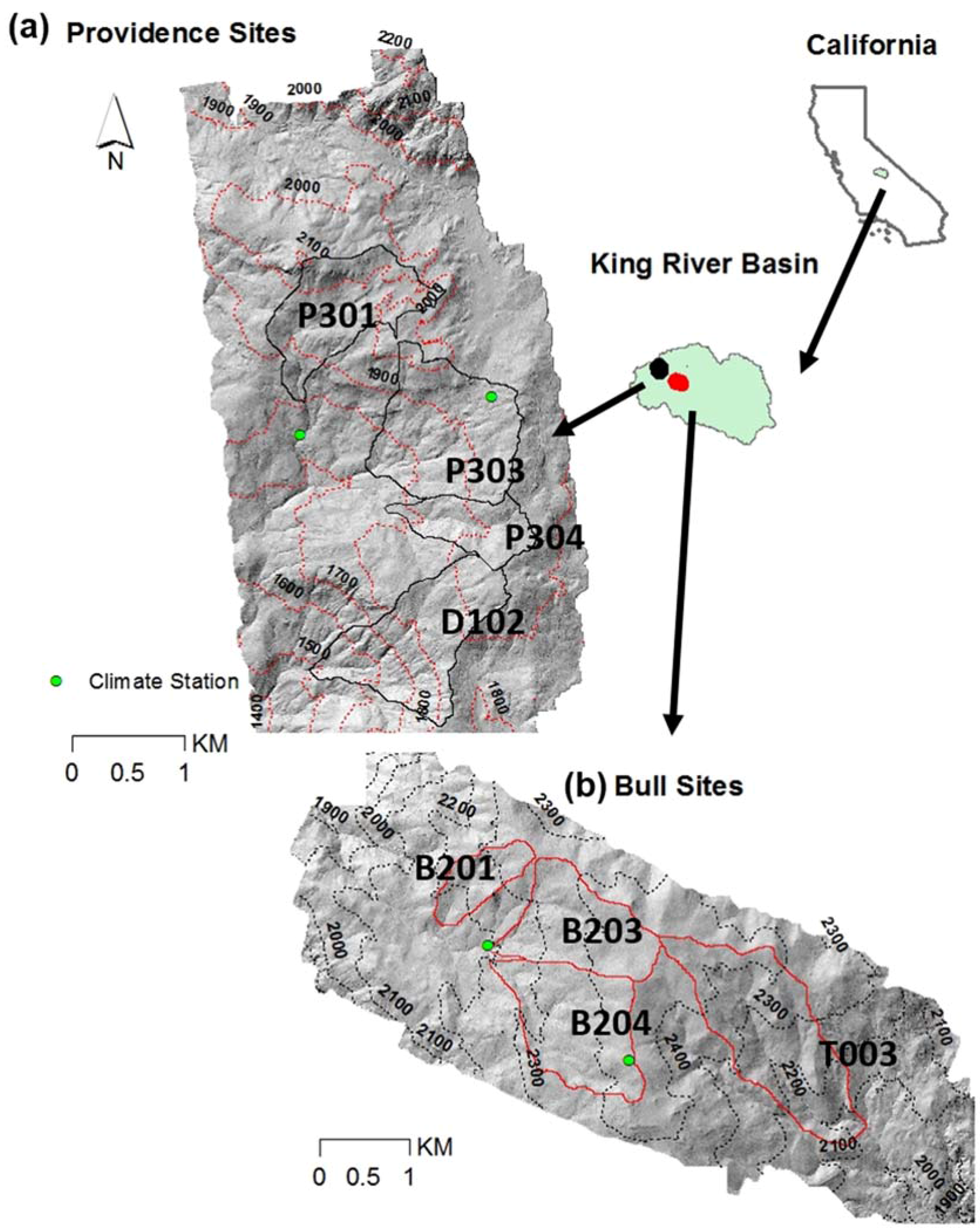
2. Research Sites
2.1. Providence Sites
2.2. Bull Sites
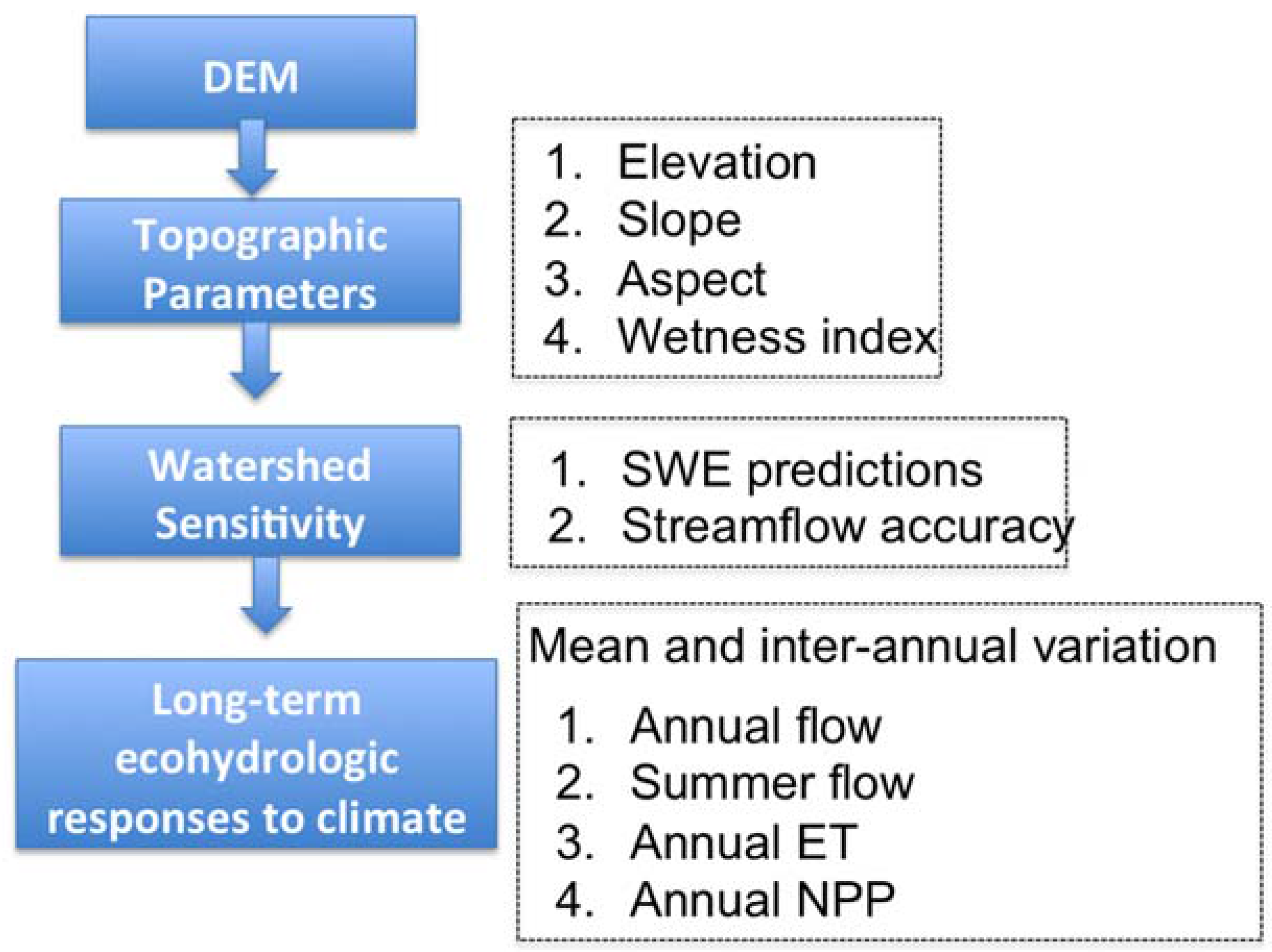
3. Methodology
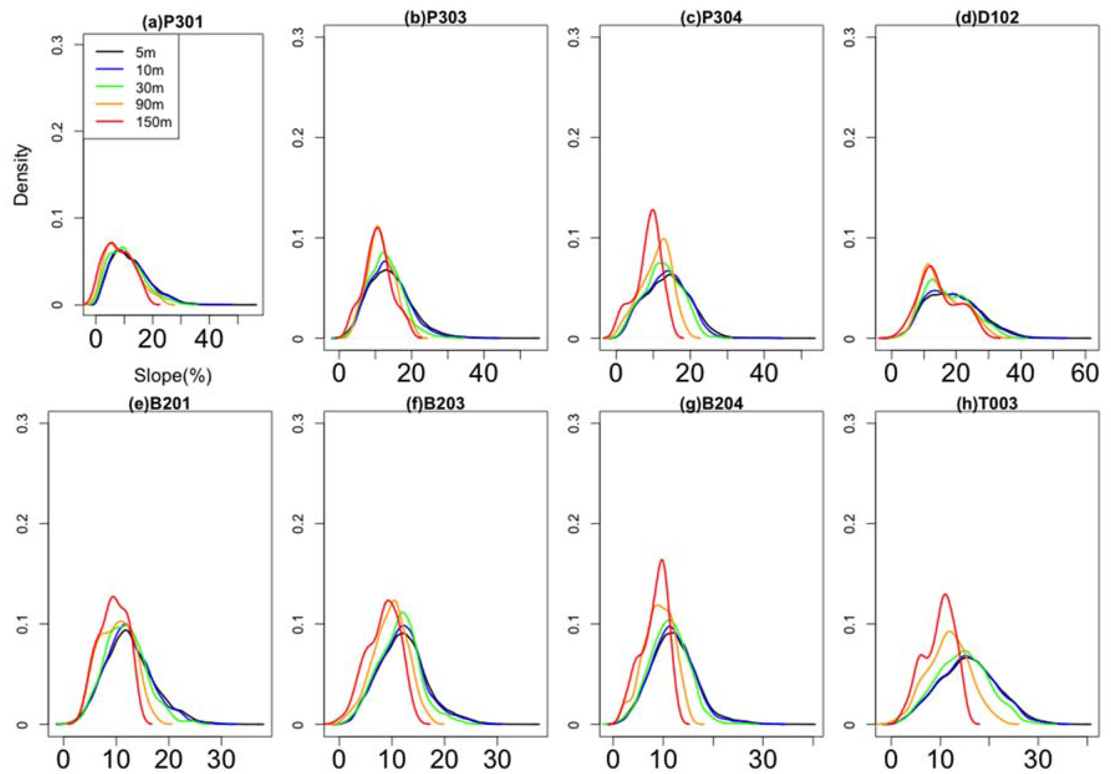
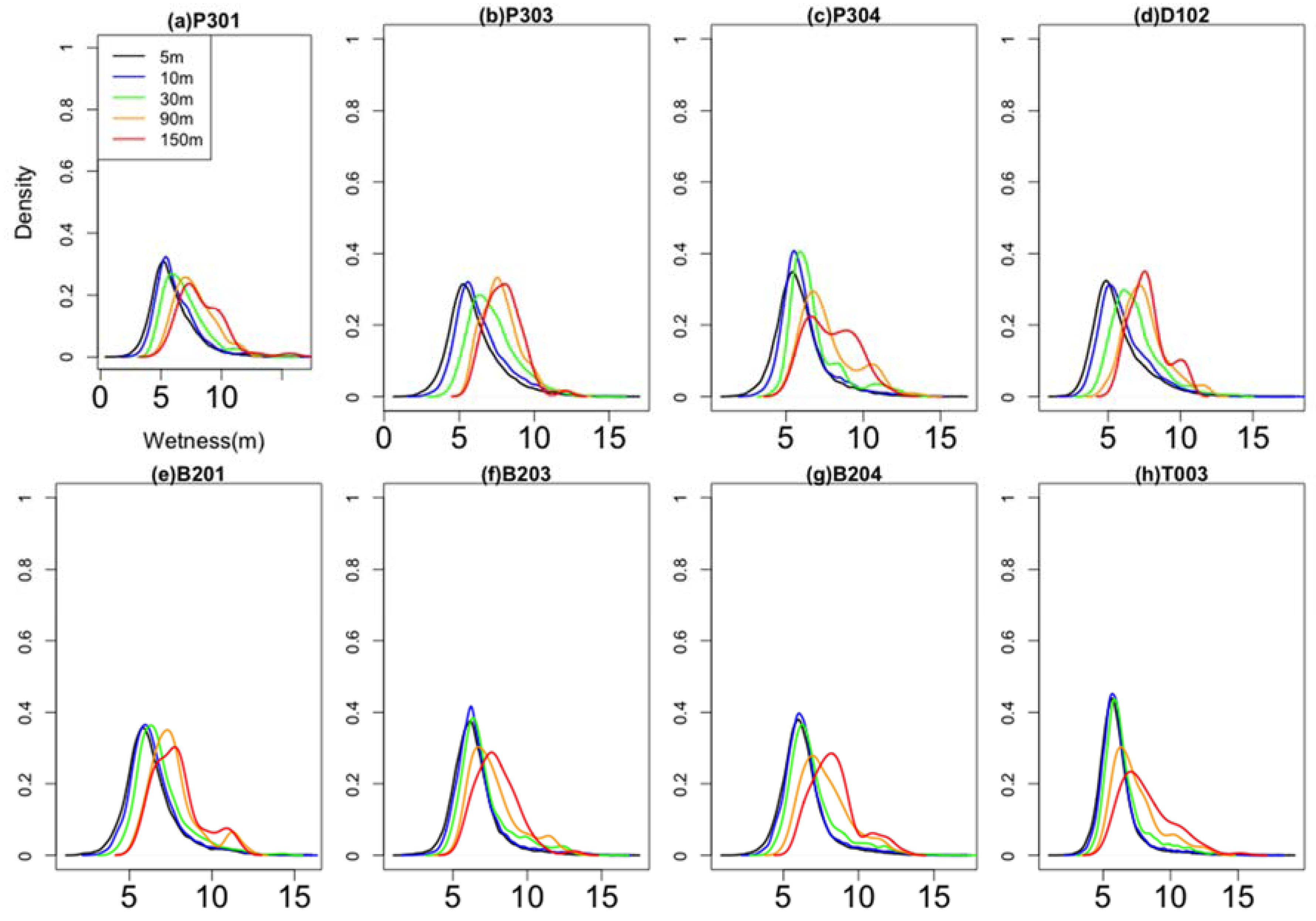
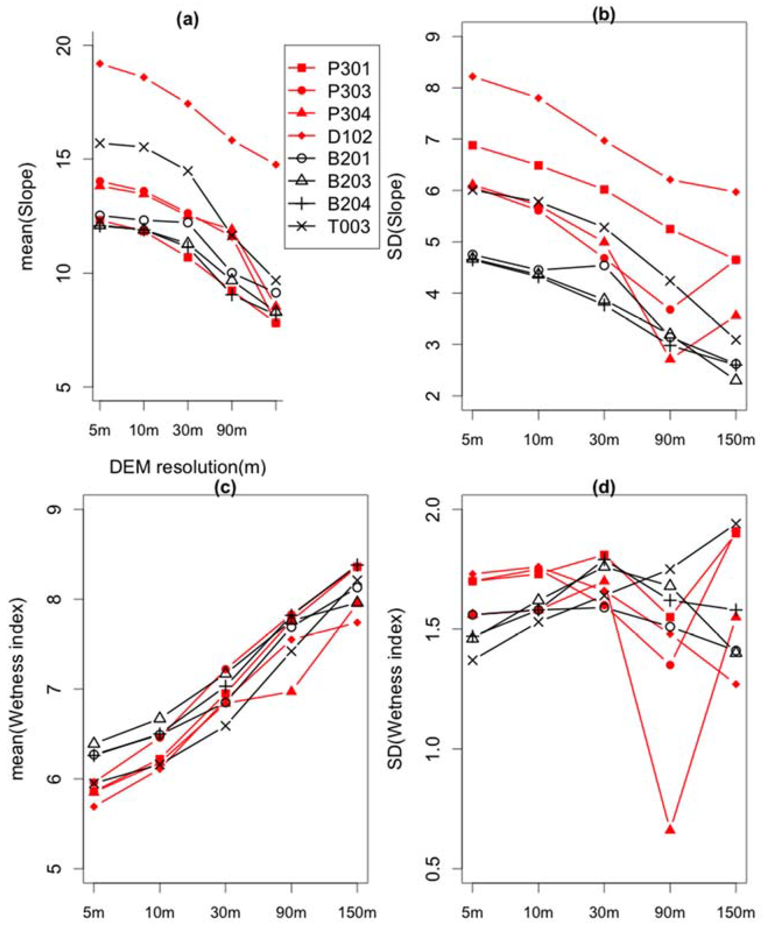
3.1. Effect of DEM Resolution on Topographic Parameters
3.2. Model Description
3.3. Model Calibration
3.4. Effect of DEM Resolution on Model Accuracy and Long-Term Ecohydrologic Responses to Climate
4. Results
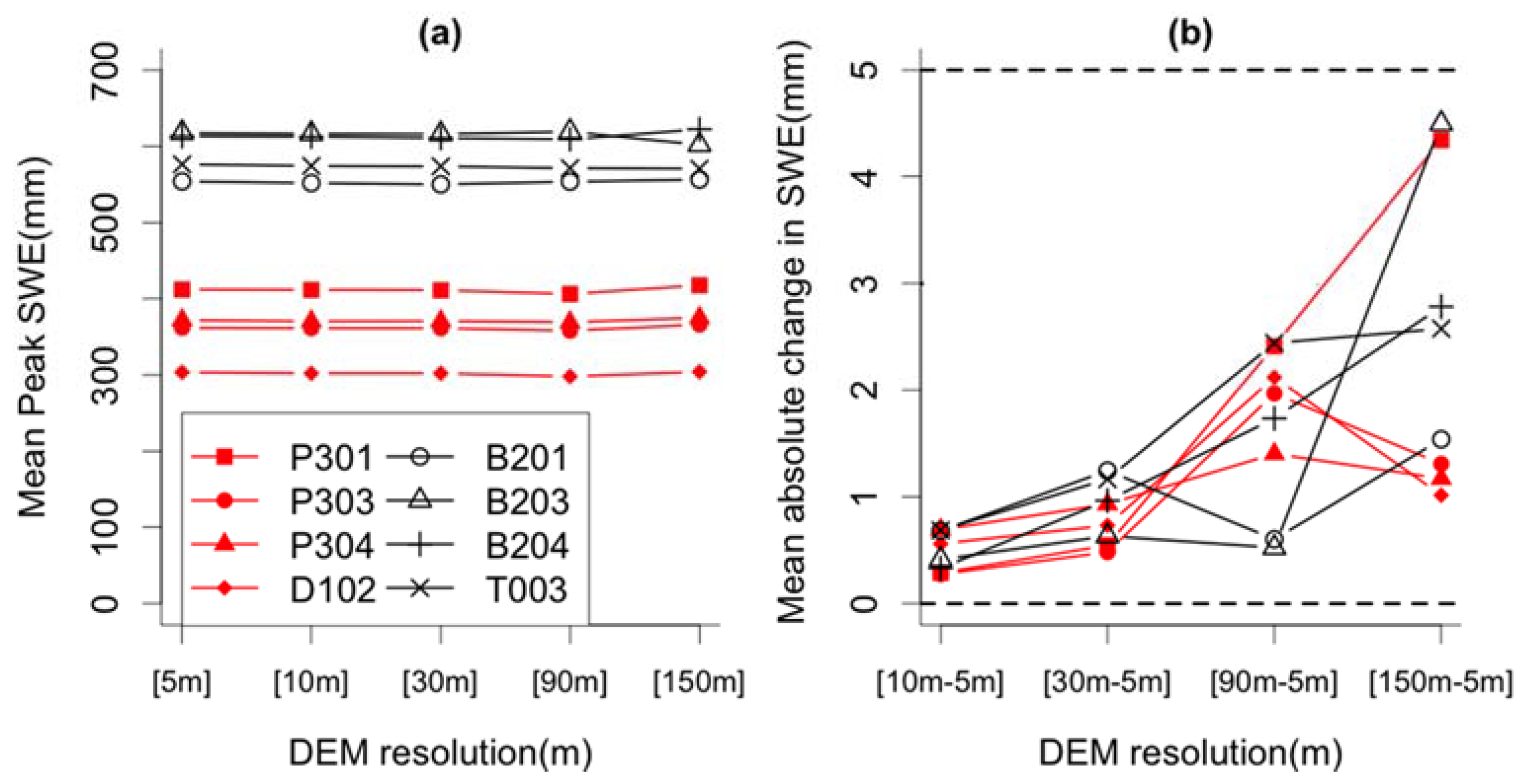
4.1. Effect of DEM Resolution on Snow Predictions
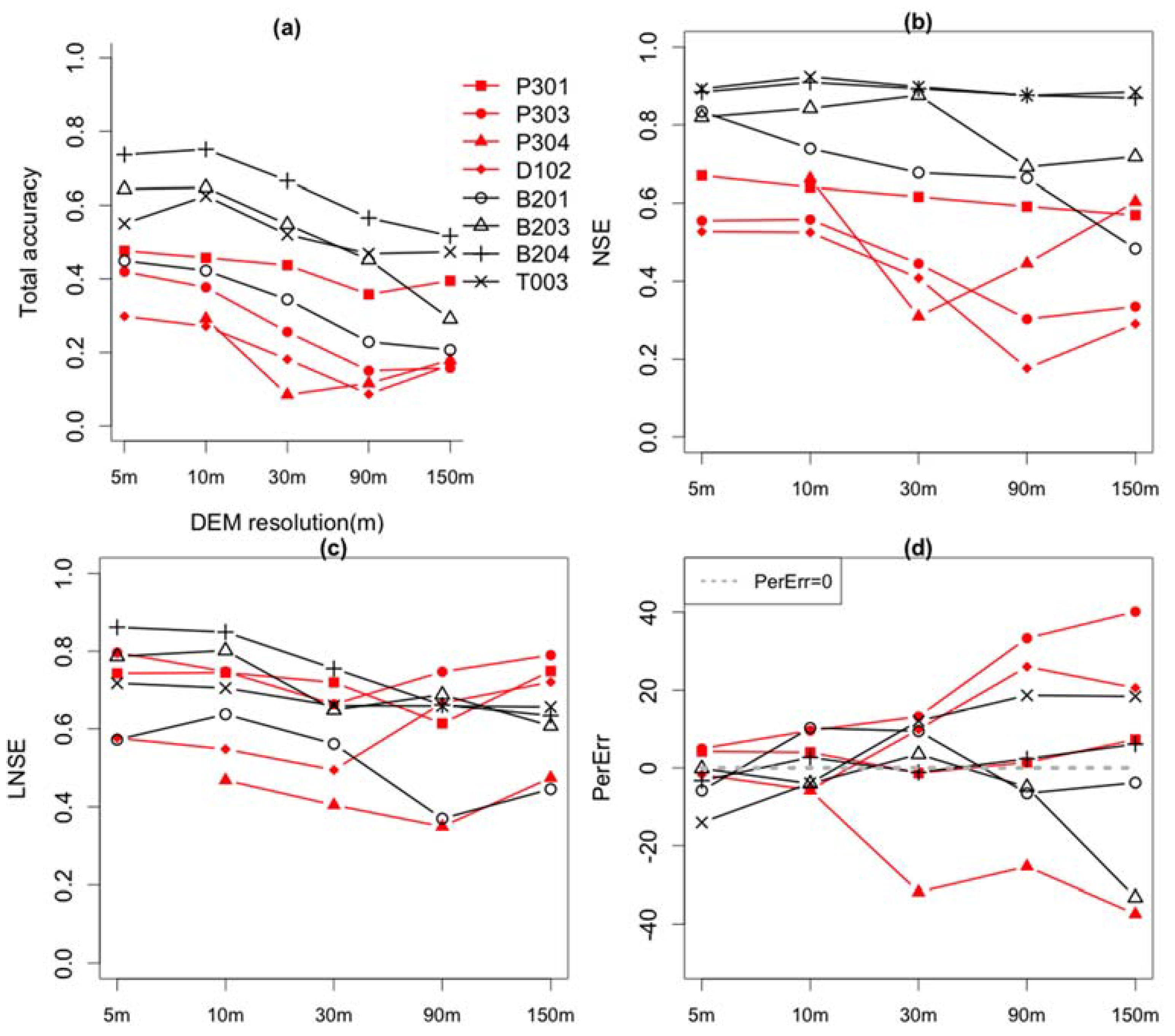
4.2. Effect of DEM Resolution on Streamflow Prediction Accuracy
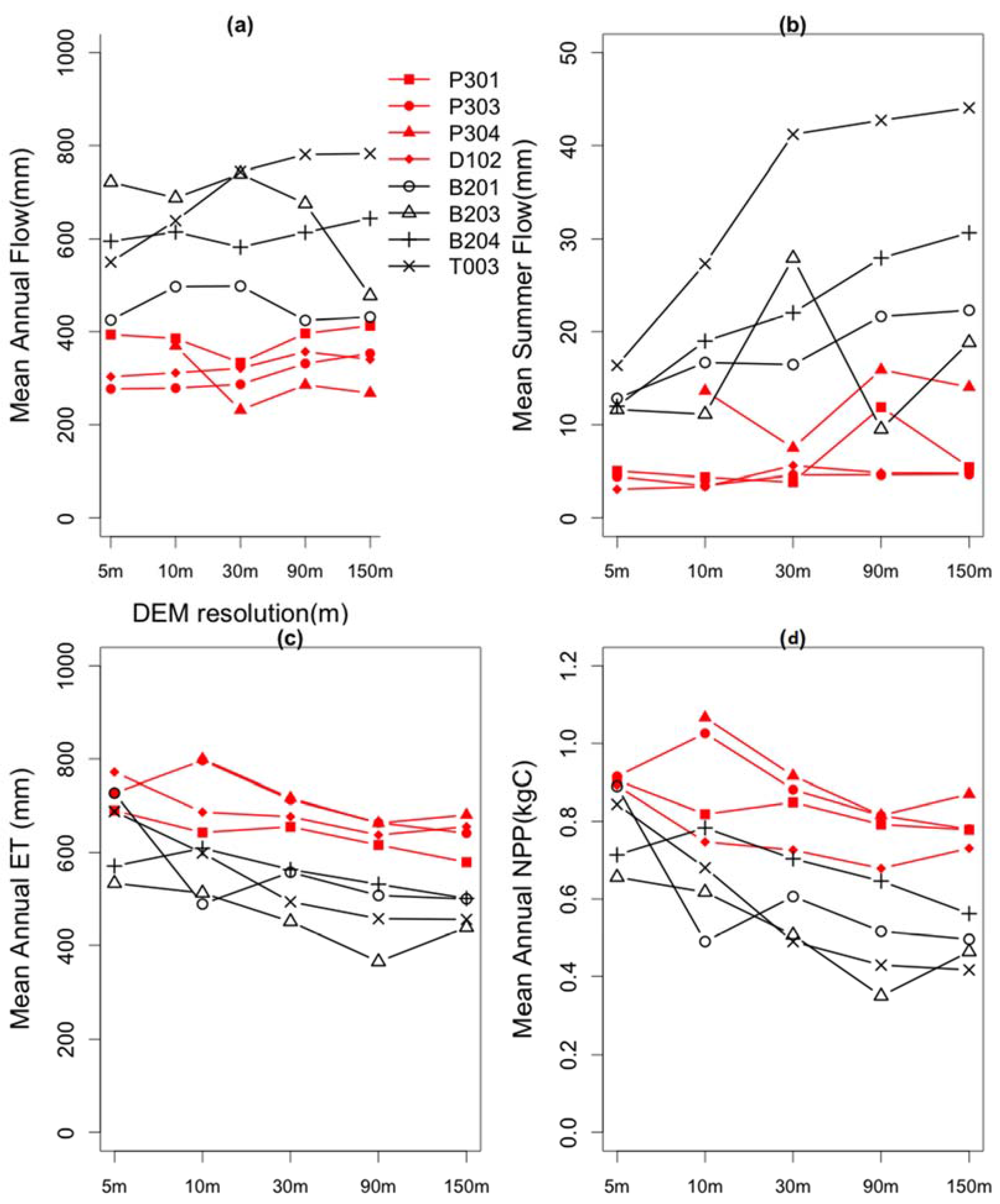
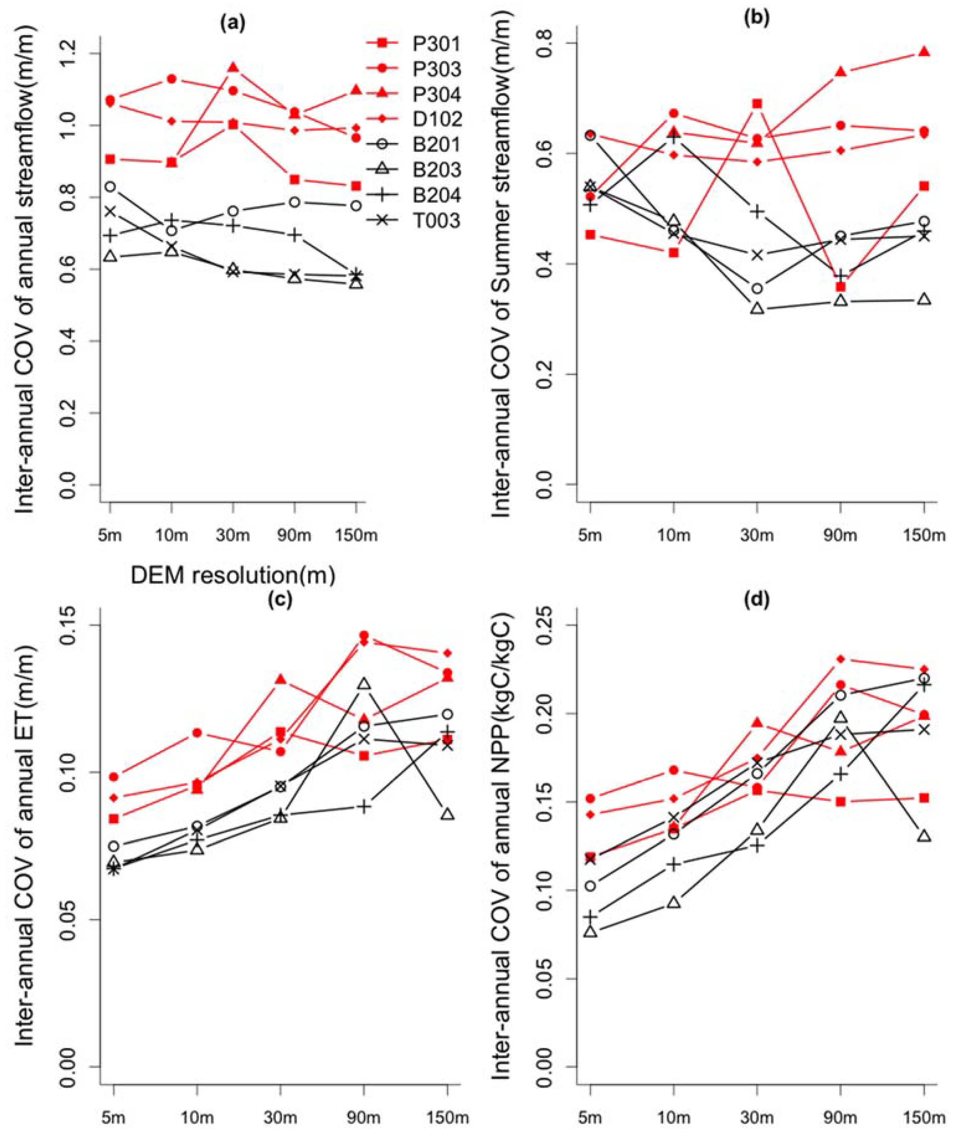
4.3. Sensitivity of Estimated Ecohydrologic Variables to DEM Resolution
5. Discussion and Summary
Acknowledgments
Author Contributions
Conflicts of Interest
References
- Knowles, N.; Cayan, D.R. Potential effects of global warming on the Sacramento/San Joaquin watershed and the San Francisco estuary. Geophys. Res. Lett. 2002, 29, 1891. [Google Scholar] [CrossRef]
- Maurer, E.; Duffy, P.P.B. Uncertainty in projections of streamflow changes due to climate change in California. Geophys. Res. Lett. 2005, 32, L03704. [Google Scholar] [CrossRef]
- Goulden, M.L.; Bales, R.C. Mountain runoff vulnerability to increased evapotranspiration with vegetation expansion. Proc. Natl. Acad. Sci. USA 2014, 111, 14071–14075. [Google Scholar] [CrossRef] [PubMed]
- Miller, N.L.; Bashford, K.E.; Strem, E. Potential impacts of climate change on california hydrology. J. Am. Water Resour. Assoc. 2003, 39, 771–784. [Google Scholar] [CrossRef]
- Null, S.E.; Viers, J.H.; Mount, J.F. Hydrologic response and watershed sensitivity to climate warming in California’s Sierra Nevada. PLoS ONE 2010, 5, e9932. [Google Scholar] [CrossRef] [PubMed]
- Zhang, W.; Montgomery, D.R. Digital elevation model grid size, landscape representation, and hydrologic simulations. Water Resour. Res. 1994, 30, 1019–1028. [Google Scholar] [CrossRef]
- Cline, D.; Elder, K.; Bales, R. Scale effects in a distributed snow water equivalence and snowmelt model for mountain basins. Hydrol. Process. 1998, 1536, 1527–1536. [Google Scholar] [CrossRef]
- Lassueur, T.; Joost, S.; Randin, C.F. Very high resolution digital elevation models: Do they improve models of plant species distribution? Ecol. Model. 2006, 198, 139–153. [Google Scholar] [CrossRef]
- Beven, K.J.; Kirkby, M.J. A physically based, variable contributing area model of basin hydrology/Un modèle à base physique de zone d’appel variable de l’hydrologie du bassin versant. Hydrol. Sci. Bull. 1979, 24, 43–69. [Google Scholar] [CrossRef]
- Kuo, W.; Steenhuis, T.S.; Mcculloch, C.E.; Mohler, C.L.; Weinstein, D.A.; DeGloria, S.D.; Swaney, D.P. Effect of grid size on runoff and soil moisture for a variable-source-area hydrology model. Water Resour. Res. 1999, 35, 3419–3428. [Google Scholar] [CrossRef]
- Musselman, K.N.; Molotch, N.P.; Brooks, P.D. Effects of vegetation on snow accumulation and ablation in a mid-latitude sub-alpine forest. Hydrol. Process. 2008, 22, 2767–2776. [Google Scholar] [CrossRef]
- Jost, G.; Weiler, M.; Gluns, D.R.; Alila, Y. The influence of forest and topography on snow accumulation and melt at the watershed-scale. J. Hydrol. 2007, 347, 101–115. [Google Scholar] [CrossRef]
- Chaubey, I.; Cotter, A.S.; Costello, T.A.; Soerens, T.S. Effect of DEM data resolution on SWAT output uncertainty. Hydrol. Process. 2005, 19, 621–628. [Google Scholar] [CrossRef]
- Mahmood, T.H.; Vivoni, E.R. Breakdown of hydrologic patterns upon model coarsening at hillslope scales and implications for experimental design. J. Hydrol. 2011, 411, 309–321. [Google Scholar] [CrossRef]
- Mo, X.; Liu, S.; Chen, D.; Lin, Z.; Guo, R.; Wang, K. Grid-size effects on estimation of evapotranspiration and gross primary production over a large Loess Plateau basin, China. Hydrol. Sci. J. 2009, 54, 160–173. [Google Scholar] [CrossRef]
- Tague, C.L.; Band, L.E. RHESSys: Regional hydro-ecologic simulation system—An object-oriented approach to spatially distributed modeling of carbon, water, and nutrient cycling. Earth Interact. 2004, 8, 1–42. [Google Scholar] [CrossRef]
- Hunsaker, C.T.; Whitaker, T.W.; Bales, R.C. Snowmelt runoff and water yield along elevation and temperature gradients in California’s Southern Sierra Nevada. JAWRA J. Am. Water Resour. Assoc. 2012, 48, 667–678. [Google Scholar] [CrossRef]
- Jefferson, A.J. Seasonal versus transient snow and the elevation dependence of climate sensitivity in maritime mountainous regions. Geophys. Res. Lett. 2011, 38. [Google Scholar] [CrossRef]
- Holmgren, P. Multiple flow direction algorithms for runoff modelling in grid based elevation models: An empirical evaluation. Hydrol. Process. 1994, 8, 327–334. [Google Scholar] [CrossRef]
- Running, S.W.; Nemani, R.R.; Hungerford, R.D. Extrapolation of synoptic meteorological data in mountainous terrain and its use for simulating forest evapotranspiration and photosynthesis. Can. J. For. Res. 1987, 17, 472–483. [Google Scholar] [CrossRef]
- Glassy, J.; Running, S. Validating diurnal climatology logic of the MT-CLIM model across a climatic gradient in Oregon. Ecol. Appl. 1994, 4, 248–257. [Google Scholar] [CrossRef]
- Coughlan, J.; Running, S. Regional ecosystem simulation: A general model for simulating snow accumulation and melt in mountainous terrain. Landsc. Ecol. 1997, 12, 119–136. [Google Scholar] [CrossRef]
- Thornton, P.E.; Running, S.W.; White, M.A. Generating surfaces of daily meteorological variables over large regions of complex terrain. J. Hydrol. 1997, 190, 214–251. [Google Scholar] [CrossRef]
- Monteith, J.L. Evaporation and environment. Symp. Soc. Exp. Biol. 1965, 19, 205–234. [Google Scholar] [PubMed]
- Jarvis, P.G. The interpretation of the variations in leaf water potential and stomatal conductance found in canopies in the field. Philos. Trans. R. Soc. B Biol. Sci. 1976, 273, 593–610. [Google Scholar] [CrossRef]
- Farquhar, G.D.; von Caemmerer, S.; Berry, J.A. A biochemical model of photosynthetic CO2 assimilation in leaves of C3 species. Planta 1980, 149, 78–90. [Google Scholar] [CrossRef] [PubMed]
- Ryan, M.G. Effects of climate change on plant respiration. Ecol. Appl. 1991, 1, 157–167. [Google Scholar] [CrossRef]
- Richardson, J.J.; Moskal, L.M.; Kim, S.-H. Modeling approaches to estimate effective leaf area index from aerial discrete-return LIDAR. Agric. For. Meteorol. 2009, 149, 1152–1160. [Google Scholar] [CrossRef]
- Dunn, S.M. Imposing constraints on parameter values of a conceptual hydrological model using baseflow response. Hydrol. Earth Syst. Sci. 1999, 3, 271–284. [Google Scholar] [CrossRef]
- Nash, J.E.; Sutcliffe, J.V. River flow forecasting through conceptual models part I—A discussion of principles. J. Hydrol. 1970, 10, 282–290. [Google Scholar] [CrossRef]
- Kenward, T.; Lettenmaier, D.P.; Wood, E.F.; Fielding, E. Effects of digital elevation model accuracy on hydrologic predictions. Remote Sens. Environ. 2000, 444, 432–444. [Google Scholar] [CrossRef]
- Hunsaker, C.; Neary, D. Sediment loads and erosion in forest headwater streams of the Sierra Nevada, California. In Proceedings of a Workshop Held during the XXV IUGG General Assembly in Melbourne, Melbourne, Australia, 28 June–7 July 2011.
- Liu, F.; Hunsaker, C.; Bales, R.C. Controls of streamflow generation in small catchments across the snow-rain transition in the Southern Sierra Nevada, California. Hydrol. Process. 2013, 12, 1959–1972. [Google Scholar] [CrossRef]
- Pradhan, N.R.; Ogden, F.L.; Tachikawa, Y.; Takara, K. Scaling of slope, upslope area, and soil water deficit: Implications for transferability and regionalization in topographic index modeling. Water Resour. Res. 2008, 44. [Google Scholar] [CrossRef]
- Wigmosta, M.S.; Vail, L.W.; Lettenmaier, D.P. A distributed hydrology-vegetation model for complex terrain. Water Resour. Res. 1994, 30, 1665–1679. [Google Scholar] [CrossRef]
- Tague, C.; Dugger, A. Ecohydrology and climate change in the mountains of the Western USA—A review of research and opportunities. Geogr. Compass 2010, 11, 1648–1663. [Google Scholar] [CrossRef]
- Dobrowski, S.Z. A climatic basis for microrefugia: the influence of terrain on climate. Glob. Chang. Biol. 2011, 17, 1022–1035. [Google Scholar] [CrossRef]


| Watershed | Watershed Mean Value of Topographic Parameters 1 | |||||
|---|---|---|---|---|---|---|
| Parameter | DEM Resolution | |||||
| 5 m | 10 m | 30 m | 90 m | 150 m | ||
| P301 | Elevation (m) | 1975.9 | 1976.6 | 1976.7 | 1975.5 | 1982.1 |
| Slope (°) | 12.3 | 11.9 *** | 10.7 *** | 9.2 *** | 7.8 *** | |
| Aspect 2 (°) | 258.8 | 259.0 | 256.5 | 256.3 | 266.6 | |
| Wetness (m) | 5.9 | 6.2 *** | 7.0 *** | 7.8 *** | 8.4 *** | |
| P303 | Elevation (m) | 1894.8 | 1894.5 | 1895.4 | 1890.9 | 1901.7 |
| Slope (°) | 14.0 | 13.7 *** | 12.6 *** | 11.6 *** | 10.7 *** | |
| Aspect 2 (°) | 214.4 | 214.9 | 214.4 | 212.4 | 218.2 | |
| Wetness (m) | 6.0 | 6.5 *** | 7.2 *** | 7.8 *** | 8.0 *** | |
| P304 | Elevation (m) | 1898.1 | 1896.8 * | 1898.1 | 1894.3 | 1905.5 |
| Slope (°) | 13.8 | 13.5 *** | 12.5 *** | 10.7 *** | 8.5 *** | |
| Aspect 2 (°) | 165.8 | 166.5 | 167.1 | 162.5 | 169.7 | |
| Wetness (m) | 5.9 | 6.2 *** | 6.8 *** | 7.7 *** | 8.0 *** | |
| D102 | Elevation (m) | 1772.0 | 1774.8 ** | 1772.8 | 1767.4 | 1785.4 |
| Slope (°) | 19.2 | 18.6 *** | 17.4 | 15.8 *** | 14.8 *** | |
| Aspect 2 (°) | 200.8 | 200.9 | 200.8 | 199.6 | 203.4 | |
| Wetness (m) | 5.7 | 6.1 *** | 6.9 *** | 7.6 *** | 7.7 *** | |
| B201 | Elevation (m) | 2253.8 | 2253.7 | 2254.4 | 2251.9 | 2248.4 |
| Slope (°) | 12.5 | 12.3 *** | 11.7 *** | 10.0 *** | 9.3 *** | |
| Aspect 2 (°) | 217.2 | 217.2 | 215.8 | 215.4 | 214.8 | |
| Wetness (m) | 6.3 | 6.5 *** | 6.9 *** | 7.7 *** | 7.9 *** | |
| B203 | Elevation | 2371.9 | 2371.6 | 2372.4 | 2372.7 | 2369.6 |
| Slope | 12.1 | 11.9 *** | 11.3 *** | 9.7 *** | 8.3 *** | |
| Aspect | 189.4 | 189.5 | 188.9 | 184.9 | 184.0 | |
| Wetness | 6.4 | 6.7 *** | 7.2 *** | 7.8 *** | 8.0 *** | |
| B204 | Elevation | 2360.3 | 2360.0 | 2360.7 | 2361.0 | 2357.3 |
| Slope | 12.1 | 11.9 *** | 11.1 *** | 9.0 *** | 8.2 *** | |
| Aspect | 178.2 | 177.8 | 176.7 | 173.2* | 172.6* | |
| Wetness | 6.3 | 6.5 *** | 7.0 *** | 7.8 *** | 8.4 *** | |
| T003 | Elevation | 2286.5 | 2287.0 | 2285.8 | 2283.2 | 2292.8 |
| Slope | 15.7 | 15.5 *** | 14.5 *** | 11.7 *** | 9.7 *** | |
| Aspect | 304.0 | 304.1 * | 305.1 *** | 309.3 *** | 308.8 *** | |
| Wetness | 6.0 | 6.2 *** | 6.6 *** | 7.4 *** | 8.2 *** | |
| Watershed | Snow-Related Parameters | Model Accuracy of Snow Predictions | |||
|---|---|---|---|---|---|
| Temperature Lapse Rates 1 (tmax/tmin) (°C/m) | Temperature Threshold for Rain vs. Snow 2 (°C) | Temperature Melt Coefficient 3 (m/°C) | Day of Snow Melt 4 | SWE 5 | |
| Providence | 0.0063/−0.0064 | −3-3 | 0.005 | 0.92 | 0.91 |
| Bull | 0.0068/−0.0060 | −3-3 | 0.005 | 0.83 | 0.83 |
| Watershed Group | Watershed | Change in Spatial Variance of Wetness Index (%) | Change in Streamflow Accuracy (Equation (4)) (%) | Model-Based Rank 5 |
|---|---|---|---|---|
| TSWs | P301 | −9 1 (3) 2 | −25 3 (−14) 4 | 7 |
| P303 | −31 (−14) | −64 (−44) | 3 | |
| P304 | −1 (5) | −71 (−42) | 1 | |
| D102 | −26 (−11) | −71 (−41) | 2 | |
| SDWs | B201 | −5 (−1) | −54 (−33) | 5 |
| B203 | −4 (11) | −55 (−25) | 4 | |
| B204 | 7 (12) | −30 (−15) | 6 | |
| T003 | 11 (25) | −15 (−5) | 8 |
© 2016 by the authors; licensee MDPI, Basel, Switzerland. This article is an open access article distributed under the terms and conditions of the Creative Commons Attribution (CC-BY) license (http://creativecommons.org/licenses/by/4.0/).
Share and Cite
Son, K.; Tague, C.; Hunsaker, C. Effects of Model Spatial Resolution on Ecohydrologic Predictions and Their Sensitivity to Inter-Annual Climate Variability. Water 2016, 8, 321. https://doi.org/10.3390/w8080321
Son K, Tague C, Hunsaker C. Effects of Model Spatial Resolution on Ecohydrologic Predictions and Their Sensitivity to Inter-Annual Climate Variability. Water. 2016; 8(8):321. https://doi.org/10.3390/w8080321
Chicago/Turabian StyleSon, Kyongho, Christina Tague, and Carolyn Hunsaker. 2016. "Effects of Model Spatial Resolution on Ecohydrologic Predictions and Their Sensitivity to Inter-Annual Climate Variability" Water 8, no. 8: 321. https://doi.org/10.3390/w8080321
APA StyleSon, K., Tague, C., & Hunsaker, C. (2016). Effects of Model Spatial Resolution on Ecohydrologic Predictions and Their Sensitivity to Inter-Annual Climate Variability. Water, 8(8), 321. https://doi.org/10.3390/w8080321