1. Introduction
In recent years, Taiwan has been under the influence of global warming because of the frequent extreme climatic conditions and the disasters caused by typhoons and heavy rains. Hydrological observation operations, and the collection and analysis of the related information have been critical in facilitating disaster prevention, and the response, management, and planning of the rivers. The collection and analysis of hydrological data can provide important references for the allocation and utilization of water resources, disaster prevention and warning, and the development of various supply and demand plans for water, as well as the planning and design of hydraulic engineering projects. The topographic conditions of the rivers in Taiwan are slightly unusual, including steep slopes and rapid streams. Floods that are heavy with sand occur, whenever torrential rainfall and typhoons occur. Thus, the erosion and deposition at the cross section of the rivers and the flow path change significantly, making flow observation a difficult task. In addition, most rivers have various river crossing and flood-control constructions, such as bridges, consolidation works, submerged weirs, and river weirs, and the physical change in the water caused by such man-made interferences can affect the precision of the measured data. However, it is worth mentioning that these structures may also represent good, or even optimal, locations for stream gauging because the weirs impose a fixed bed topography and the bridges facilitate the acquisition of data along a cross-section. Therefore, a knowledge of the accurate flow of the rivers is crucial for planning and utilizing water resources and for designing the associated works.
Flow observation includes the observation of the water depth and the flow velocity; they have to be mostly conducted manually and are time-consuming, strenuous, dangerous, and have low precision; however, the precision (and accuracy) is influenced by various other factors. Currently, there are no instruments employed for automatic observation at home and abroad that are suitable for evaluating the environmental conditions of the rivers in Taiwan. Thus, investigations can only be made indirectly by hydrological models. All of the instruments for the water depth observation, such as the conventional sounding rod, heavy punch, and fish lead to a sounding boat equipped with ultrasonic detectors; the acoustic Doppler current profiler (ADCP) and ground penetrating radar (GPR) used for measuring the water depth require manual field operations and are do not support automatic observation. Instruments used for the flow velocity observation, such as those using the conventional float method, the cup-type current meter, propeller-type current meter, electromagnetic current meter, acoustic Doppler current profiler, and the radar surface current meter (which is currently used) already have the capability for automatic observation. In addition, the optics-based methods that are rapidly emerging may provide useful velocity benchmark values for future radar investigations. These methods also utilize the images for identifying the river flow, e.g., large-scale particle image velocimetry (LSPIV) [
1,
2,
3].
As all the microwave radar surface current meters are imported, the measurement results are obtained by the instruments directly and the firmware program cannot be changed. Thus, there are only a limited number of adjustable setup parameters in the instruments and the measurement results cannot be processed further in the form of signals. Thus, a continuous wave radar surface current meter with automatic observation was adopted in this study to analyze the radar signals received by the instruments. The surface velocity was estimated using the conventional fast Fourier transform (FFT), wavelet transform (WT), and a bandpass filter to seek an effective method suitable for real-time observations for analyzing the signals and the uncertainties related to the radar-based flow velocity estimations.
2. Literature Review
The radar surface current meter includes a pulsed Doppler radar and a continuous microwave radar. Melcher
et al. [
4] mounted a pulsed radar on a helicopter and Cheng
et al. [
5] mounted a pulsed radar on a riverbank to measure the surface velocity of the entire cross-section at different locations and distances by adjusting the tilt angle; however, it still required manual operations. The continuous microwave radar can be placed on cross-river constructions. A single such instrument can measure an elliptical footprint, while multiple instruments can measure the surface velocity of the entire cross section and it can be used directly for automatic measurements without manual operation; e.g., Costa
et al. [
6] mounted a pulsed radar on the riverbank and a continuous wave radar was deployed from a cableway or installed under a bridge.
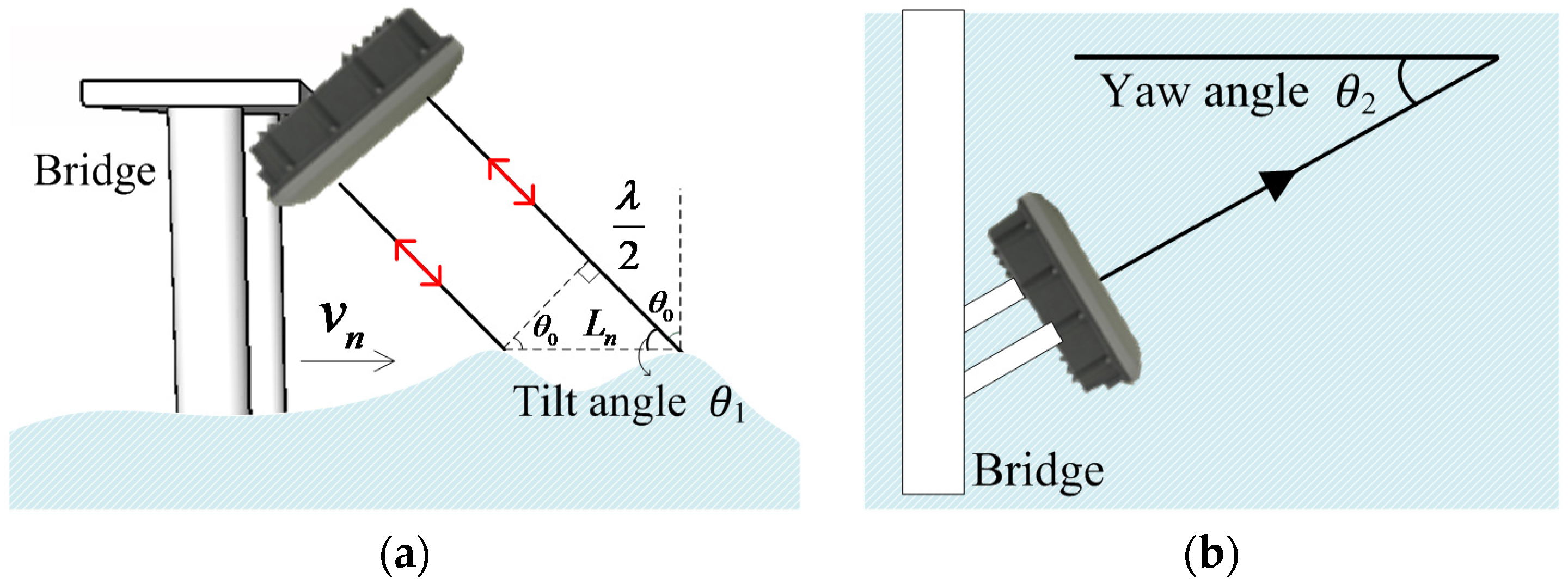
The continuous microwave radar surface current meter calculates the surface velocity of the river by using the Bragg scattering and the Doppler shift of the reflection of the radar waves, caused by tiny ripples on the stream surface. Therefore, the setup of the tilt angle (the angle between the horizontal plane and the direction of the radar wave transmission) and the yaw angle (the angle between the mainstream direction and the direction of the radar wave transmission) affect the measurement results of the surface velocity apart from the influence of the stream conditions of the rivers. Limited by environmental factors, the measurement direction is not guaranteed to be in parallel with the mainstream direction; thus, the reflected waves received by the microwave radar may not be reflected by the ripples moving in the mainstream direction. A Doppler radar instrument enables the calculation of the component of the velocity vector of the target along the beam. Unless the beam is parallel to the main flow velocity (tilt angle and yaw angle, both equal to zero), this component differs from the actual flow velocity. While the drift angle can be zero (for example, if the instrument is placed on a bridge), the depression angle is always larger than zero for a non-contact water survey setup but, in both the cases, their effect can be calculated using trigonometric relationships.
When a yaw angle (horizontal included angle) exists between the measurement direction and the mainstream direction, the calculation formula for the surface velocity can be revised by the yaw angle; when the angle is considerably large, the measurement results may not give an exact value for the surface velocity along the mainstream direction. The tilt and the yaw angle have the same type of effect on the measurements as they represent the angle between the radar beam and the flow velocity on two different planes. Trigonometric corrections can be applied either on-the-fly or during data post-processing in both cases.
Hsu
et al. [
7] conducted measurements on the surface velocity with a propeller-type current meter and a 10.525 GHz microwave radar current meter having a tilt angle range of 20–60 degrees and a yaw angle range of 0–40 degrees. The results indicated that the standard deviation of the measurement results obtained by the radar wave current meter were larger than those obtained by the propeller-type current meter. Therefore, when measuring the surface velocity with the radar wave current meter, the signals received by the radar waves of this instrument should be analyzed in addition to the settings according to the original correction parameters and the measurement direction should be in line with the positive flow direction as much as possible in order to avoid the yaw angle correction. If correcting the yaw angle becomes necessary, then the corrected angle should be controlled within 20 degrees to improve the precision of the observation results of the surface velocity [
7]. Lee and Julien [
8] compared some of the laboratory tests with the field tests and demonstrated satisfactory agreements over a wide range of tilt and yaw angles. Laboratory testing showed comparable results between the electromagnetic wave surface velocimeters and other measurement techniques. Field testing at three different locations show that the optimal operation conditions are at a tilt angle of approximately 30 degrees and a yaw angle less than 13 degrees.
Previous studies seldom focus on the noise removed by the radar echo signals and most of them discuss the measurement results with different radar wave transmitting antennae or erections of instruments. Costa
et al. [
9] utilized van-mounted, pulsed Doppler (10 GHz) radar collected surface-velocity data across the 183-m wide Skagit river in Washington at a USGS stream gaging station using Bragg scattering from the short waves produced by turbulent boils on the surface of the river. Melcher
et al. [
4] indicated that the United States Geological Survey and the University of Washington collaborated in a series of initial experiments on the Lewis, Toutle, and Cowlitz Rivers during September 2000 and in a detailed experiment on the Cowlitz River during May 2001 for determining the feasibility of using helicopter-mounted radars for measuring the river discharge (surface velocities were measured using a pulsed Doppler radar). Tamari
et al. [
10] tested a handheld radar to measure the water velocity at the surface of the channels, while Kim
et al. [
11] analyzed the error in the electromagnetic surface velocity and discharge measurement in a rapid mountain stream flow. Therefore, rapid and effective processing, and the method used for analyzing the surface current meter signals, are key issues.
The optimal linear filtering theory, also called the Wiener filtering theory, was derived from the study of Kolmogorov [
12] and Wiener
et al. [
13]. The greatest disadvantage of the Wiener filtering theory is that it requires data from the infinite past and it is not applicable for time series processing. To overcome this disadvantage, Kalman [
14] introduced a state-space model in the filtering theory and deduced a recursive estimation algorithm called the Kalman filtering theory. Kalman filtering adopts the minimum mean square error as the optimum criterion to obtain a recursive estimation algorithm. It updates the estimation of the state variables by the estimated value at the last instance in time and the observed value at present with the state-space model of the signal and noise to obtain the estimated value at present. Another method similar to the Kalman filtering is the adaptive filter [
15,
16,
17]; however, its filter coefficient can vary depending upon certain requirements at any given point in time. The adaptive filter is often adopted when the optimal coefficient of the digital filter cannot be determined. If an adaptive filter is adopted along with the noise elimination system, noise will inevitably be mixed with the signals received by the sensors [
18]. Therefore, sometimes two sensors may be adopted for reducing the noise interference, with one mainly detecting the target signals and the other detecting the noise. When a surface current meter is placed on site, the space for storing the component information is limited; all of the above filters perform a significant number of calculations; hence, they are suitable for systems with a large storage space (such as computers). Therefore, this study compares the errors in the various methods used for estimating the surface velocity, via wavelet transform and a bandpass filter that calculate rapidly and do not depend upon previous measurement information, apart from the fast Fourier transform method, necessary for the calculations.
3. Hydrologic Signal Processing Approach
The principle for measuring the surface velocity using a microwave radar surface current meter is derived from the Bragg scattering and the Doppler effect. When the wavelength of the radar waves incident on the water surface are 2n times that of the waves on the water surface, the radar waves generate a Bragg scattering (as shown in
Figure 1) owing to interaction with the waves on the water surface, causing resonance. The Bragg resonance yields a Doppler shift when the ripples move on the water surface; thus, the movement speed of the ripples, namely, the surface velocity of the water body, can be obtained using the Doppler shift.
Bragg scattering is shown in
Figure 1.
is the Bragg resonance wavelength,
is the wavelength of the radar waves, and
is the incidence angle of the radar waves. Their relationship can be expressed as follows [
19]:
According to the Doppler effect,
is the speed of the surface ripples moving towards/away from the microwave radar surface current meter; thus, the Doppler peak frequency of the echo Doppler spectrum,
, Can be expressed as follows [
19]:
In the above formula,
is the line-of-sight velocity,
i.e., the component of the scattered velocity along the antenna direction.
Figure 1 shows the method for measuring the surface velocity of a river, when a microwave radar surface current meter is placed at a fixed location (such as bridge) and the formula for calculating the surface velocity is as follows:
In the above formula, is the surface velocity of the water body, is the speed of the radar waves transmitting in air (3 × 10⁸ m/s), is the frequency of the microwave radar antennae (10.525 GHz), is the Doppler peak frequency caused by the movement of the surface ripples, is the tilt angle, is the yaw angle, and is the angle between the radar waves and the flow direction. The transmission speed of the radar waves, , the frequency of the radar antennae, , and the angle between the radar waves and the flow direction, , are known constants; hence, the surface velocity, , can be estimated by measuring the receiving frequency of the radar echo, . Therefore, the precision of the radar echo frequency, , is very important in estimating the surface velocity of a river.
In practice, the influence of the ripples generated by the wind and rain on the water surface on the radar echo signals cannot be determined using only conventional fast Fourier transform. To discuss the applicability and feasibility of the different analyses methods for the flow velocity signals, trolley tests were conducted in this study at the Laboratory of Current Meter Calibration of the Water Resources Planning Institute, Ministry of Economic Affairs. The original signals of the microwave radar surface current meter were measured and analyzed by fast Fourier transform, wavelet transform, and a bandpass filter. Further, the precision in estimating the surface velocity by these three analytical methods was compared to determine an effective method that would be suitable for real-time observations for identifying the radar wave frequency.
3.1. Fast Fourier Transform
In the past, the corresponding frequency spectrum (frequency-amplitude) of the signals was obtained by discrete Fourier transform (DFT) for analyzing signals to obtain their important parameters. As the number of calculations were significant, the discrete Fourier transform required considerable time for the calculations; hence, it was difficult to obtain results in real-time. Cooley and Tukey [
20] simplified the discrete Fourier transform and employed the fast Fourier transform that improved the calculation speed significantly and it was widely adopted in various fields; however, it has certain limits: (1) periodic signals are required; (2) the sampling period must be an integral multiple of the signal period; (3) the sampling frequency must be at least two times higher than the maximum frequency of the signals; and (4) the length of the sampling information must be in powers of two.
Conventionally, the estimation of the receiving frequency of the radar echo,
, is conducted using the fast Fourier transform for analyzing the original radar echo signals (as shown in Equation (4)) and for determining the resonant peak frequency of the power spectral density (PSD) to obtain the Doppler peak frequency,
(as shown in Equation (5)).
In the above formula, represents the original measured signals, represents the sample frequency (Hz), the range – indicates the measurement time, represents the amplitude, represents the power spectral density, and is the maximum amplitude of , corresponding to the frequency. As radar waves transmit rapidly and receive signals sensitively, echo signals often carry noise that directly affect the estimated value of the Doppler peak frequency, . Further, as the flow velocity signal information is a time-varying signal, the information on only a part of the time domain only can be obtained if it is analyzed by fast the Fourier transform and the power spectral density (PSD). This is unsuitable for the nonlinear and unsteady information on the rivers because the noise signal cannot be distinguished from the master signal. Therefore, the wavelet transform was adopted in this study for signal analysis to filter the noise.
3.2. Wavelet Transform
The basic wavelet function is called the mother wavelet and the wavelets generated by extension, contraction, and translation are defined as baby wavelets [
21,
22,
23,
24,
25,
26,
27]. The mother wavelet function must meet the following two requirements:
- 1.
The energy of the mother wavelets must be finite, as shown in Equation (6):
In the above formula, stands for the energy of the mother wavelet and stands for the mother wavelet function.
- 2.
Mother wavelets must meet the admissible conditions, as shown in Equation (7):
In the above formula, stands for the admissible constant that varies slightly depending upon the wavelets. Equation (7) is called the admissibility condition and is the Fourier transform of .
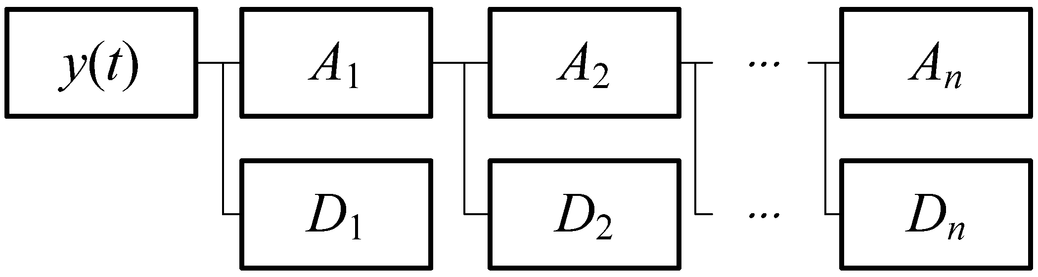
From the signal analysis perspective, any signal can be considered as a multi-frequency signal function and a compound of signals with different resolutions by linear additivity. The conventional Fourier transform can only present a single signal in the time domain or frequency domain, while the signals can extract the required information from the original signals after being processed by the wavelet transform. Multi-scale analysis by the scale extension and translation operation functions is conducive for the enhancement and identification of the signal characteristics, and the analysis of nonlinear and unsteady information. This implies that the wavelet transform decomposes an original signal into a combination (as shown in
Figure 2) of approximation signals (represented by A) and detail signals (represented by D), as shown in Equation (8):
In the above formula, represents the original signal, represent the detail signals from the decomposition of the original signal by the wavelet transform, represents the approximation signals, and represents the order of the wavelet decomposition.
Signal composition follows the decomposition of the original signal into detail signals and approximation signals with different composition methods corresponding to different properties of the original signal that can then be divided into detail signal compositions (as shown in Equation (9)) and approximation signal compositions (as shown in Equation (10)). Donoho [
28] and Misiti
et al. [
25] adopted the detail/approximation signal composition infinitely to filter signals with a set threshold value. Taswell [
29] proposed the elimination of the noise in the original signal by composing only the approximation signals; however, the tests in the study indicated that the approximation signals were only suitable for low flow velocity (under 1.0 m/s) analyses, while the detail signals were required for those above 1.0 m/s. In practical applications, it is difficult to set the filter for automatically compounding the detail/approximation signals, given that the onsite flow velocity cannot be determined. By considering the importance of the flow velocity information, in this study, detail signals were adopted for the wavelet signal composition to obtain the velocity information.
where
is the composition of the detail signals and
is the composition of the approximation signals. The Daubechies wavelet function used in this study, was adopted as the wavelet transform filter and the dmey function (discrete approximation of the Meyer wavelet) of MATLAB was employed for decomposing the wavelet into five detail signals and one approximation signal. It is difficult for the wavelet signals to set the filter for an automatic switchover between the compositions of the detail/approximation signals; moreover, the different numbers of the decomposed signals can affect the differences in the composed signals. Therefore, a bandpass filter was adopted to conduct an additional signal analysis to filter the noise.
3.3. Bandpass Filter
A filter discards the unnecessary low frequency (or high frequency) parts of a complex signal and ensures that most of the passed high-frequency (or low-frequency) signals are useful; the definitions of the low-frequency and high-frequency are determined by the cut-off frequency selected by the designer of the filter. A pure filter can be divided into a high-pass filter, low-pass filter, and a bandpass filter. A high-pass filter allows the passage of high-frequency signals but weakens (or reduces) signals whose frequency is lower than the cut-off frequency; on the contrary, a low-pass filter allows the passage of low-frequency signals but weakens (or reduces) the signals whose frequency is above the cut-off frequency. However, both low-frequency and high-frequency signals (low flow velocity and high flow velocity) can be encountered during the identification of the radar wave surface velocity owing to the interference of the external environmental conditions. Therefore, in this study, a bandpass filter that integrates both high- and low-pass filtering should be applied to the microwave radar surface current meter instead of a pure high-pass filter or a pure low-pass filter.
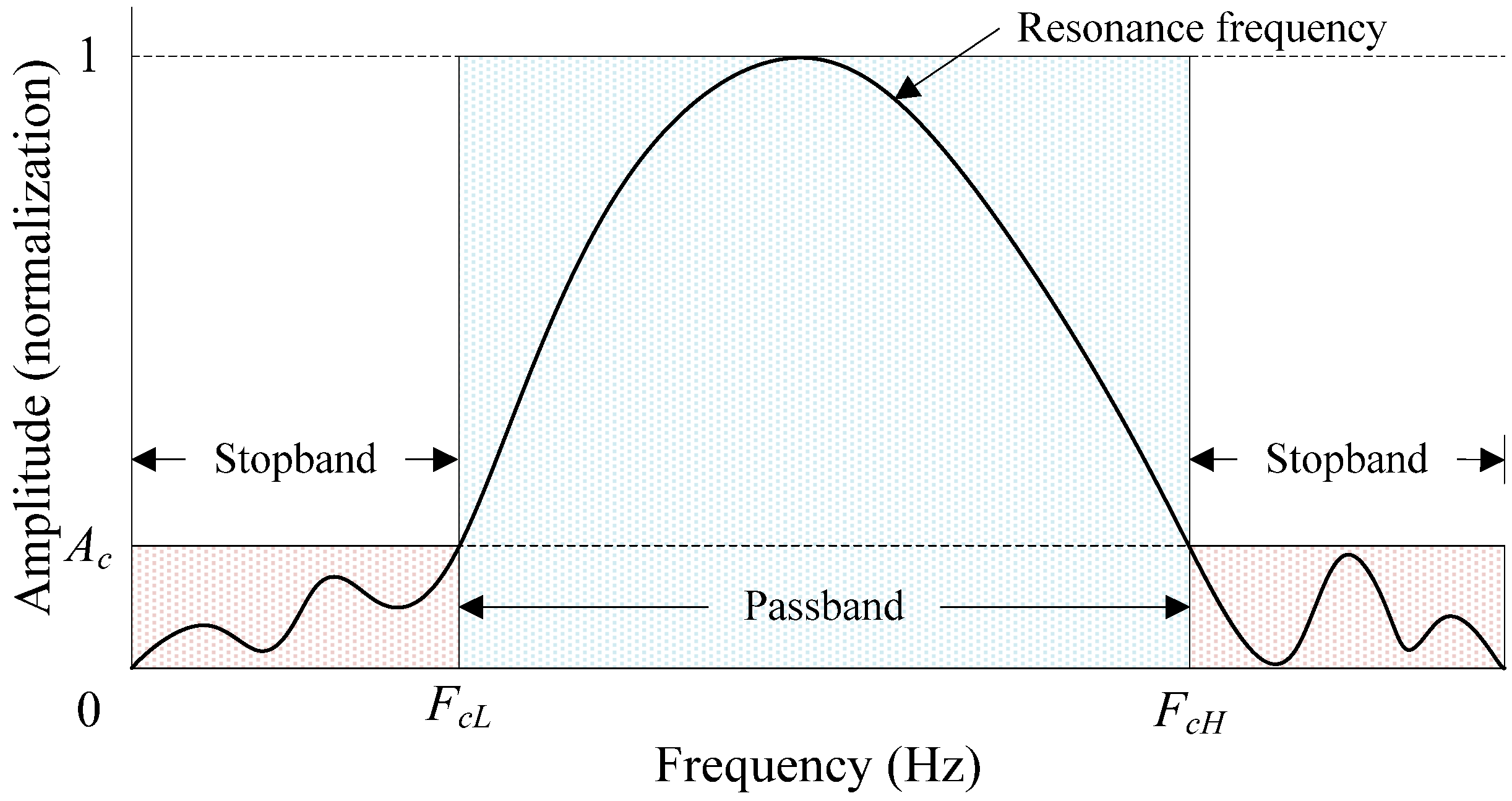
An ideal bandpass filter has a completely flat passband (
i.e., with no gain/attenuation throughout) and will completely attenuate all the frequencies outside the passband. Additionally, the transition out of the passband will have brick-wall characteristics [
30], as shown in
Figure 3. The resonance frequency is the difference between the cut-off frequency,
FcL, of a lower frequency band and the cut-off frequency,
FcH, of a higher frequency band; the bandpass width of the filter is the difference between
FcL and
FcH.
To extract each modal signal from a given signal, a digital bandpass stopband filter that contains one to several modal frequencies for a signal was designed.
Figure 3 illustrates the design map of a filter that uses a cutoff frequency corresponding in amplitude to 10% of the peak value (
i.e.,
Ac = 0.1) of the signal in the frequency spectrum [
31,
32]. The signal was only allowed oscillation between the stopband cutoff frequencies (
i.e.,
FcL–
FcH), and the amplitudes in the other intervals (
i.e., 0–
FcL and higher than
FcH) were set to zero to filter out the lower and higher portions of the signal, arising from the measurement errors.
4. Experimentation and Analysis
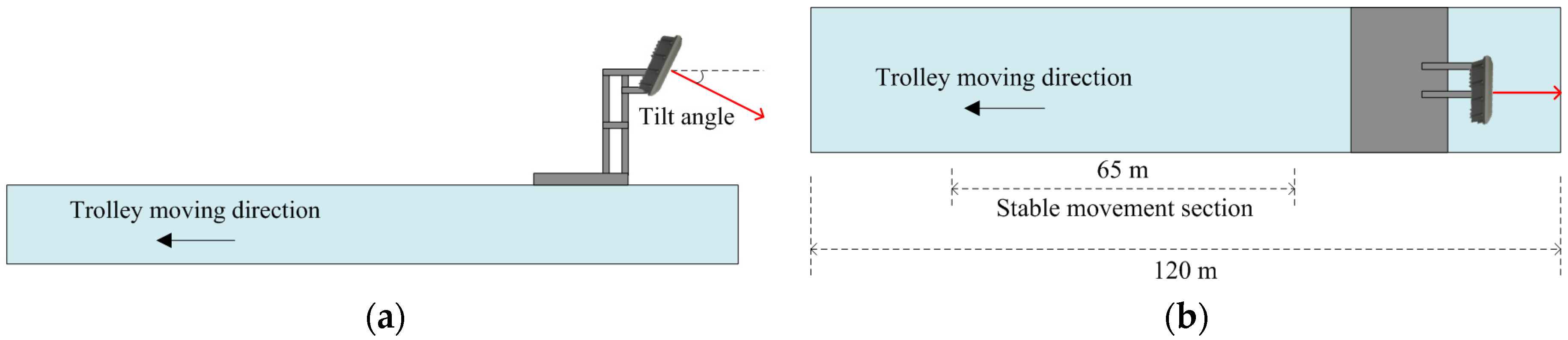
A 10.525 GHz microwave radar surface current meter (test model before the product development, resolution: 0.01 m/s, voltage: 12–36 VDC, temperature: −35–60 °C, ingress protection: 65) was adopted. The experiments were conducted at the Laboratory of Current Meter Calibration of the Water Resources Planning Institute, Ministry of Economic Affairs that is the only current meter calibration laboratory approved by the Taiwan Accreditation Foundation (TAF). The calibration trolley in the laboratory has a calibration speed of 0.3–6.0 m/s, minimum uncertainty of 2%, and a minimum speed of 0.2 m/s. The length and width of the experimental channel are 120 m and 1.6 m, respectively. The trolley initially advances slowly, accelerating gradually and moves at a constant speed when it reaches the set location (start of the stable movement section). It then decelerates and ultimately stops after moving for 65 m in the stable movement section. The instrument is fixed on the stainless steel shelf on the trolley for the measurement (as shown in
Figure 4). The water surface is still during the measurement, and ripples appear on the water surface as the trolley moves; therefore, the radar wave reflected signals could be measured for calculating the errors incurred by the different analytical methods, while identifying the surface velocity and the actual movement speed of the trolley, as shown in Equation (11):
where
is the relative error (%),
is the identification result of the surface velocity (m/s), and
is the actual movement speed of the trolley (m/s).
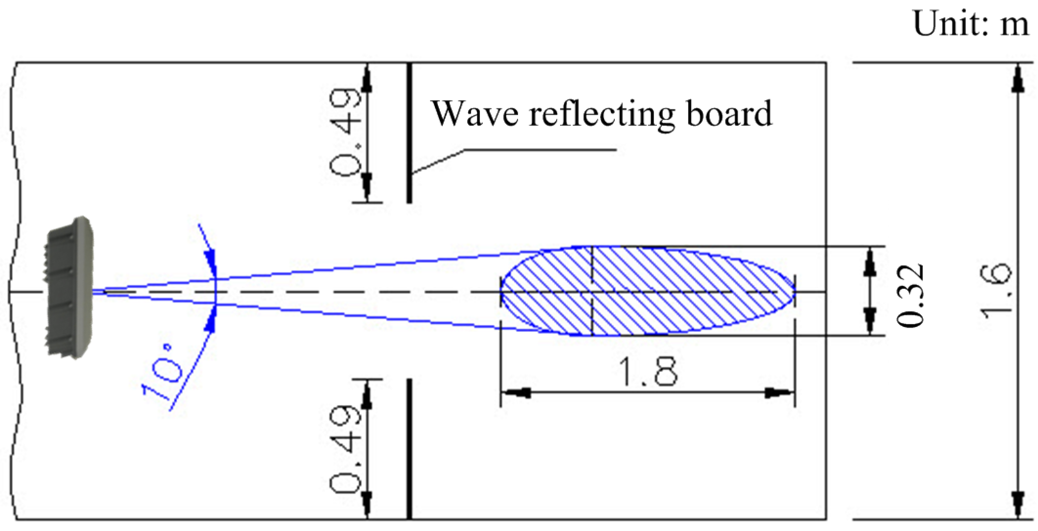
Herein, the incident direction of the radar waves and the flow direction are mostly parallel (namely, yaw angle = 0 degrees); therefore, this study discusses the differences between the different analytical methods for the identification of the surface velocity under varying flow velocities and incident tilt angles. The tilt angle for the experiments in this study was set as 20, 30, 40, 50, and 60 degrees; the movement speed of the trolley was 0.2, 1.0, 1.5, 2.0, 2.5, 3.0, 4.0, 5.0, and 6.0 m/s; the incident direction of the radar waves was opposite to the movement direction of the trolley,
i.e., the simulated incident direction of the radar waves was the same as the stream direction. A total of 45 sets of experiments were conducted. The surface current meter in this study was set to a continuous measurement and a group of data was obtained every 2 s; each group contained 640 data points and each data point had a measurement interval of
s; the frequency of the samples was 2.34 kHz. The range of the radar emission angle was 10 degrees and the radar emission position was 1.04 m above the water surface; the width of the illuminated area was approximately 0.11–0.50 m (tilt angle 20–60 degrees) that was 1.6 m narrower than the width of the channel; it is necessary to ensure that the sample is not affected by the presence of the side walls (as shown in
Figure 5).
For example, the original signals of the radar waves are shown in
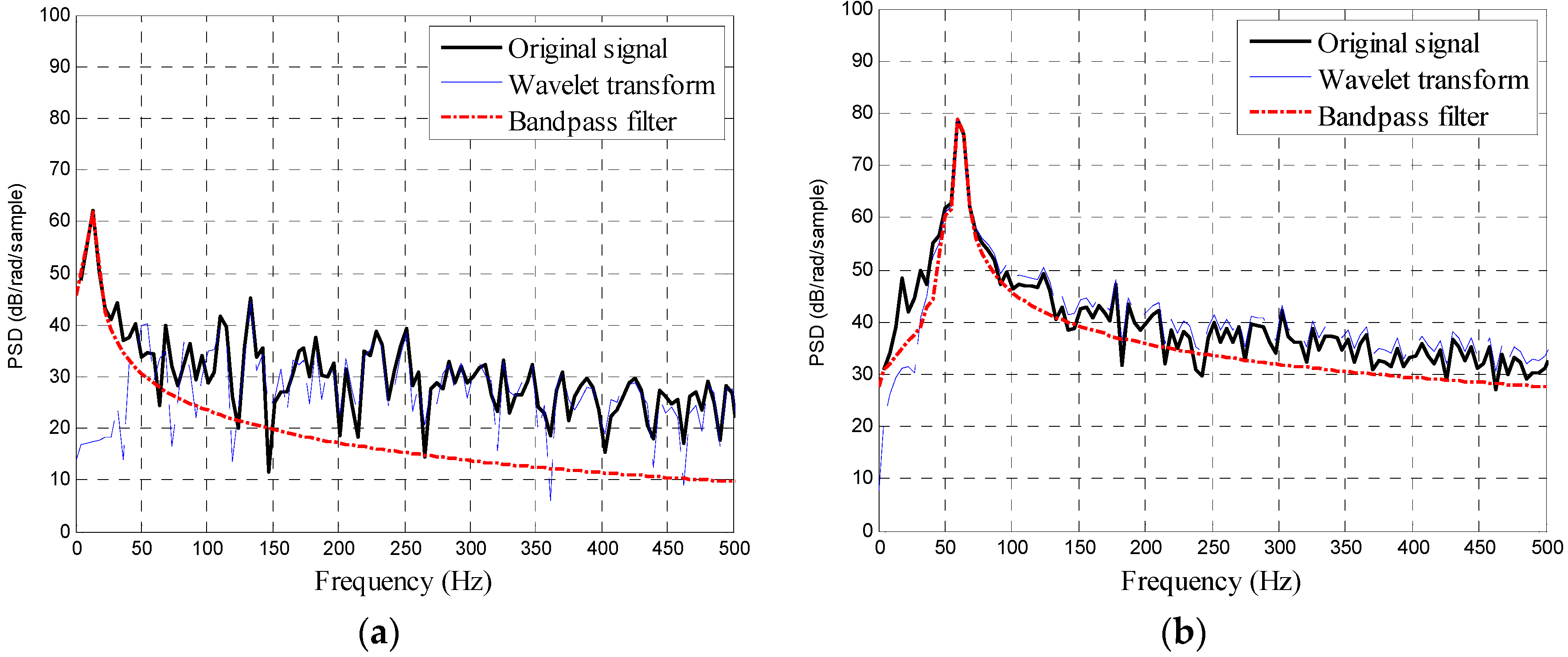
Figure 6 and the original signals (by conventional FFT only), wavelet analysis, and the signal frequency spectrum after the bandpass filter analysis are shown in
Figure 7, when the tilt angle is 30 degrees, and the speed of the trolley is 0.2 m/s and 1.0 m/s. According to
Figure 7, there is considerable noise (several peak frequencies) in the original signals. The noise that can be filtered by the wavelet transform is negligible, often resulting in interference and misjudgment of the peak frequency, while the bandpass filter can filter the redundant noise for representing the frequency spectrum chart as a smooth curve. Thus, the peak frequency can be easily identified.
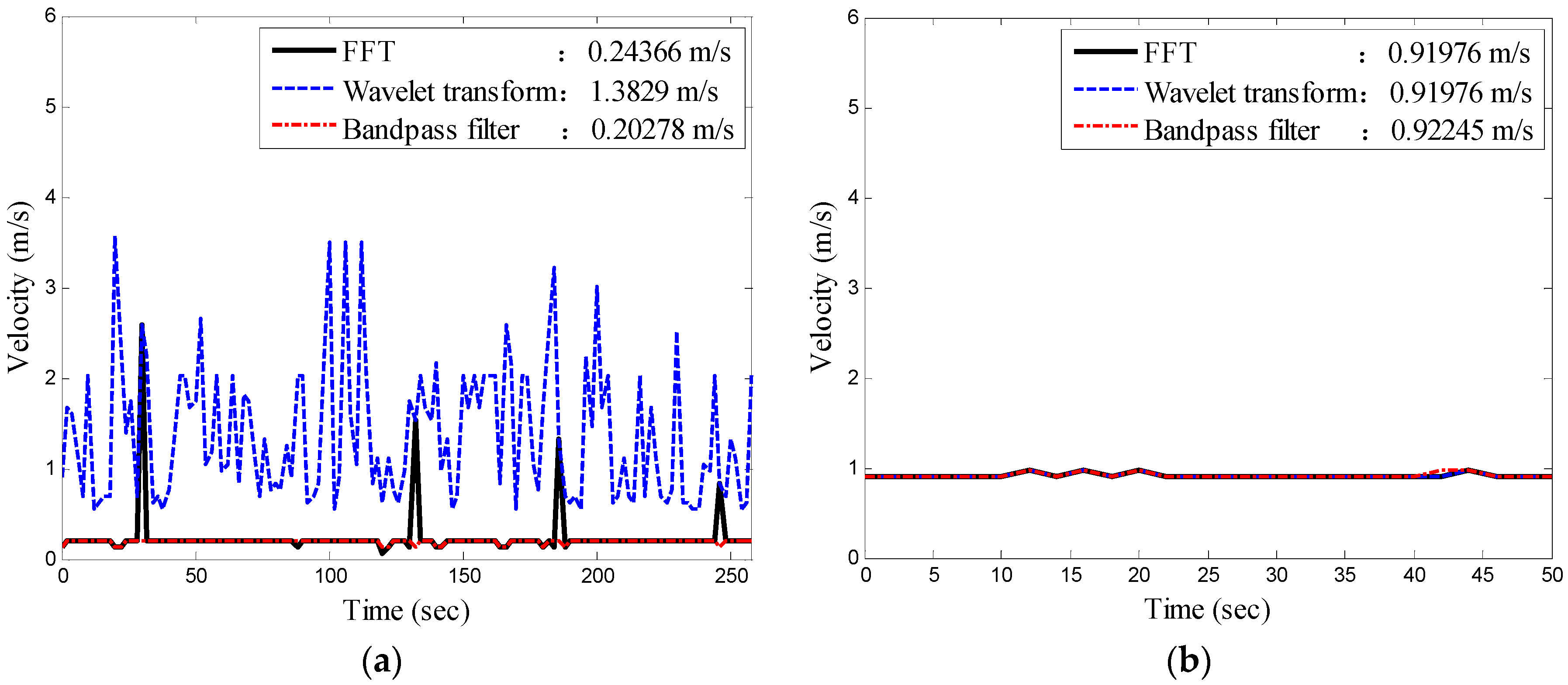
Figure 8 shows the results of the flow velocity obtained using the three methods. The calculation of the flow velocity using the original signals was unstable and fluctuated because of considerable noise. The calculation of flow velocity using the wavelet analysis was slightly more stable, but it often misjudged the peak frequency, while the calculation of the flow velocity using the bandpass filter was stable and the identification results were closer to the actual values.
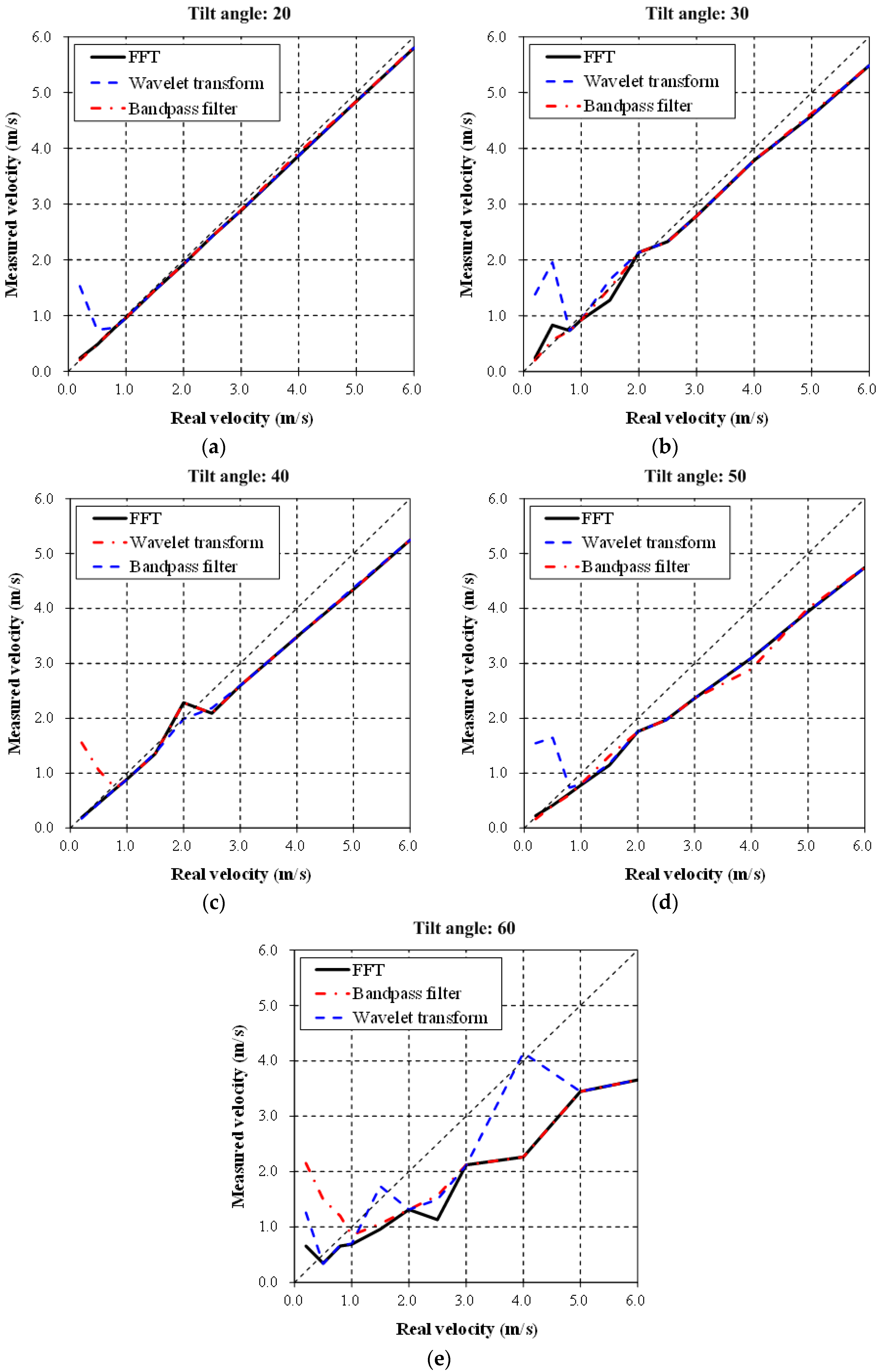
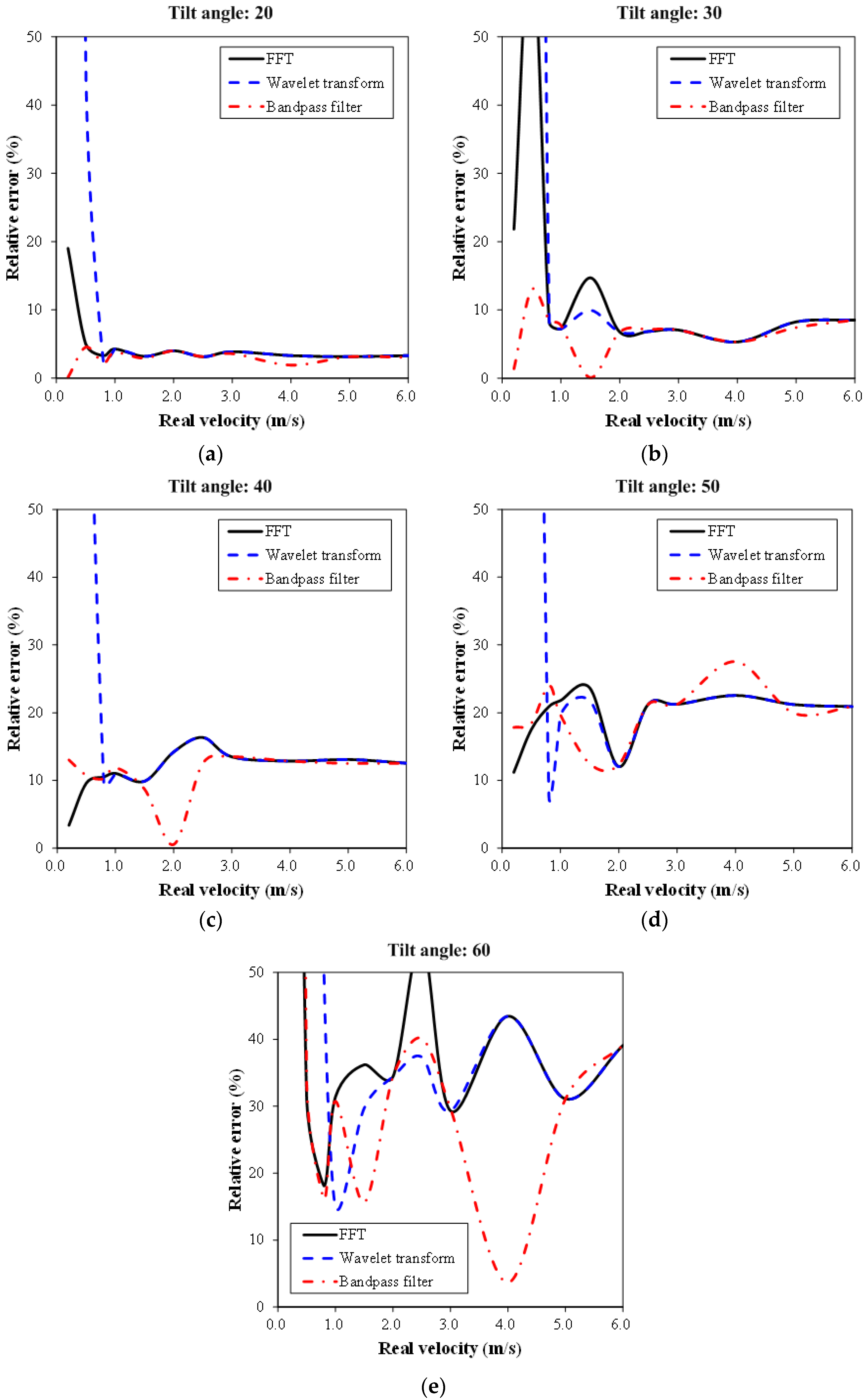
Table 1 and
Table 2, and
Figure 9 and
Figure 10, show the comparison of the identification results and the relative errors under different tilt angles and speeds of the trolley. When the velocity is less than 1.0 m/s (low frequency), the relative error of the wavelet analysis is larger because the selected detail signal is suitable for a high frequency signal, which is unsuitable for a low frequency velocity, in general. When the velocity is greater than 1.0 m/s for the high frequency signal, the results of the wavelet analysis and FFT are similar, possibly because of discarding the approximation signal (low frequency part) because it is negligible in the wavelet signal analysis process. In general, the signal processing of the bandpass filter was more stable and the computed flow velocity had the lowest relative error (as low as 2.84% for a tilt angle of 20 degrees). This is because the proposed bandpass filter could remove the white noise effectively. The analysis results show that all the methods tend to be less accurate as the velocity increases owing to the restrictions in the laboratory (
i.e., the stable movement section in
Figure 4 is 65 m for the measurement). In the 65 m section, when the moving speed of the trolley is higher, fewer original signals could be measured. The length of the measured original signal will affect the analysis results. The optimal range of the tilt angle was between 20 and 40 degrees and the measurement results would be imprecise if it was larger than 40 degrees (the relative error will become higher). This is caused by the limitation of the 10.525-GHz radar wave antennae.


