Automated Method for Monitoring Water Quality Using Landsat Imagery

Abstract

Regular monitoring of water quality is increasingly necessary to keep pace with rapid environmental change and protect human health and well-being. Remote sensing has been suggested as a potential solution for monitoring certain water quality parameters without the need for in situ sampling, but universal methods and tools are lacking. While many studies have developed predictive relationships between remotely sensed surface reflectance and water parameters, these relationships are often unique to a particular geographic region and have little applicability in other areas. In order to remotely monitor water quality, these relationships must be developed on a region by region basis. This paper presents an automated method for processing remotely sensed images from Landsat Thematic Mapper (TM) and Enhanced Thematic Mapper Plus (ETM+) and extracting corrected reflectance measurements around known sample locations to allow rapid development of predictive water quality relationships to improve remote monitoring. Using open Python scripting, this study (1) provides an openly accessible and simple method for processing publicly available remote sensing data; and (2) allows determination of relationships between sampled water quality parameters and reflectance values to ultimately allow predictive monitoring. The method is demonstrated through a case study of the Ozark/Ouchita-Appalachian ecoregion in eastern Oklahoma using data collected for the Beneficial Use Monitoring Program (BUMP).

1. Introduction

The Clean Water Act (CWA) of 1972 [1] was enacted to make the waters of the United States fishable, drinkable, and swimmable in recognition of their vital role for industry, recreation, and food production. As part of this mandate, federal, state, and tribal partners are required to regulate and monitor waterways to ensure compliance. Monitoring public waters can be difficult, though, as field sampling campaigns are labor and time intensive, often requiring additional laboratory costs for sample analysis. In many cases, only a handful of samples are collected and averaged from each water body, which homogenizes any variation in parameters across the lake. Remote sensing offers a potential solution to the obstacles of in situ monitoring since publicly available data are collected at regional scales and temporal resolutions (i.e., repeat collection time) that are much more frequent than field sampling campaigns. Extracting water quality measurements directly from satellite imagery can also allow rapid identification of impaired waters, potentially leading to faster responses by water agencies.

Monitoring water quality through remote sensing involves first determining a reliable relationship between light reflectance (at certain wavelength bands) and water parameters collected in situ. The primary factors influencing the spectral reflectance of water are chlorophyll, dissolved organic matter, and suspended minerals [2,3], which comprise the main components mandated for sampling [4], as well as physical factors such as wind-induced mixing and restratification. Historically, aerial photographs provided the reflectance component to determine these relationships [5], but modern research utilizes satellite imagery. Specifically, studies focus on determining which waveband, or band combinations, correlate with certain water quality parameters such as chlorophyll, total suspended matter, suspended sediment concentration, turbidity, and Secchi disk depth [6,7,8,9,10,11,12,13,14,15,16,17,18,19,20,21].

Some studies have achieved reliable, predictive relationships (R² > 0.8) between reflectance and turbidity, suspended sediments, and Secchi disk depth [10,11,12], thus supporting the further use of remote sensing for water quality monitoring. However, most studies focus on a single geographic region and/or a single water quality parameter. Since relationships between reflectance and water quality will vary across ecoregions, lake taxonomy, seasons, and are impacted by local environmental conditions including weather events [14,22,23], universal predictive models to extract water quality parameters from remote sensing data are difficult to develop [8,12,15,24].

For that reason, these relationships must be developed independently for each region of interest, which can be a hindrance for agencies without expertise in remote sensing or without the time to dedicate to the extensive image processing. The objective of this study is to develop an automated method to extract remotely sensed reflectance values from Landsat imagery based on water sample point locations that can be applied universally provided a database of water sampling parameters, with locations, exists. Subsequently, correlations between sample sampled parameters and reflectance bands can allow development of regional predictive algorithms for monitoring water quality remotely. The method and workflow are demonstrated through a case study of the Ozark/Ouchita-Appalachian ecoregion in eastern Oklahoma using water samples collected for the Beneficial Use Monitoring Program (BUMP).

2. Study Area

Eastern Oklahoma has a range of water issues including high sediment loads and anthropogenic phosphorus, which can cause undesirable algal growth. The Oklahoma Water Resources Board (OWRB) is tasked with monitoring Oklahoma water bodies to ensure compliance with CWA regulations. OWRB collects water quality samples for approximately 25 percent of the lakes in the state in any given year. Due to labor, time, and cost limitations, each lake is sampled, at minimum, once every five years. This sampling frequency allows detection of long-term trends and basic impairment but is insufficient to monitor short-term shifts such as influx from storms or seasonal algal blooms, which can be highly localized and temporally brief but highly destructive. Additionally, on average, only four samples are collected in each lake during each sampling event, which limits the ability to detect localized issues.

The Ozark/Ouachita-Appalachian Forest ecoregion (OOAF) is located in eastern Oklahoma (Figure 1). The Neosho River, with sources in Kansas, Missouri, and Arkansas, is the longest water system. Important uses of the watersheds in this region include the freshwater supply for Tulsa, Oklahoma (a metropolitan area of about 1 million people), the largest recreational lake in Oklahoma (Lake Eufaula), and tourism along the Illinois River, which is an Oklahoma Scenic River. Since the ecoregion boundary bisects many of the major lakes in the region, the boundary was modified slightly to encompass these water bodies (Figure 1–inset).

Common water impairments in this region include high total phosphorus and low dissolved oxygen due to consumption by algae [4], with some waters experiencing eutrophication. The area is also of political interest and the focus of several scientific studies due to intensive agricultural activities upstream (i.e., poultry farming) [1,4,5,7,8,9,25,26,27]. Recently, the state of Oklahoma sued the EPA and several Arkansas municipalities in defense of its waters, resulting in the establishment of separate Total Maximum Daily Loads (TMDL) on phosphorus for Oklahoma’s designated Scenic Waterways, which are enforceable at the Oklahoma border [28]. The ability to remotely monitor these waters frequently is critical to enforce these standards.

3. Material and Methods

3.1. Datasets

To utilize the automated method described below, users need the following datasets: (1) a database of water quality samples collected in situ after 1 March, 1984 (Landsat 5 Thematic Mapper ™ launch date); (2) Landsat TM or Enhanced Thematic Mapper Plus (ETM+) images downloaded from the United States Geological Survey (USGS) Earth Explorer Global Visualization Viewer (GloVis) site [29], acquired within a specified time window of sample collection (e.g., one day), and covering the lake(s) of interest; (3) lake boundary shapefiles, which can be downloaded from the National Map [30]. These datasets are described in detail for the case study below.

3.1.1. BUMP Water Quality Samples

The BUMP database contains water samples from 1998 to present for 130 lakes in Oklahoma (40 in the OOAF ecoregion), but the case study is limited to the 10-year period between October 2003 and October 2012. Sampled water quality parameters include nitrogen, phosphorus, turbidity, dissolved metals, salinity, chlorophyll, and water depth. Data are collected by the OWRB using a combination of digital mensuration tools, field measurements, and lab analysis [31]. While nitrogen and phosphorus are becoming increasingly important for water quality monitoring, chlorophyll is often used as a proxy for those nutrients [32,33], and this is the case with the BUMP data. We focus specifically on chlorophyll-α (hereafter, chlorophyll) and turbidity, which is a proxy for suspended sediment, since these parameters are widely noted to be of concern in both the study area and the literature. It should be noted though that the methodology described below can be applied to any water quality parameters provided sufficient data exist.

OWRB measures chlorophyll (µg/L) by collecting water samples in a flask at each sample site and sending samples to a lab for extraction. Turbidity, which is a composite of suspended sediments, chlorophyll, dissolved organic matter, and air bubbles, is measured using a digital turbidity meter (Hach, Loveland, CO, USA) that calculates the amount of light passing through the water column. Perfectly clear water (i.e., no turbidity) will produce a reading of 0 NTU (Nephelometric Turbidity Units), whereas water with high amounts of sediment and other matter will produce turbidity values as high as 1600 NTU.

As with many sampling programs, BUMP sampling frequencies and configurations are not systematic. Larger lakes typically comprise more sampling sites and are sampled more frequently than smaller water bodies. Additionally, the entire suite of sampling parameters is not always collected for each lake depending on time and cost constraints. Despite these limitations, the BUMP database contains several thousand entries (226 sample locations for the 40 lakes in the ecoregion sampled multiple times over the 10-year study period), which is sufficient for building statistical relationships. The processing methodology and associated Python code (discussed in detail below) are tailored specifically for the BUMP shapefile data format [28], but users can adjust the code to ingest other geospatial formats.

3.1.2. Remote Sensing Imagery

Landsat is widely-used for water quality studies and was therefore selected as the foundation for this method. The processing methodology described here is applicable for Landsat 5 TM and Landsat 7 ETM+ imagery. Additionally, users can utilize Landsat 8 Operational Land Imager (OLI) and Thermal Infrared Sensor (TIRS) imagery by modifying the code to bypass the radiometric correction steps. Since the spectral bands of Landsat 8 (OLI) are very similar to TM and ETM+, it is also possible to develop statistical relationships using TM and ETM+ imagery and then apply those relationships to current and future OLI data collections. Since the sampling methodology utilizes small, 3 × 3 windows placed around sample points (discussed below), it is possible to employ ETM+ images collected after the scan line corrector failed (SLC-off) in 2003 as the analysis will utilize any and all viable pixels in the window.

Users must download scenes prior to running analyses from the USGS Earth Explorer GloVis site [29]. When selecting images for water quality correlation studies, research suggests that imagery should be acquired within one day of an in situ collection event [11,13]. This conservative window limits the availability of cloud-free, Landsat images, and for certain stable parameters (e.g., Secchi disk depth), longer windows up to seven days may be acceptable [13]. However, local environmental conditions, such as wind forces that may cause resuspension of material, may warrant much shorter viable windows. Therefore, the determination of appropriate time window for each study is left to the discretion of the user. For our case study, we elected to only include images collected within one day of (before or after) an in situ sampling event due to the highly variable weather patterns in Oklahoma. When selecting imagery for download, users must also determine an acceptable cloud cover percentage. We included all images with less than 100 percent cloud cover because small lakes may not be occluded by clouds, even in cloudy images, and the atmospheric correction steps will detect and mask out cloud pixels. However, choosing a more stringent cloud threshold can reduce processing time and potentially eliminate unnecessary processing for lakes occluded by clouds. Lastly, since all bands including thermal, are needed for image preprocessing, we retain all bands for analysis. Most water quality studies utilize only the visible and near infrared (NIR) portions of the electromagnetic spectrum, so users may elect specific bands to analyze after processing has concluded.

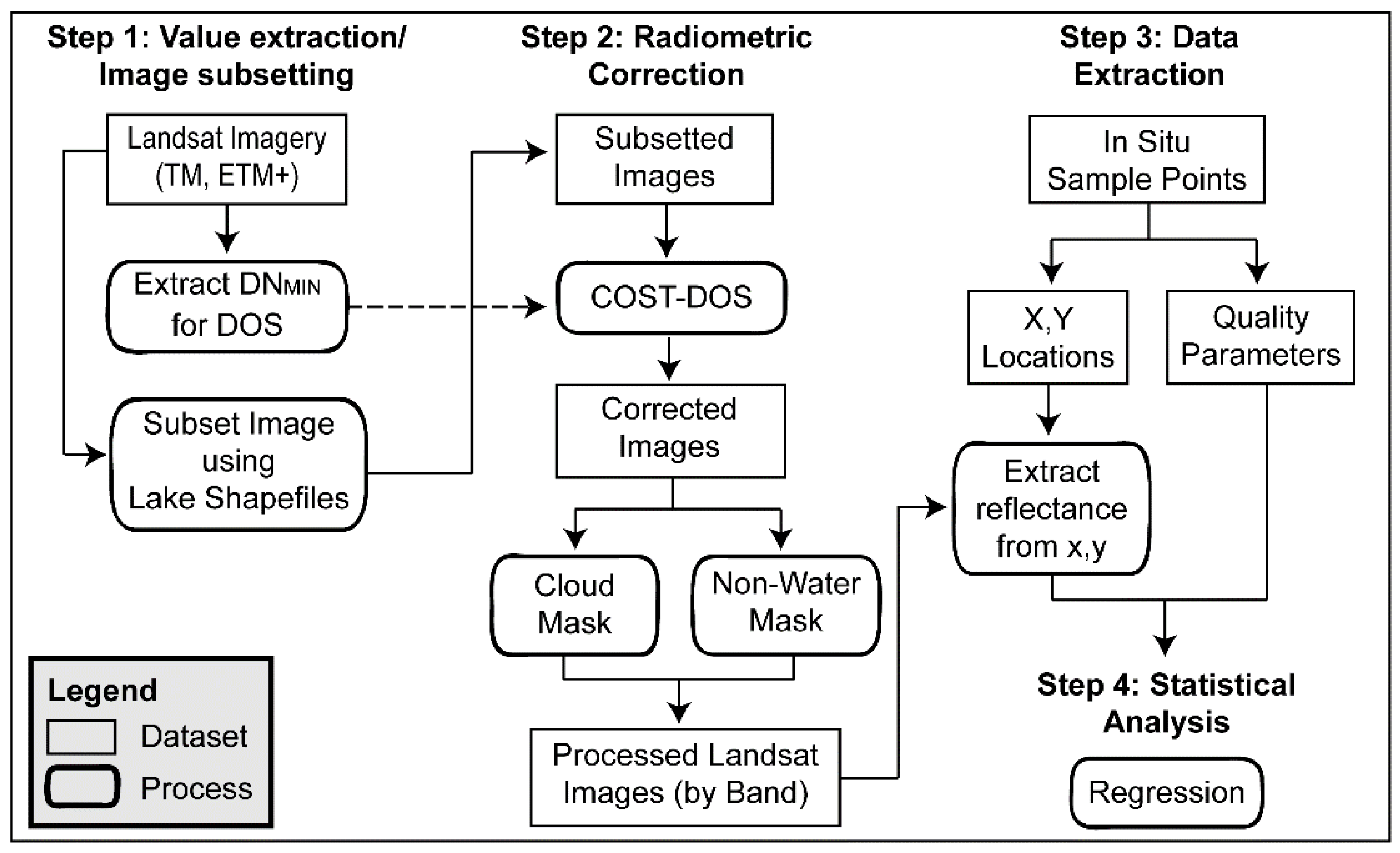
3.2. Image Processing Methodology

The automated image processing method is built in the open Python scripting language [34]. Image manipulation is performed in Python using ArcMap (Esri, Redlands, CA, USA) [35] via the arcpy module. Arcpy is a version of Python built by Esri (Redlands, CA, USA) that can access ArcMap functions and includes the NumPy package. The Arcpy module is utilized to control ArcMap from outside the program, thus allowing ArcMap functions to be called in the same manner Python functions are called. These script tools were developed in Python specifically to allow easy distribution, access, and use by others [36]. However, the use of Arcpy requires an Esri ArcMap™ license with the Spatial Analyst extension. The Python script presented below is available in the Supplementary materials. Python software can be downloaded from www.python.org.

The processing methodology (Figure 2) includes four stages: (1) minimum value extraction and image subsetting; (2) radiometric correction including water and cloud masks; (3) extraction and averaging of spectral reflectance values in sample point windows; and (4) statistical analysis (i.e., regression). The first three stages are automated through the Python script. Once reflectance values have been extracted, statistical correlations and regressions can be built by the user to determine relationships between water quality parameters and surface reflectance. It should be noted that Landsat surface reflectance products can be substituted for raw imagery when available, which eliminates the need to perform Step 2. This step can easily be skipped in the processing code by toggling it off.

3.2.1. Step 1: Value Extraction and Image Subsetting

Once images are downloaded and unzipped by the user, the Python script extracts the lowest pixel digital number (DN_min) occurring throughout the image at least 100 times to use later on during radiometric correction. This value needs only be assessed once for each scene, and is saved so that lakes and associated sampling events sourced from the same Landsat scene will utilize the same DN_min value. Once the DN_min value has been extracted, images are clipped to the rectangular extent of the lake. Since water levels fluctuate, and complex lake boundary vectors are computationally expensive for clipping, the script reprocesses lake outlines to rectangles bounding the outer extent of the shoreline, which expedites the process. Non-water areas within the rectangle are masked out on a per image basis in Step 2.

3.2.2. Step 2: Radiometric and Atmospheric Correction

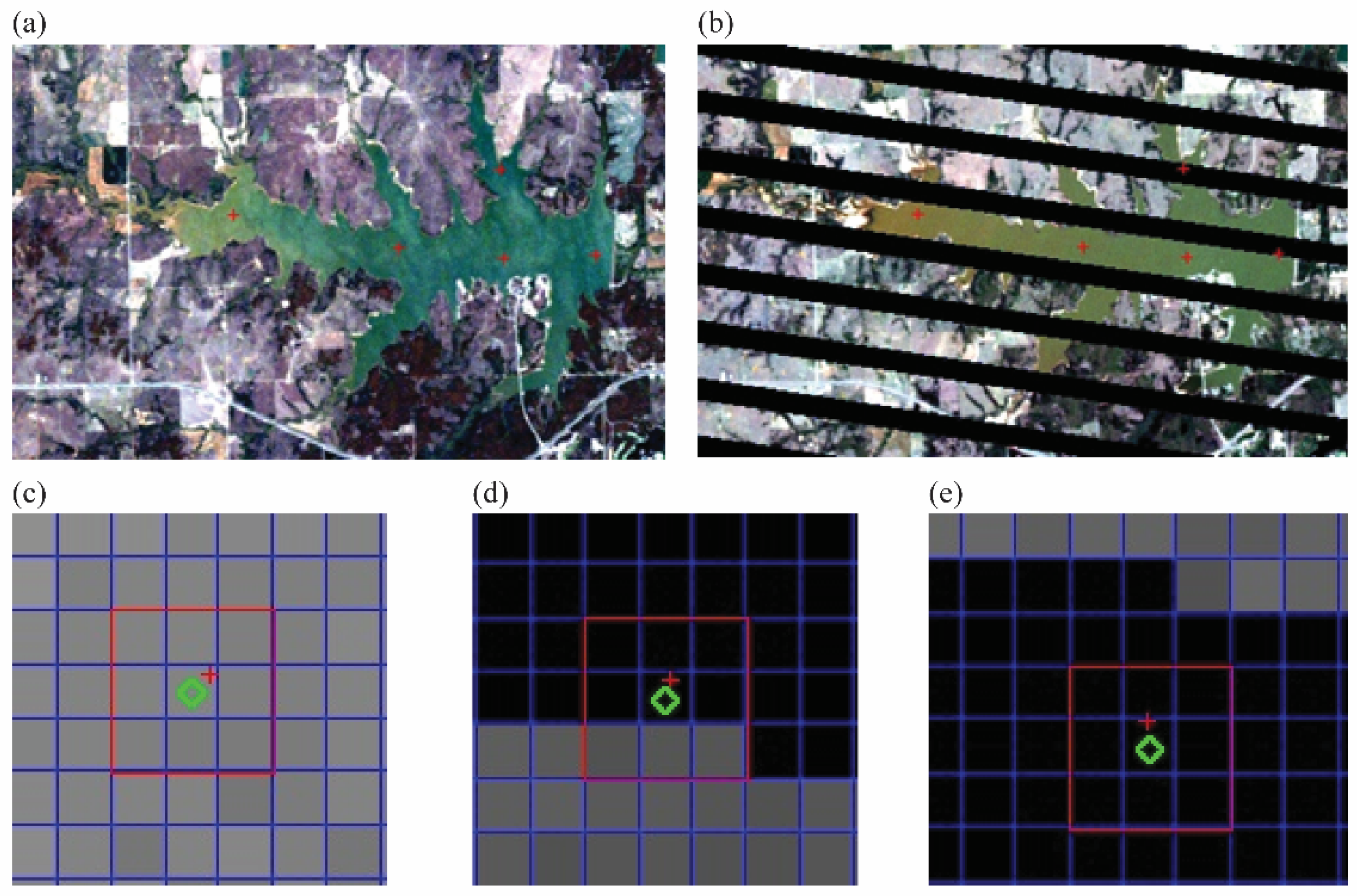
COST-DOS, or cosine of the solar zenith angle correction dark object subtraction, is a radiometric correction method for mitigating atmospheric effects recorded by satellite remote sensing instruments [37]. COST-DOS correction can account for scattering, absorption, and refraction of light from atmospheric particles such as water vapor and particulate matter. This method is built from two parts: dark object subtraction (DOS) accounts for additive radiometric error through histogram shifting, while the cosine of solar zenith (COST) addresses multiplicative error by accounting for the variation in sun angles throughout the year [37]. COST-DOS atmospheric correction does not require field radiometric measurements, which makes it ideal for correcting historical imagery. However, the method does require a seasonally invariant dark object, such as a clear lake or manmade structure, to be present within the image, so researchers should take care to ensure this assumption is satisfied prior to implementing the method. The inputs for COST-DOS include DN_min, which was collected in Step 1 from the complete Landsat scene before subsetting. Additional inputs are the solar zenith angle and distance between the earth and sun, which are automatically obtained from the image header file (metadata), and the scene’s pixel values, which are recalculated to the top of atmosphere (TOA) values originally captured by the sensor, using Equation (1) [38]:

$$L_{\lambda }=M\rho *QCAL+A\rho$$

(1)

where L_λ is TOA reflectance, QCAL are the quantized calibrated pixel values in DN, Mρ is the multiplicative rescaling factor, and Aρ is the additive scaling factor. Equation (1) converts DN to TOA reflectance but does not account for atmospheric effects. COST-DOS calculates rescaling factors from the minimum and maximum calibration values and includes DOS correction and sun angle correction in this process. The generic and expanded forms of this equation are described in Equations (2)–(4):

$$L_{haze}=H{L}_{min}-L_{1\text{\%}}$$

(2)

where:

$$H{L}_{min}=L_{min}+D{N}_{min}\frac{\left(L_{max}-L_{min}\right)}{\left(QCA{L}_{max}-QCA{L}_{min}\right)}$$

(3)

$$L_{1\text{\%}}=\left(0.01+ESU{N}_{\lambda }*\cos {\left({\varnothing }_s\pi /180\right)}^2\right)/\left(d^2\pi \right)$$

(4)

Most of the input data for Equations (2)–(4) are contained in the Landsat metadata file, which accompanies the image when downloaded from the USGS site [29]. $L_{max}$ and $L_{min}$ are maximum and minimum spectral radiances values scaled to$QCA{L}_{max}$ and $QCA{L}_{min}$ by band. The difference between $QCA{L}_{max}$ and $QCA{L}_{min}$ for 8-bit imagery is 254 and has been this value [(255–1)] since a recalibration in 2004. $D{N}_{min}$ is the lowest pixel value (originally in DN but converted to TOA reflectance in $H{L}_{min}$) with at least a count of 100 in the raw scene. $ESU{N}_{\lambda }$ is the solar spectral irradiance at TOA. These are known values published for each satellite [39,40]. ${\varnothing }_s$ is the solar zenith angle in degrees, which is calculated from the sun elevation included in the metadata minus 90⁰. Finally, the distance between the Earth and sun, $d$, can be determined using the Julian acquisition date contained within the Landsat file name. The outcome, $L_{haze}$, is the rescaled and corrected $D{N}_{min}$ value, which is used to correct the rescaled image values during their correction process (Equation (5)):

$$P_{\lambda }=\frac{\pi \left(L_{\lambda }-L_{haze}\right)d^2}{ESU{N}_{\lambda }\text{cos}\left(\pi /180{\theta }_s\right)}$$

(5)

The atmospherically corrected reflectance ($P_{\lambda }$) is the final outcome using the TOA reflectance ($L_{\lambda }$) minus the rescaled and corrected $D{N}_{min}$ value, correcting for variations in the angle, distance, and brightness of the sun throughout the year.

The thermal band is eventually used to produce a cloud cover detection algorithm and ultimately mask out any cloud areas so they do not influence results (see below). Radiometric correction of the thermal band involves first converting values to spectral radiance using Equation (1) and then converting spectral radiance to surface temperature using Equation (6). This conversion requires two calibration constants: $K_1$ and $K_2$ [40]. The output of Equation (6) is temperature in kelvin for every pixel in the image:

$$T=\frac{K_2}{\text{ln}\left(\frac{K_1}{L\lambda }+1\right)}$$

(6)

3.3. Cloud Mask

A cloud cover map is not available for each Landsat scene, but the process used to compute cloud cover by USGS is mimicked in this script to generate a cloud cover map for the purpose of excluding cloud pixels from data extraction. The process, detailed by Irish [41], consists of a two-pass process using thresholds and indices to check for dense clouds and filter out sand and snow, both of which exhibit similarities to cloud reflectance. Cirrus clouds are not detected by this method due to their lack of a strong thermal response [41].

The first pass comprises eight filters, which progressively differentiate pixels as either “cloud” or “not cloud”. Pixels identified as “not cloud: that can be positively labeled as snow or sand are noted for later use. Pixels classified as ambiguous proceed to the second pass where they are reevaluated using basic statistics computed from pixels detected as ‘clouds’ during the first pass. If an excess of brightly illuminated desert pixels are detected in the first pass, the second pass is not executed. If snow is present in the scene, cloud pixels are divided into warm and cold classes with the statistics of each used to evaluate ambiguous pixels during the second pass; otherwise, the entire cloud class is utilized. The cloud statistics set minimum and maximum classification thresholds for reevaluating ambiguous pixels to determine if they are cloud or not cloud. The final result of this process is a binary raster where pixels coded 1 are cloud free and can be extracted for analysis.

3.4. Water Mask

The final radiometric/atmospheric correction step is to mask out pixels that do not contain water. Due to seasonal fluctuations in water level and longer-term impacts such as drought, sample locations may not always be located over water. It is necessary to exclude these pixels so they do not influence results. The Normalized Difference Water Index (NDWI) [42] was designed to detect water content of leaves, and has been modified to better highlight water information in Landsat bands [43] (Equation (7)). The result of the modified NDWI (MNDWI) is a binary mask with values of 1 for pixels containing water. Pixels with values of 1 are extracted for analysis:

$$MNDWI=\frac{Green-SWIR1}{Green+SWIR1}$$

(7)

3.4.1. Step 3: Data Extraction

To extract reflectance data for analysis, the script selects the pixel containing the x, y location of the in situ sample point and identifies a 3 × 3 pixel window centered on that point. The selection of a nine-pixel window is based on the assumption that water is heterogeneous and often in flux due to seasonal, solar, and meteorological factors, so a larger window will capture some of that variance. Additionally, neither GPS points nor water samples will be collected in precisely the same position every sampling event given they are typically collected from a vessel in moving water. More importantly, Kloiber, et al. [13] investigated various pixel window sizes, up to 25 × 25, for water quality analysis and found that windows larger than 3 × 3 pixels were not statistically advantageous. In this study, we utilize a 3 × 3 pixel window, but the window size is customizable. The script extracts viable reflectance values from within the 3 × 3 window based on the cloud and water masks and averages those reflectance values to produce mean values for each band for each respective sample point. Since a sample window may have less than nine viable pixels (due to clouds, non-water, or SLC-off voids: Figure 3), the script also generates a ratio of the number of viable pixels used to compute each sample, by band, so users can independently determine an acceptable minimum value threshold for each individual study by sorting results based on this field and eliminating any windows with a lower completion ratio than desired.

3.4.2. Step 4: Statistical Analysis

We perform statistical analyses here to demonstrate how the aforementioned data processing methodology can be used to develop relationships between reflectance and in situ sample data to allow prediction of water quality remotely. However, it is important to note that these relationships will change based on the geographic location, ecoregion, lake type, and season in which sampling occurs, so relationships must be calibrated for the specific region under investigation. It is also important to note that, due to the variabilities and uncertainties of water quality parameters, developing robust prediction algorithms may not be possible in all ecoregions.

We computed mean reflectance values for each sample point and correlate various band and band combinations with turbidity and chlorophyll. Since each sample location was visited multiple times across the 10-year study period, we treat each event as an independent sample since the water sampled was undoubtedly different despite coming from a relatively similar position in the lake. We performed regression analyses using the Statistical Package for the Social Sciences (SPSS; IBM, Armonk, NY, USA) [44], but users may opt for any statistical software program since this step must be performed after the automated processing script has finished.

We first performed basic data explorations (e.g., summary statistics, normality tests, etc.) to determine possible candidate models for predicting water quality (chlorophyll/turbidity) from reflectance. Transformed and raw reflectances were then correlated with water quality parameters by individual band, band pairs, and other band combinations using Pearson’s r. We tested all possible combinations of bands for band ratios. Since seasonality affects water quality in this region, we also examined correlations by season: winter (Jan–Mar), spring (Apr–Jun), summer (July–Sept), and fall (Oct–Dec). Correlations from each season with significant and meaningful r values were tested with linear bivariate regression.

4. Results and Discussion

4.1. Processing Methodology and Code

The processing code is available in the Supplementary electronic materials. Image processing was performed on an Intel i5 processor (Santa Clara, CA, USA) and took approximately 35 min to process a large lake with 14 images with 34 sample points. The design of this tool around the OWRB’s water quality database and lake shapefiles allows rapid reapplication of this methodology across Oklahoma, and with minor changes, it can easily be applied to other water sample databases. While the code was written specifically for Landsat 5 and 7, it can integrate Landsat 8 with minor adjustments. In the development of these scripts, portions of the code were adopted from Gómez-Dans [45] and Kochaver [46]. These scripts provided insight that expedited the development of this tool, and our intent is that public release of this script will aid in future water research.

4.2. Case Study Results

Over the ten-year study period, 130 Landsat scenes coincided within one day of a BUMP sampling event. After verifying that each sample window contained lake surface reflectance and was complete for all bands, we extracted 9369 sample locations, which gave us 347 paired pixel extracts and BUMP samples (n = 347). We elected to use all sample windows, even those with less than 100 percent viability (<9 pixels with reflectance values). For the most part, data presented bimodal distributions, which is typical for lakes with the two modes corresponding to deep water and shallow water. Chlorophyll and turbidity, the two variables examined, both exhibited a logarithmic distribution, so the data were natural log transformed to improve normality. Correlations for both the raw and log-transformed parameters are presented.

Significant results (α < 0.01) for chlorophyll and lnChlorophyll (

Table 1. Significant (α < 0.01) relationships between reflectance bands/band combinations and chlorophyll, by season.

Significant Results (n)	Band/Band Combinations	Pearson’s r Values
All data (347)
Chlorophyll	SWIR2/NIR	−0.154
lnChlorophyll	SWIR2/NIR	−0.155
Winter (74)
Chlorophyll	SWIR1/SWIR2 Blue/SWIR2 SWIR2/Green	0.498 0.273 0.238
lnChlorophyll	SWIR1/SWIR2	0.379
Spring (94)
Chlorophyll	None	N/A
lnChlorophyll	NIR/SWIR1 Green/SWIR1 Red/SWIR1 Green/SWIR2 NIR/SWIR2	−0.356 −0.346 −0.319 −0.306 −0.303
Summer (99)
Chlorophyll	None	N/A
lnChlorophyll	None	N/A
Fall (80)
Chlorophyll	None	N/A
lnChlorophyll	None	N/A

) show positive correlations between reflectance and chlorophyll during winter, with a negative relationship during spring. While r values are not particularly high, all reported values are significant. Interestingly, all significant band combinations for chlorophyll included at least one of the short wave infrared bands (SWIR), yet most water quality studies to this point have not included SWIR bands. These results suggest there may be a relationship between SWIR reflection and algae/plant production, which deserves further investigation. It is possible that ratios between either chlorophyll absorption bands (red and blue) or chlorophyll reflectance bands (green and NIR) with either of the two SWIR bands may accentuate the portion of the spectrum affected by chlorophyll, thereby making estimated values more readily correlated with actual sample values. Chlorophyll was not significantly correlated with any bands or band combinations during summer, which is surprising given the propensity for algal formations in the study region. However, algae blooms can be temporally brief, and may not have aligned with the eight to 16-day temporal resolution of the images.

Significant results (α < 0.01) for turbidity and lnTurbidity (

Table 2. Significant (α < 0.01) relationships between reflectance bands/band combinations and turbidity, by season.

Significant Results (n) *	Band/Band Combinations	Pearson’s r Values
All data (347)
Turbidity	None	N/A
lnTurbidity	SWIR1 SWIR2 Red/SWIR1 NIR/SWIR1 Red/SWIR2	−0.142 −0.145 0.421 0.409 0.431
Winter (74)
Turbidity	Green/SWIR1 Green/SWIR2	0.455 0.523
lnTurbidity	Red/SWIR1 NIR/SWIR1 Red/SWIR2	0.510 0.503 0.470
Spring (94)
Turbidity	None	N/A
lnTurbidity	Green/Red Blue/Red SWIR2/NIR SWIR2/Blue	−0.464 -0.422 0.329 0.273
Summer (99)
Turbidity *	Red/Green	0.359
Turbidity *	Red/SWIR1 Red/SWIR2 NIR/SWIR1 NIR/SWIR2	0.411 0.354 0.43 0.362
lnTurbidity*	Red/SWIR1 NIR/SWIR1 NIR/SWIR2	0.496 0.494 0.422
lnTurbidity*	Red/SWIR2 SWIR2/NIR	0.427 −0.417
Fall (80)
Turbidity	Green/Red	−0.383
Turbidity	Red/B5	0.281
Turbidity	NIR/SWIR1	0.335
Turbidity	NIR/SWIR2	0.303
lnTurbidity * lnTurbidity * lnTurbidity * lnTurbidity * lnTurbidity *	Green NIR SWIR1 SWIR2 NIR/SWIR1	−0.442 −0.443 −0.464 −0.449 0.461

Note: * Only top five correlations, in terms of r value, shown.

) show individual band correlations were strongest for SWIR1 and log-transformed SWIR2 for lnTurbidity. The addition of red and NIR bands to ratios with the SWIR bands improved r values. In winter, several band combinations containing a SWIR band were significant. A linear regression composed of Red/SWIR1 and Blue/SWIR1 produced a moderately high r² value (0.648) suggesting that the SWIR1 bands in combination with the chlorophyll absorption bands (red and blue), may hold value for detecting turbidity. This combination is not surprising since turbidity is a composite of suspended sediments, chlorophyll, and other dissolved organic matter; SWIR bands are specifically designed to detect reflectance from minerals (i.e., sediments), and the blue and red bands are suitable for detecting chlorophyll. Previous research has indicated possible relationships between turbidity and red reflectance [13] and NIR reflectance [11], but, to our knowledge, this is the first study noting strong relationships between turbidity and SWIR bands.

In summer, there were eight significant Turbidity relationships ranging from 0.252 to 0.43, and lnTurbidity had 14 significant correlations ranging from 0.277 to 0.496. Significant band correlations included various combinations of the Red, NIR, and SWIR bands. Lastly, during fall, lnTurbidity was significantly correlated with all six individual bands, their natural log transformations, and ten independent band ratios. Correlations varied from −0.292 to 0.461. Interestingly, all band ratios included an infrared band: NIR, SWIR1, or SWIR2. Controlling for excessive influence of the green band in a stepwise regression of the significantly correlated variables, r² = 0.555 and included the NIR, lnRed, and lnBlue bands. However, multicollinearity was present between the lnRed and lnBlue bands.

Linear regressions were run for the best performing samples to determine predictive relationships from multiple variables. lnTurbidity showed the best significant (α < 0.01) regression relationship (r² = 0.521) in winter using several band ratios:

$$\text{ln}Turbidity=6.7+0.62\frac{Red}{NIR}-0.882\frac{NIR}{Blue}-3.22\frac{Green}{Blue}$$

(8)

While our case study was primarily intended to demonstrate how the automated processing methodology can be used to develop relationships between surface reflectance and water quality samples, it is useful to compare our results with prior studies that have used Landsat imagery for water quality prediction in an effort to develop globally applicable algorithms. For example, Hicks et al. [11] generated Pearson correlation coefficients between −0.46 and 0.96 for turbidity for lakes in New Zealand using Landsat 7. They reported strongest relationships (>0.90) for single bands Blue, Red, and NIR. We also uncovered a significant relationship between lnTurbidity and the single NIR band in fall (Table 2) but did not find any strong relationships for the individual Blue and Red bands. Similarly, Allen et al. [6] generated correlation coefficients as high as 0.944 for chlorophyll using the band ratio Blue/Red from Landsat 7, also for a lake in New Zealand, where conditions vary extensively from the study area examined here. Interestingly, neither study incorporated the SWIR bands, which were found in this study to be significant, both as individual predictors and as components of band ratios. Every significant predictor ratio in our study for chlorophyll included a SWIR band, which suggests that regional environmental differences may warrant use of SWIR bands. Jiazhu [12] produced more moderate correlation coefficients, similar to the values observed in this study, with absolute values ranging from 0.018 to 0.826 for Taihu Lake in China, which experiences high degrees of eutrophication and pollution. That study, which used Landsat TM imagery, also found seasonal differences between prediction strength, which is in line with the findings from this study. Specifically, we found similar moderate regression relationships for turbidity during winter, when lake water quality in Oklahoma is most stable. Together, these results suggest that reflectance relationships, particularly for eutrophic lakes, may be season-dependent.

In general, our results were likely not as strong as prior studies due to the unique lake morphology and water composition in eastern Oklahoma, which is vastly different from the oligotrophic lakes studied by Allan, et al. [6] and Hicks, et al. [11]. However, the main contribution of this research is that the automated processing methodology allowed us to process and analyze hundreds of samples across all seasons while many prior studies have relied on a much smaller number of samples collected during one or a few sampling campaigns. Weak correlations, particularly in spring and summer, may also be due to the lake turnover effect, when the equalization of the thermal gradient in the lake induces mixing of surface and bottom waters, making remote monitoring difficult due to instability. Further analysis of the specific boundaries when strong relationships are found may help improve prediction capabilities by providing researchers with bounded time periods (according to region), during which remote monitoring is feasible. We implemented a conservative, one-day window surrounding BUMP sample events, but increasing that window would yield more images and ultimately increase the number of sample pairs. Since physical parameters such as turbidity stabilize during low influx times of the year [16], this is a plausible alternative. Any reduced correlation strength for additional observations would be offset by the increase in the number of observations [13].

5. Conclusions

This study developed an automated method for processing remotely sensed Landsat images and extracting reflectance measurements from sample location windows. These reflectance values can, in turn, be used to develop predictive water quality monitoring relationships. The processing methodology can be adjusted by the user based on image window preference (i.e., time before and after sampling event) and sample window (i.e., number of pixels surrounding sample GPS point). We tested the method on a set of lakes in eastern Oklahoma and found that reflectance in the SWIR was significantly correlated with both chlorophyll and turbidity through ratios with other bands. These relationships were particularly strong in winter when lake water is stabilized. It is hoped that the methodology and automated script made available in this study can be used by others to develop similar relationships for water quality parameters across geographic regions.

References

1. EPA. Summary of the Clean Water Act. Available online: http://www2.epa.gov/laws-regulations/summary-clean-water-act (accessed on 12 June 2016).
2. Bukata, R.P. Optical Properties and Remote Sensing of Inland and Coastal Waters; CRC Press: Boca Raton, FL, USA, 1995. [Google Scholar]
3. Jensen, J.R. Remote Sensing of the Environment: An Earth Resource Perspective; Pearson Prentice Hall: Upper Saddle River, NJ, USA, 2007. [Google Scholar]
4. EPA. TMDL Development for Lakes Eucha and Spavinaw in Oklahoma. Available online: http://www.epa.gov/waters/tmdldocs/2Eucha_Spavinaw_TMDL_TP_%20Apr_10.pdf (accessed on 12 June 2016).
5. Goldman, C.R.; Richards, R.C.; Paerl, H.W.; Wrigley, R.C.; Oberbeck, V.R.; Quaide, W.L. Limnological studies and remote sensing of the Upper Truckee River sediment plume in Lake Tahoe, California-Nevada. Remote Sens. Environ. 1974, 3, 49–67. [Google Scholar] [CrossRef]
6. Allan, M.G.; Hamilton, D.P.; Hicks, B.J.; Brabyn, L. Landsat remote sensing of chlorophyll a concentrations in central North Island lakes of New Zealand. Int. J. Remote Sens. 2011, 32, 2037–2055. [Google Scholar] [CrossRef]
7. Carpenter, S.M.; Carpenter, D.J. Modeling inland water quality using Landsat data. Remote Sens. Environ. 1983, 13, 345–352. [Google Scholar] [CrossRef]
8. Dekker, A.G.; Vos, R.J.; Peters, S.W.M. Analytical algorithms for lake water TSM estimation for retrospective analyses of TM and SPOT sensor data. Int. J. Remote Sens. 2002, 23, 15–35. [Google Scholar] [CrossRef]
9. Guneroglu, A.; Karsli, F.; Dihkan, M. Automatic detection of coastal plumes using Landsat TM/ETM+ images. Int. J. Remote Sens. 2013, 34, 4702–4714. [Google Scholar] [CrossRef]
10. Harrington, J.A.; Schiebe, F.R.; Nix, J.F. Remote sensing of Lake Chicot, Arkansas: Monitoring suspended sediments, turbidity, and Secchi depth with Landsat MSS data. Remote Sens. Environ. 1992, 39, 15–27. [Google Scholar] [CrossRef]
11. Hicks, B.; Stichbury, G.; Brabyn, L.; Allan, M.; Ashraf, S. Hindcasting water clarity from Landsat satellite images of unmonitored shallow lakes in the Waikato region, New Zealand. Environ. Monit. Assess. 2013, 185, 7245–7261. [Google Scholar] [CrossRef] [PubMed]
12. Jiazhu, G.J.W.Y.H. A model for the retrieval of suspended sediment concentrations in Taihu Lake from TM images. J. Geogr. Sci. 2006, 16, 458–464. [Google Scholar]
13. Kloiber, S.M.; Brezonik, P.L.; Bauer, M.E. Application of Landsat imagery to regional-scale assessments of lake clarity. Water Res. 2002, 36, 4330–4340. [Google Scholar] [CrossRef]
14. McCullough, I.M.; Loftin, C.S.; Sader, S.A. Combining lake and watershed characteristics with Landsat TM data for remote estimation of regional lake clarity. Remote Sens. Environ. 2012, 123, 109–115. [Google Scholar] [CrossRef]
15. Nas, B.; Ekercin, S.; Karabork, H.; Berktay, A.; Mulla, D.J. An application of Landsat-5TM image data for water quality mapping in Lake Beysehir, Turkey. Water Air Soil Pollut. 2010, 212, 183–197. [Google Scholar] [CrossRef]
16. Olmanson, L.G.; Bauer, M.E.; Brezonik, P.L. A 20-year Landsat water clarity census of Minnesota’s 10,000 lakes. Remote Sens. Environ. 2008, 112, 4086–4097. [Google Scholar] [CrossRef]
17. Onderka, M.; Rodný, M. Can suspended sediment concentrations be estimated from multispectral imagery using only image-derived information? J. Indian Soc. Remote Sens. 2010, 38, 85–97. [Google Scholar] [CrossRef]
18. Ritchie, J.C.; Cooper, C.M.; Schiebe, F.R. The relationship of MSS and TM digital data with suspended sediments, chlorophyll, and temperature in Moon Lake, Mississippi. Remote Sens. Environ. 1990, 33, 137–148. [Google Scholar] [CrossRef]
19. Ritchie, J.C.; Cooper, C.M.; Yongqing, J. Using Landsat multispectral scanner data to estimate suspended sediments in Moon Lake, Mississippi. Remote Sens. Environ. 1987, 23, 65–81. [Google Scholar] [CrossRef]
20. Ritchie, J.C.; Schiebe, F.R.; Cooper, C.M. Landsat digital data for estimating suspended sediment in inland water. Int. Assoc. Hydrol. Sci. Publ. 1989, 151–158. [Google Scholar]
21. Nechad, B.; Ruddick, K.G.; Park, Y. Calibration and validation of a generic multisensor algorithm for mapping of total suspended matter in turbid waters. Remote Sens. Environ. 2010, 114, 854–866. [Google Scholar] [CrossRef]
22. Schalles, J.F.; Rundquist, D.; Schiebe, F. The Influence of Suspended Clays on Phytoplankton Reflectance Signatures and the Remote Estimation of Chlorophyll. In Verh. Int. Ver. Theor. Angew. Limnol./Proc. Int. Assoc. Theor. Appl. Limnol./Trav. Assoc. Int. Limnol. Theor. Appl., Dublin, Ireland, 8–14 August 1998; pp. 3619–3625.
23. Zhou, W.; Wang, S.; Zhou, Y.; Troy, A. Mapping the concentrations of total suspended matter in Lake Tailm, China, using Landsat-5 TM data. Int. J. Remote Sens. 2006, 27, 1177–1191. [Google Scholar] [CrossRef]
24. Kallio, K.; Attila, J.; Harma, P.; Koponen, S.; Pulliainen, J.; Hyytiainen, U.M.; Pyhalahti, T. Landsat ETM+ images in the estimation of seasonal lake water quality in boreal river basins. Environ. Manag. 2008, 42, 511–522. [Google Scholar] [CrossRef] [PubMed]
25. Busteed, P.R.; Storm, D.E.; White, M.J.; Stoodley, S.H. Using SWAT to target critical source sediment and phosphorus areas in the Wister Lake basin, USA. Am. J. Environ. Sci. 2009, 5, 156–163. [Google Scholar] [CrossRef]
26. Haggard, B.; Moore, P.; DeLaune, P. Phosphorus flux from bottom sediments in Lake Eucha, Oklahoma. J. Environ. Qual. 2005, 34, 724–728. [Google Scholar] [CrossRef] [PubMed]
27. Haggard, B.E.; Soerens, T.S. Sediment phosphorus release at a small impoundment on the Illinois River, Arkansas and Oklahoma, USA. Ecol. Eng. 2006, 28, 280–287. [Google Scholar] [CrossRef]
28. Data & Maps: Surface Water. Available online: http://www.owrb.ok.gov/maps/pmg/owrbdata_SW.html (accessed on 12 June 2016).
29. USGS. USGS Global Visualization Viewer. Available online: http://glovis.usgs.gov/ (accessed on 12 June 2016).
30. USGS. The National Map. Available online: http://nationalmap.gov/ (accessed on 12 June 2016).
31. 2012 Oklahoma Lakes Report. Available online: http://www.owrb.ok.gov/quality/monitoring/bump/pdf_bump/archives/2012_LakesBUMPReport.pdf (accessed on 12 June 2016).
32. Chen, J.; Quan, W. Using Landsat/TM imagery to estimate nitrogen and phosphorus concentration in Taihu Lake, China. Sel. Top. Appl. Earth Obs. Remote Sens. 2012, 5, 273–280. [Google Scholar] [CrossRef]
33. Song, K.; Li, L.; Li, S.; Tedesco, L.; Hall, B.; Li, L. Hyperspectral remote sensing of total phosphorus (TP) in three central Indiana water supply reservoirs. Water Air Soil Pollut. 2012, 223, 1481–1502. [Google Scholar] [CrossRef]
34. Python Software Foundation (PSF). Python Language Reference; PSF: Wilmington, DE, USA, 2014. [Google Scholar]
35. Environmental Systems Research Institute (ESRI). Arcgis Desktop; Environmental Systems Research Institute: Redlands, CA, USA, 2014. [Google Scholar]
36. Barrett, C. Monitoring Eastern Oklahoma Lake Water Quality Using Landsat; Frazier, A.E., Comer, J., Zou, C., Eds.; ProQuest Dissertations Publishing: Ann Arbor, MI, USA, 2015. [Google Scholar]
37. Chavez, P.S., Jr. Image-based atmospheric corrections—Revisited and improved. Photogramm. Eng. Remote Sens. 1996, 62, 1025. [Google Scholar]
38. USGS. Landsat 7 Science Data Users Handbook. Available online: http://landsathandbook.gsfc.nasa.gov/data_prod/prog_sect11_3.html (accessed on 12 June 2016).
39. Chander, G.; Markham, B. Revised Landsat-5 TM radiometric calibration procedures and postcalibration dynamic ranges. Geosci. Remote Sens. 2003, 41, 2674–2677. [Google Scholar] [CrossRef]
40. USGS. ACCA Parameters. Available online: http://landsathandbook.gsfc.nasa.gov/cpf/prog_sect9_2.html#section9.2.4 (accessed on 12 June 2016).
41. Irish, R.R. Landsat 7 automatic cloud cover assessment. In Proceedings of the AeroSense 2000, Orlando, FL, USA, 24–28 April 2000; pp. 348–355.
42. Gao, B.C. NDWI-A normalized difference water index for remote sensing of vegetation liquid water from space. Remote Sens. Environ. 1996, 58, 257–266. [Google Scholar] [CrossRef]
43. Xu, H. Modification of normalised difference water index (NDWI) to enhance open water features in remotely sensed imagery. Int. J. Remote Sens. 2006, 27, 3025–3033. [Google Scholar] [CrossRef]
44. International Business Machines Corporation (IBM). IBM spss Statistics; International Business Machines Corporation: Armonk, NY, USA, 2014. [Google Scholar]
45. Gómez-Dans, J. Dn_2_rad.Py. Available online: https://gist.github.com/jgomezdans/5488682 (accessed on 12 June 2016).
46. Kochaver, S. Reflectance.Py. Available online: https://github.com/skochaver/reflectance-tools (accessed on 12 June 2016).
Figure 1. Study area showing modified ecoregion boundary.
Water 08 00257 g001
Figure 2. Methods flowchart.
Water 08 00257 g002
Figure 3. Sampling points (red crosses) overlain on (a) a normal image; (b) an image with scan line corrector off (SLC-off) voids, Bottom images show; (c) a fully intact nine-pixel sample window; (d) a partially occluded sample window; and (e) a fully occluded sampling window.
Water 08 00257 g003