Efficiency of a Horizontal Sub-Surface Flow Constructed Wetland Treatment System in an Arid Area

Abstract

The main objective of this study was to evaluate the performance and treatment efficiency of the Horizontal Sub-Surface Flow Constructed Wetland treatment system (HSF-CW) in an arid climate. Seventeen sub-surface, horizontal-flow HSF-CW units have been operated for approximately three years to improve the quality of partially-treated municipal wastewater. The studied design parameters included two sizes of volcanic tuff media (i.e., fine or coarse), two different bed dimensions (i.e., long and short), and three plantation types (i.e., reed, kenaf, or no vegetation as a control). The effluent Biological Oxygen Demand (BOD₅), Chemical Oxygen Demand (COD), Total Suspended Solid (TSS), and phosphorus from all of the treatments were significantly lower as compared to the influent and demonstrated a removal efficiency of 55%, 51%, 67%, and 55%, respectively. There were significant increases in Electrical Conductivity (EC), sulfate, and calcium in the effluent of most HSF-CWs due to evaporative concentration and mineral dissolution from the media. The study suggests that unplanted beds with either fine or coarse media are the most suitable combinations among all of the studied designs based on their treatment efficiency and less water loss in arid conditions.

1. Introduction

Constructed wetlands (CWs) have been recognized as a reliable wastewater treatment technology [1,2]. CWs are engineered systems that are designed and constructed to utilize natural processes that improve water quality in wetlands in a more controlled or modified environment [1]. Compared to conventional treatment systems, constructed wetlands can be more economical, easily operated and maintained, and therefore have a strong potential for applications in developing countries. Furthermore, CWs as a decentralized wastewater technology, can be applicable in rural and small communities, eco-cities, and individual households that do not have the resources or need for complex and costly centralized wastewater treatment systems [3,4].

There are two different types of constructed wetlands: free water surface (FWS) and sub-surface flow (SSF). SSF wetlands may be classified according to the direction of flow, either horizontal or vertical [5]. In developed temperate-climate countries, the horizontal sub-surface flow constructed wetlands (HSF-CWs) have been successfully used for the treatment of various types of wastewater for more than four decades [1,5]. However, to date there has been limited information about CWs in developing countries [3,6,7] particularly those located in arid and semi-arid areas. The adoption of CWs has been surprisingly slow there due to the lack of understanding of CW’s potential benefits, actual performance, and appropriate design features [7]. In addition, the selection and design of CWs in arid areas requires proper consideration of the particular climatic conditions [8]. For example, Vera et al. [8] considered the hydraulic retention time (HRT) and plant species as the two important design parameters in hyper- and super-arid areas.

Jordan is one of the five most water-deprived countries in the world. The climate is generally arid to semi-arid; 90% of Jordan's land area receives less than 200 mm rainfall per year [9]. In Jordan, Al-Omari et al. [10] investigated the performance of HSF-CWs, and indicated that HSF-CWs were capable of reducing BOD, different forms of nitrogen, TSS, FC, and TC. Whereas, HSF-CWs design parameters such as media size, HRT, bed dimensions, and plantation types have not been studied or reported as yet.

To provide the needed information mentioned above, this study focuses on evaluating the performance and the treatment efficiencies of HSF-CW in arid climates, with an attempt to comprehensively evaluate the various designs of HSF-CW on their removal of organic pollutants, heavy metals, anion, and cations, etc. Two types of media size (fine and coarse), two bed dimensions (long and short) and three plantation types (reed, kenaf, or without vegetation as a control) were tested to compare the proper combinations on their performance, and to subsequently identify the major design criteria and proper systems for HSF-CWs in arid areas. The study was conducted from November 2008 through November 2011.

2. Materials and Methods

2.1. Site Description

This study was implemented in the Al-Samra agricultural research station in central Jordan, 36 km northeast of downtown Amman and at an elevation of 550 m above sea level. The mean precipitation and evaporation of the region is 123 mm·year⁻¹ and 1500 mm·year⁻¹, respectively (according to Al-Samra meteorological station data from 2005–2014). Figure 1 shows the location of our study area.

Figure 1. Location map of the study area.

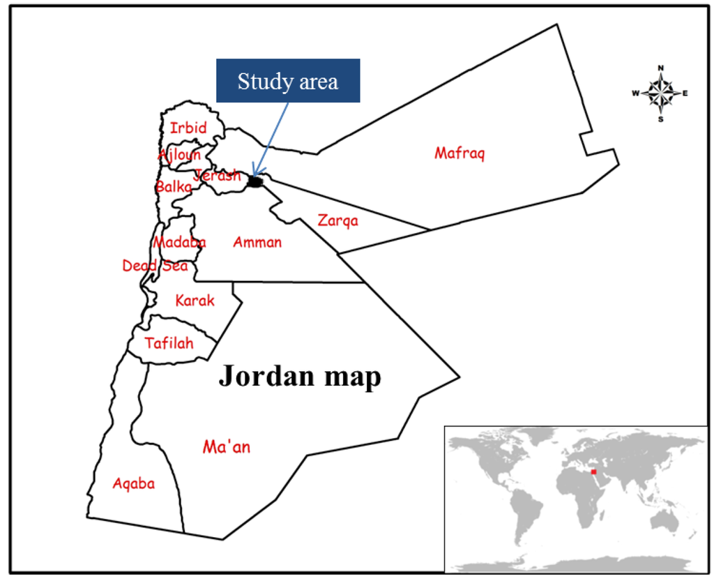
Figure 1. Location map of the study area.

A benchmark site for HSF-CW treatment systems was established in 2008. The system was designed to capture and store the partially-treated municipal wastewater effluent in an influent holding pond, and then re-treat it through HSF-CW beds. The outlet water from HSF-CW beds was stored in another effluent-holding pond and then used for irrigating forest trees. The influent and effluent holding ponds had capacities of 300 m³ and 150 m³, respectively. The HSF-CW system was comprised of 17 sub-surface HSF-CWs. The mean hydraulic residence time was two days. The partially treated municipal wastewater was the only available source of irrigation in this research station and therefore selected as the influent of our HSF-CWs.

2.2. Treatment System Design

The test site for the HSF-CW was divided into two main categories: (1) nine long beds with dimensions of 9.5 m × 1.7 m × 0.8 m (L × W × D). Coarse volcanic tuff (10–20 mm in diameter) was used as the wetland media. Three of the beds were planted with the reed plant Phragmites australis and three of the beds were planted with the kenaf plant Hibiscus cannabinus. The remaining three beds were left without vegetation and were used as controls. (2) Eight short beds with dimensions of 6.5 m × 2.5 m × 0.8 m (L × W × D); four beds were filled with coarse volcanic tuff media (10–20 mm in diameter) and the other four beds were filled with fine volcanic tuff (4–8 mm in diameter). Two of the beds filled with fine media and two of the beds filled with coarse media were planted with reed plants; the remaining four beds did not have vegetation and were used as controls. The area dimension and field facilities were the major variables that controlled the distribution of the treatments discussed above. A schematic of the experimental layout is shown in Figure 2. In the middle of each bed, a tube was installed to facilitate daily measurements of the water temperature. All long and short beds were designed to have the same volume (13 m³ for each bed). The total HSF-CW volume and surface area was 221 m³ and 275 m², respectively. The reeds were planted in November 2008 and removed at the end of the study in November 2011; the planting density was nine rhizomes per square meter. Kenaf is an annual summer crop and was planted in three seasons in 2009, 2010, and 2011 from May until November, with 20 transplants per square meter.

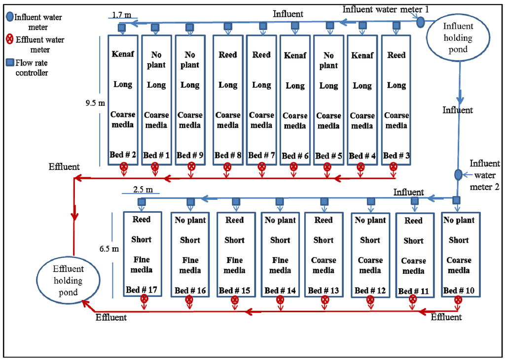
Figure 2. The horizontal sub-surface flow constructed wetland treatment (HSF-CW) system layout.

Figure 2. The horizontal sub-surface flow constructed wetland treatment (HSF-CW) system layout.

In this study, we use the following abbreviations: long (L) bed, short (S) bed, coarse (C) media, and fine (F) media. Reeds, kenaf, and no vegetation will be referred to as R, K, and N, respectively. For example, the long bed with coarse media planted with reeds will be referred to as (LCR) and likewise for all of the treatments discussed above.

2.3. Wastewater Quality Monitoring

The HSF-CW beds’ influent and effluent water were sampled and analyzed by the Jordanian National Center for Agricultural Research and Extension on a bimonthly basis which lasted for 18 months from November 2008 until August 2011. In all, 327 water samples were collected and analyzed for 21 water quality parameters.

The chemical and biological characteristics of wastewater used in this study were: Biological Oxygen Demand (BOD₅), Chemical Oxygen Demand (COD), pH, Electrical Conductivity (EC), Total Suspended Solid (TSS), FC, sulfate (SO4²⁻), magnesium (Mg²⁺), calcium (Ca²⁺), chloride (Cl⁻), sodium (Na⁺), potassium (K⁺), zinc (Zn), cadmium (Cd), cobalt (Co), chromium (Cr), lead (Pb), arsenic (As), phosphorus (P), carbonates (CO³⁻), and bicarbonates (HCO³⁻). The samples were analyzed according to the Standard Methods for the Examination of Water and Wastewater [11]. Details about the sampling procedure, preparations, and instruments are available in the manual [12]. For each water quality parameter, the removal efficiency (%) was calculated based on mass flow difference between the effluent and influent relative to the influent.

2.4. Wastewater Flow Rates and Distribution

Two water meters were used to measure the influent flow rates, each of them located in the main influent supply line as shown in Figure 2. Influent flow rate was controlled to be the same for all the beds through an identical flow rate controller with 17 feed lines, each one installed at the entry point of each bed. Calibration of water flow for even distribution was done before starting up the system. The mean of the two influent water meter readings divided by 17 was used to determine the influent flow rate for each bed. Due to water shortage, our total wastewater share varied from 35 m³·day⁻¹ in the winter seasons to 25 m³·day⁻¹ in the summer seasons, as regulated by the governmental water conservation policy.

An additional water meter and controller for 17 outlet lines were used for effluent flow rate measurement; each one was installed at the end of the bed. However, since the effluent flow rate from each bed was very low the water meters did not work properly. Therefore, we manually measured the effluent flows, and collected two-hour composite effluent samples for each bed. We repeated this measurement six times for each bed, three times in the winter seasons and the other three in the summer seasons.

2.5. Statistical Analyses

We used the Statistical Package for the Social Sciences (SPSS 16) software to conduct statistical analyses. Coinciding with our experimental design and goals, the Kruskal-Wallis test was used to conduct our comparisons. The first comparison was performed between the influent and effluent of each bed. The effluents of LCN, LCK, and LCR were compared as a group 1. Likewise, SCN was compared to SCR as a group 2, SFN to SFR as a group 3, and SC to SF as a group 4. SC and SF media were calculated as SC equals the mean of (SCN and SCR) and SF equals the mean of (SFN and SFR). Moreover, the effluents of LCR were compared to SCR, and the effluents of LCN were compared to SCN to figure out the differences between long and short beds efficiency. Significance was recognized when α <0.05. All “significant differences” mentioned later in this study indicate statistical differences.

2.6. Climate Data

Weather data were collected from the Al-Samra meteorological station, which is the closest weather station to our field test site.

3. Results

Influent water was fed continuously to the beds. The HSF-CW overall mean influent flow was 28 m³·day⁻¹. After it passed through the beds, the effluent was reduced to 23 m³·day⁻¹ with an overall loss of 17%. Mean daily influent and effluent flow rates for each bed are shown in Table 1. In the summer season, the reed, kenaf, and unplanted beds had water losses of 45%, 30%, and 6%, respectively. During the study period, the mean monthly temperature ranged from 9–29 °C. The long-term mean of the monthly temperature ranged from 11.9–24.2 °C (according to the Al-Samra meteorological station data). The range of the monthly water temperature in the beds was 8–24 °C with a mean of 14 °C. The influent pH ranged from 7.2–8.7 with a mean of 7.9. The mean pH of the effluents ranged from 7.5–7.8.

Table 1. Mean daily influent and effluent flow rates for each bed.

Type of Bed	Influent (m3/day)	Effluent (m3/day)	Percentage of Losses (%)
			In the Summer Seasons	In the Winter Seasons	In All the Study Period
Reed bed	1.62	1.15	45	17	29.4
Kenaf bed	1.62	1.37	30	3.2	15.5
Unplanted bed	1.62	1.56	6	2.8	4.0
All the beds	27.62	23.07	26.9	8.6	16.5

Table 1. Mean daily influent and effluent flow rates for each bed.

Type of Bed	Influent (m3/day)	Effluent (m3/day)	Percentage of Losses (%)
			In the Summer Seasons	In the Winter Seasons	In All the Study Period
Reed bed	1.62	1.15	45	17	29.4
Kenaf bed	1.62	1.37	30	3.2	15.5
Unplanted bed	1.62	1.56	6	2.8	4.0
All the beds	27.62	23.07	26.9	8.6	16.5

3.1. HSF-CW Performance

The results of BOD₅, COD, TSS, and P concentration, mass flow, fecal coliform count, and BOD₅/COD are available in

Table A1. The results of BOD₅, COD, TSS, and P concentration, mass flow, fecal coliform count, and BOD₅/COD.

Parameters	Measurements	Influent	Effluent *
			Long Beds			Short Beds				Short Beds
			Coarse Media			Coarse Media		Fine Media		Coarse1 Media	Fine2 Media
			No Plant	Kenaf	Reed	No Plant	Reed	No Plant	Reed
			Group 1			Group 2		Group 3		Group 4
	Mean flow per bed L·day−1	1600	1560	1400	1100	1560	1100	1560	1100	1330	1330
	BOD/COD	0.45	0.38	0.39	0.36	0.46	0.39	0.43	0.41	0.43	0.42
BOD5	Mean concentration mg·L−1	142	72	72	69	91	79	73	68	85	71
	Number of samples	27	41	42	41	22	22	22	22	40	40
	Concentration’s standard deviation	53	43	41	41	38	29	34	31	35	34
	Mean mass flow g·day−1	227	112	101	76 G1	142	87 G2	114	75 G3	114	93 G4
	Mass flow’s standard deviation	85	64	56	40	59	32	54	34	50	48
COD	Mean concentration mg·L−1	316	188	184	191	199	201	171	167	200	169
	Number of samples	27	38	38	38	24	24	24	23	48	47
	Concentration’s standard deviation	119	114	126	94	83	82	78	76	82	80
	Mean mass flow g·day−1	505	294	258	210	311	221	266	184	266	225
	Mass flow’s standard deviation	190	160	177	104	130	91	122	83	109	102
TSS	Mean concentration mg·L−1	72	32	30	28	25	22	26	38	23	32
	Number of samples	37	53	54	53	34	34	34	34	68	68
	Concentration’s standard deviation	59	24	18	22	17	16	18	63	16	47
	Mean mass flow g·day−1	115	50	42	31	38	24	40	42	31	42
	Mass flow’s standard deviation	94	38	25	25	27	17	28	69	22	62
P	Mean concentration mg·L−1	14.3	9.1	8.9	7.4	9.6	8.0	6.2	5.3	8.8	5.7G4
	Number of samples	37	53	54	53	34	34	34	34	68	68
	Concentration’s standard deviation	3.1	4.2	4.1	4.1	3.8	3.4	4.1	3.6	3.6	3.9
	Mean mass flow g·day−1	23	14	12	8 G1	15	9 G2	10	6 G3	12	8 G4
	Mass flow’s standard deviation	5.0	6.5	5.8	4.5	5.9	3.7	6.4	4.0	4.8	5.1
FC	Mean (Log10 CFU/100 mL)	5.2	4.8	4.7	4.7	4.6	4.3	4.0	4.0	4.4	4.1 G4
	Standard deviation (Log10 CFU/100 mL)	1.0	1.1	1.0	1.3	1.0	1.0	1.1	0.9	1.0	1.0
	Number of samples	30	47	48	47	26	26	26	26	52	52
	Standard deviation of FC counts	224,186	147,225	116,745	209,638	51,898	36,322	28,130	47,156	43,859	43,362

* All the effluents were significantly (p < 0.05) lower than the influent, for the same parameter. (G1: significant differences (p < 0.05) compared to others in Group 1, for the same parameter. G2: significant differences (p < 0.05) compared to others in Group 2, for the same parameter. G3: significant differences (p < 0.05) compared to others in Group 3, for the same parameter. G4: significant differences (p < 0.05) compared to others in group 4, for the same parameter. 1: Short coarse media = mean of (short bed, coarse media, no plant-beds) and (short bed, coarse media, reed-beds). 2: Short fine media = mean of (short bed, fine media, no plant-beds) and (short bed, fine media, reed-beds).

. Results of removal efficiencies and fecal coliform reduction are shown in Table 2. The overall removal efficiency of BOD₅ and COD were 55% and 51%, respectively. The different HSF-CW treatments yielded different removal efficiencies. BOD₅ removal efficiency ranged from 37% under SCN conditions to 67% under SFR conditions. In addition, the removal efficiency of COD ranged from 38% for SCN to 64% for SFR. Reed was significantly more efficient than kenaf and unplanted beds in reducing BOD₅, and no significant differences were observed among all three vegetation conditions in reducing COD. There were no significant differences between the long and short beds in removing both parameters. BOD and COD removal rates were not affected by the bed dimensions. A comparison between fine and coarse media indicates that the effluent’s BOD₅ content from the fine media was significantly lower than it was from the coarse media. The fine media was also more efficient than the coarse media in removing COD. However, there were no significant differences between the effluent of the fine and coarse media.

The concentration and mass flow of TSS in the effluent from all of the treatments was significantly lower than that in the influent. The overall removal efficiency of TSS was 67%. TSS removal efficiency ranged from 56% for LCN to 79% in SCR. TSS removal was not affected by the bed dimensions.

The fecal coliform count in the effluent of all HSF-CW treatments was significantly lower than in the influents. The mean log reduction of fecal coliform was 0.8 and ranged from 0.4 for LCN to 1.2 for SFN and SFR. The fecal coliform in the effluent of the fine media was significantly lower than in the coarse media, however there were no significant differences among reed, kenaf, and unplanted beds in removing fecal coliform.

The HSF-CW effluent’s phosphorus concentration and mass flow were significantly reduced compared with that of the influent. The overall phosphorus removal efficiency was 55%. The highest removal efficiency was 75% in SFR; the lowest removal efficiency was 35% in SCN. A comparison between the fine and coarse media indicates that the phosphorus in the effluent from the fine media was significantly lower than from the coarse media. The mass flow of phosphorus in the reed effluent was significantly lower than from the kenaf and unplanted beds. In addition, there were no significant differences between long and short beds in P removal. Phosphorus had a regular behavior during the test period, as revealed by the relatively low standard deviation in Table A1.

Table 2. BOD₅, COD, TSS, Fecal Coliform, and P removal.

Parameter	Long Beds			Short Beds				Short Beds
	Coarse Media			Coarse Media		Fine Media		Coarse 1 Media	Fine 2 Media
	No Plant	Kenaf	Reed	No Plant	Reed	No Plant	Reed
	Group 1			Group 2		Group 3		Group 4
BOD5
Mass flow removal * efficiency (%)	51	56	66G1	37	62G2	50	67G3	50	59G4
Number of samples	41	42	41	22	22	22	22	40	40
COD
Mass flow removal * efficiency (%)	42	49	58	38	56	47	64	47	55
Number of samples	38	38	38	24	24	24	23	48	47
TSS
Mass flow removal* efficiency (%)	56	64	73	67	79	65	64	73	63
Number of samples	53	54	53	34	34	34	34	68	68
P
Mass flow removal * efficiency (%)	38	46	64G1	35	61G2	58	75G3	49	67G4
Number of samples	53	54	53	34	34	34	34	68	68
FC
Log reduction *	0.4	0.5	0.5	0.6	0.9	1.2	1.2	0.8	1.1G4
Number of samples	47	48	47	26	26	26	26	52	52

(1) * All the effluents were significantly (p <0.05) lower than the influent, for the same parameter. (G1: significant differences (p < 0.05) compared to others in group 1, for the same parameter. G2: significant differences (p < 0.05) compared to others in group 2, for the same parameter.G3: significant differences (p < 0.05) compared to others in group 3, for the same parameter. G4: significant differences (p < 0.05) compared to others in group 4, for the same parameter). (2) 1: Short coarse media = mean of (short bed, coarse media, no plant- beds) and (short bed, coarse media, reed-beds). 2: Short fine media = mean of (short bed, fine media, no plant- beds) and (short bed, fine media, reed-beds).

Table 2. BOD₅, COD, TSS, Fecal Coliform, and P removal.

Parameter	Long Beds			Short Beds				Short Beds
	Coarse Media			Coarse Media		Fine Media		Coarse 1 Media	Fine 2 Media
	No Plant	Kenaf	Reed	No Plant	Reed	No Plant	Reed
	Group 1			Group 2		Group 3		Group 4
BOD5
Mass flow removal * efficiency (%)	51	56	66G1	37	62G2	50	67G3	50	59G4
Number of samples	41	42	41	22	22	22	22	40	40
COD
Mass flow removal * efficiency (%)	42	49	58	38	56	47	64	47	55
Number of samples	38	38	38	24	24	24	23	48	47
TSS
Mass flow removal* efficiency (%)	56	64	73	67	79	65	64	73	63
Number of samples	53	54	53	34	34	34	34	68	68
P
Mass flow removal * efficiency (%)	38	46	64G1	35	61G2	58	75G3	49	67G4
Number of samples	53	54	53	34	34	34	34	68	68
FC
Log reduction *	0.4	0.5	0.5	0.6	0.9	1.2	1.2	0.8	1.1G4
Number of samples	47	48	47	26	26	26	26	52	52

(1) * All the effluents were significantly (p <0.05) lower than the influent, for the same parameter. (G1: significant differences (p < 0.05) compared to others in group 1, for the same parameter. G2: significant differences (p < 0.05) compared to others in group 2, for the same parameter.G3: significant differences (p < 0.05) compared to others in group 3, for the same parameter. G4: significant differences (p < 0.05) compared to others in group 4, for the same parameter). (2) 1: Short coarse media = mean of (short bed, coarse media, no plant- beds) and (short bed, coarse media, reed-beds). 2: Short fine media = mean of (short bed, fine media, no plant- beds) and (short bed, fine media, reed-beds).

3.2. Changes in the EC, Major Anions, and Cations

The EC in the effluent from all of the treatments was significantly higher than in the influent. The overall mean EC increase was 16% which matched with the water loss. EC analysis results are given in Figure 3. The EC in the effluents of the long beds planted with reed was significantly higher than those planted with kenaf or unplanted beds. Moreover, there were no significant differences between the EC values for the fine or coarse media.

The results of the calcium, magnesium, sodium, potassium, chloride, sulfate, carbonates, and bicarbonates mass flow changes are shown in Table 3, whereas the results of concentration and mass flow are available in

Table A2. Major anions, cations, micronutrients, and heavy metals in the influent and treated effluents.

Parameters		Influent	Effluent
			Long Beds			Short Beds				Short Beds
			Coarse Media			Coarse Media		Fine Media		Coarse1 Media	Fine2 Media
			No Plant	Kenaf	Reed	No Plant	Reed	No Plant	Reed
			Group 1			Group 2		Group 3		Group 4
	Mean flow per bed L·day−1	1600	1560	1400	1100	1560	1100	1560	1100	1330	1330
	Number of samples	35	50	51	50	32	32	32	32	64	64
Ca2+	Mean concentration mg·L−1	70	90 *	99*	138*G1	91*	111 *,G2	99*	148 *,G3	101*	124 *,G4
	Concentration’s standard deviation	17	31	42	75	31	44	44	86	39	72
	Mean mass flow g·day−1	112	140 *	138 *	151*	142*	122 *	155 *	163 *	134 *	164 *,G4
	Mass flow’s standard deviation	27	49	58	83	49	48	68	95	52	96
Mg2+	Mean concentration mg·L−1	52	53	55	68 *,G1	57	57	59	72*	57	65*G4
	Concentration’s standard deviation	10	14	17	28	14	15	23	37	14	31
	Mean mass flow g·day−1	83	83	77	75	88	63 *,G2	92	79	76	87G4
	Mass flow’s standard deviation	15	22	24	31	21	16	36	40	19	41
Na+	Mean concentration mg·L−1	303	330	344 *	422 *,G1	339 *	380 *,G2	342 *	429 *,G3	359*	386 *
	Concentration’s standard deviation	53	85	103	153	87	98	97	157	94	137
	Mean mass flow g·day−1	485	515	482	465	529 *,G2	417 *	534	472	478	513
	Mass flow’s standard deviation	86	132	145	168	136	107	151	173	125	182
K+	Mean concentration mg·L−1	39	47 *	47 *	47 *	46 *	47 *	50*	50*	46 *	50 *
	Concentration’s standard deviation	6	8	9	13	8	10	15	17	9	16
	Mean mass flow g·day−1	62	73 *,G1	65	51 *,G1	71 *,G2	52*	78 *,G3	55	62	67
	Mass flow’s standard deviation	9	12	12	14	12	11	23	18	12	21
Cl−	Mean concentration mg·L−1	408	443	465 *	588 *,G1	461 *	521 *,G2	477 *	619 *,G2	491*	548 *,G2
	Concentration’s standard deviation	57	98	123	247	99	151	155	278	131	235
	Mean mass flow g·day−1	653	691	651	648	718 *,G2	573 *	744 *	681	653	729
	Mass flow’s standard deviation	92	153	172	271	154	167	242	306	174	312
SO42−	Mean concentration mg·L−1	137	206	220 *	349 *,G1	212 *	270 *,G2	249*	369 *,G3	241 *	309 *
	Concentration’s standard deviation	108	192	196	257	162	178	184	263	172	233
	Mean mass flow g·day−1	220	322	307	384*	331*	297	389*	406 *	320*	411 *
	Mass flow’s standard deviation	173	299	275	283	253	196	287	290	228	310
HCO3	Mean concentration mg·L−1	422	414 G1	436	476	413	447 G2	389	471 G3	430	430
	Concentration’s standard deviation	96	89	94	160	76	106	97	157	93	136
	Mean mass flow g·day−1	676	645 G1	610*	524 *,G1	644	492 *,G2	607	518 *,G3	572*	572 *
	Mass flow’s standard deviation	154	140	131	176	119	117	151	173	124	181
CO3−	Mean concentration mg·L−1	21	22	21	17	22	18	23	21	20	22
	Concentration’s standard deviation	15	15	16	16	16	17	17	15	17	16
	Mean mass flow g·day−1	34	38	35	26 G1	39	27 G2	42	27 G3	33	34
	Mass flow’s standard deviation	24	21	20	16	24	17	23	13	20	18
Cd	Mean concentration mg·L−1	0.012	0.010	0.010	0.009	0.010	0.010	0.012	0.011	0.010	0.011
	Concentration’s standard deviation	0.01	0.01	0.01	0.01	0.01	0.01	0.01	0.01	0.01	0.01
	Mean mass flow g·day−1	0.019	0.016	0.013*	0.010 *,G1	0.015	0.011 *	0.018	0.012 *	0.013 *	0.015 a
	Mass flow’s standard deviation	0.02	0.01	0.01	0.01	0.01	0.01	0.02	0.01	0.01	0.01
Co	Mean concentration mg·L−1	0.027	0.022	0.018	0.018	0.022	0.025	0.024	0.028	0.023	0.026
	Concentration’s standard deviation	0.04	0.03	0.03	0.02	0.03	0.03	0.03	0.04	0.03	0.03
	Mean mass flow g·day−1	0.043	0.035	0.025	0.020 *,G1	0.034	0.027	0.037	0.031	0.031	0.035
	Mass flow’s standard deviation	0.06	0.05	0.04	0.03	0.04	0.03	0.05	0.04	0.04	0.05
Zn	Mean concentration mg·L−1	0.06	0.04 *	0.03 *	0.05 G1	0.05	0.04	0.03 *	0.03 *	0.04	0.03 *G4
	Concentration’s standard deviation	0.04	0.05	0.02	0.05	0.05	0.05	0.04	0.04	0.05	0.04
	Mean mass flow g·day−1	0.1	0.06 *	0.04 *	0.05 *	0.07	0.04 *	0.04*	0.03 *	0.06 *	0.04 *
	Mass flow’s standard deviation	0.07	0.07	0.03	0.05	0.08	0.05	0.07	0.05	0.06	0.06

* The effluents were significantly (p <0.05) different than the influent. (G1: significant differences (p < 0.05) compared to others in Group 1, for the same parameter. G2: significant differences (p < 0.05) compared to others in Group 2, for the same parameter. G3: significant differences (p < 0.05) compared to others in Group 3, for the same parameter. G4: significant differences (p < 0.05) compared to others in Group 4, for the same parameter. 1: Short coarse media = mean of (short bed, coarse media, no plant-beds) and (short bed, coarse media, reed-beds). 2: Short fine media = mean of (short bed, fine media, no plant-beds) and (short bed, fine media, reed-beds).

. The most pronounced changes were the levels of calcium and sulfate.

Calcium mass flow and concentration in the effluent from all of the treatments was significantly higher than in the influent. The overall mean increase in calcium mass flow was 30%. The calcium concentration in the effluent of the beds planted with reed was significantly higher than that in beds planted with kenaf or unplanted. Moreover, calcium mass flow and concentration in the effluent of SF was significantly higher than in SC.

The sulfate concentration and mass flow in the effluent from all of the treatments were significantly higher than those in the influent, except for LCN, LCK, and SCR showing no significant increases in their effluent’s sulfate mass flow. The concentration of sulfate in the effluent of the long and short beds planted with reed was significantly higher than in beds planted with kenaf or unplanted beds. Moreover, there were no significant differences between the effluent’s sulfate levels in the fine and coarse media or even among reed, kenaf, and unplanted effluents.

Relatively, all other elements analyzed showed some changes after treatment, but the differences were not pronounced or significant as compared to calcium and sulfate. The water loss, plant uptakes and releases, have all contributed to many of the changes, along with other unknown factors.

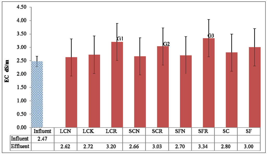
Figure 3. The mean electrical conductivity (EC) in influent and effluent of various treatments. (1) EC in all the effluents were significantly (p < 0.05) higher than the influent. (2) G1: significant differences (p < 0.05) among (LCN, LCK and LCR) effluents; G2: significant differences (p < 0.05) between (SCR and SCN) effluents; G3: significant differences (p < 0.05) between (SFN and SFR) effluents. (3) Abbreviation in the X-axis are available in “Treatment System Design” section.

Figure 3. The mean electrical conductivity (EC) in influent and effluent of various treatments. (1) EC in all the effluents were significantly (p < 0.05) higher than the influent. (2) G1: significant differences (p < 0.05) among (LCN, LCK and LCR) effluents; G2: significant differences (p < 0.05) between (SCR and SCN) effluents; G3: significant differences (p < 0.05) between (SFN and SFR) effluents. (3) Abbreviation in the X-axis are available in “Treatment System Design” section.

Table 3. Mass flow changes (%) for major anions, cations, micronutrients, and heavy metals.

Parameters	Long Beds			Short Beds				Short Beds
	Coarse Media			Coarse Media		Fine Media		Coarse1 Media	Fine2 Media
	No Plant	Kenaf	Reed	No Plant	Reed	No Plant	Reed
	Group 1			Group 2		Group 3		Group 4
Ca2+	+25 *	+23 *	+35 *	+27 *	+9 *	+38 *	+45 *	+20*	+47 *,G4
Mg2+	0	−7	−10	+6	−24 *,G2	+11	−5	− 9	+4 G4
Na+	+6	−1	−4	+9*G2	−14*	+10	−3	−2	+6
K+	+17 *,G1	+5	−18 *,G1	+15 *,G2	−17*	+26 *,G3	−11	0	+8
Cl−	+6	0	−1	+10 *,G2	−12*	+14*	+4	0	+12
SO42−	+46	+40	+74 *	+50 *	+35	+77*	+85 *	+46 *	+87 *
HCO3−	−5 G1	−10 *	−23 *,G1	−5	−27 *,G2	−10	−23 *,G3	−15*	−15 *
CO3−	+11	+3	−23 G1	+16	−20 G2	+22	−19G3	−2	0
Cd	−19	−33 *	−48 *,G1	−24	−45 *	−9	−38 *	−35 *	−24 a
Co	−19	−42	−54 *,G1	−21	−37	−13	−28	−28	−19
Zn	−40 *	−59 *	−50 *	−30	−57 *	−59*	−69 *	−44 *	−64 *

Notes: (1) Mass flow changes: (+) increases in the mass flow. (−) decreases in the mass flow. (2) * The effluents were significantly (p < 0.05) different than the influent. (G1: significant differences (p < 0.05) compared to others in Group 1, for the same parameter. G2: significant differences (p < 0.05) compared to others in Group 2, for the same parameter. G3: significant differences (p < 0.05) compared to others in Group 3, for the same parameter. G4: significant differences (p < 0.05) compared to others in Group 4, for the same parameter). (3) 1: Short coarse media = mean of (short bed, coarse media, no plant-beds) and (short bed, coarse media, reed-beds). 2: Short fine media = mean of (short bed, fine media, no plant-beds) and (short bed, fine media, reed-beds).

Table 3. Mass flow changes (%) for major anions, cations, micronutrients, and heavy metals.

Parameters	Long Beds			Short Beds				Short Beds
	Coarse Media			Coarse Media		Fine Media		Coarse1 Media	Fine2 Media
	No Plant	Kenaf	Reed	No Plant	Reed	No Plant	Reed
	Group 1			Group 2		Group 3		Group 4
Ca2+	+25 *	+23 *	+35 *	+27 *	+9 *	+38 *	+45 *	+20*	+47 *,G4
Mg2+	0	−7	−10	+6	−24 *,G2	+11	−5	− 9	+4 G4
Na+	+6	−1	−4	+9*G2	−14*	+10	−3	−2	+6
K+	+17 *,G1	+5	−18 *,G1	+15 *,G2	−17*	+26 *,G3	−11	0	+8
Cl−	+6	0	−1	+10 *,G2	−12*	+14*	+4	0	+12
SO42−	+46	+40	+74 *	+50 *	+35	+77*	+85 *	+46 *	+87 *
HCO3−	−5 G1	−10 *	−23 *,G1	−5	−27 *,G2	−10	−23 *,G3	−15*	−15 *
CO3−	+11	+3	−23 G1	+16	−20 G2	+22	−19G3	−2	0
Cd	−19	−33 *	−48 *,G1	−24	−45 *	−9	−38 *	−35 *	−24 a
Co	−19	−42	−54 *,G1	−21	−37	−13	−28	−28	−19
Zn	−40 *	−59 *	−50 *	−30	−57 *	−59*	−69 *	−44 *	−64 *

Notes: (1) Mass flow changes: (+) increases in the mass flow. (−) decreases in the mass flow. (2) * The effluents were significantly (p < 0.05) different than the influent. (G1: significant differences (p < 0.05) compared to others in Group 1, for the same parameter. G2: significant differences (p < 0.05) compared to others in Group 2, for the same parameter. G3: significant differences (p < 0.05) compared to others in Group 3, for the same parameter. G4: significant differences (p < 0.05) compared to others in Group 4, for the same parameter). (3) 1: Short coarse media = mean of (short bed, coarse media, no plant-beds) and (short bed, coarse media, reed-beds). 2: Short fine media = mean of (short bed, fine media, no plant-beds) and (short bed, fine media, reed-beds).

3.3. Changes in Micronutrients and Heavy Metals

The removal efficiency of cadmium, cobalt, and zinc in the influent and effluent are shown in Table 3, whereas results of the concentration and mass flow are available in Table A2. There were no significant differences between the cadmium concentration in the effluent and influent of each bed. Cadmium mass flow in the effluent from the reed and kenaf was significantly lower than in the influent. The overall mass flow removal efficiency of cadmium was 31% and ranged from 9% in the SFN to 48% in the LCR. Cobalt mass flow in the effluent from LCR was significantly lower than in the influent, cobalt removal efficiency in that bed reached 54%. The overall removal efficiency of cobalt was 29% and ranged from 13% in SFN to 54% in LCR. Zinc mass flow in the effluent from all of the HSF-CWs was significantly lower than in the influent, except the case of SCN that had insignificant reduction. The overall removal efficiency of zinc was 52% and ranged from 30% in SCN to 69% in SFR. There was no significant difference among all other parameters (i.e., bed type, media type, and vegetation type [including unplanted beds]) in terms of removing zinc.

There was also no significant difference between the influent and effluent chromium, lead, or arsenic in either concentration or mass flow levels.

4. Discussion

This study has provided long-term field test data with statistical analysis on various HSF-CW in an arid environment. The data show that all HSF-CW beds were moderately efficient in removing BOD₅, COD, TSS, and phosphorus. The mass flow reduction, instead of concentration changes, clearly shows the actual performance of all beds. The highest BOD₅ and COD removal percentages were achieved in the case of reed with fine media. This result corresponds well with the results of Reed [13] and Rani [14], who found that fine media provides more surface area for treatment and better development of plant roots. Previous studies revealed that the BOD₅ and COD removal are through aerobic and anoxic degradation of organic compounds by microorganisms on plant roots and the media surface [5,14]. Sedimentation and filtration also may contribute to BOD₅ removal [15]. Our BOD₅ and COD removal efficiencies were generally lower than those found in earlier studies; for example, Göçmez [4] found BOD₅ and COD removal efficiencies of 71% and 63%, respectively. A worldwide survey conducted by Puigagut [16] found that the BOD₅ removal efficiencies varied between 75% and 93%. This may be due to the lower levels of degradable organic matter in our influent (low BOD₅/COD ratios are shown in Appendix Supplementary Table S1), as well as the anoxic condition inside the beds. Most of the easily degradable organic matters were removed before entering HSF-CW since our influent was partially biodegraded municipal wastewater.

The removal of suspended solids is accomplished via sedimentation and filtration in addition to biodegradation, therefore the void space might have some influence [2,17]. TSS removal was not affected by the HSF-CW bed dimensions, this result agrees well with the results of Reed [13]. In previous studies, Rani [14] compared horizontal- and vertical-subsurface wetlands and found that TSS removal was slightly higher in the horizontal case but the removal efficiency exceeded 96% in both systems. In contrast, the removal performances off TSS ranged from 56.62% and 91.04% in Göçmez’s four year study [4]. However, the different media types and sizes must have impacted TSS results in various studies.

In our study, the fecal coliform in the effluent of the fine media was significantly lower than in the coarse media, and there were no significant differences among the reed, kenaf, and unplanted beds in removing fecal coliform. Although other studies have shown higher FC reduction, the differences could be due to test variations [18,19,20].

The removal of phosphorus in wetlands is achieved by plant uptake, adsorption, bacterial removal, and precipitation [14,21]. The highest phosphorus removal efficiency in our HSF-CWs was in the case of reed with fine media. We expected decreases in phosphorus, both in concentration and in mass flow because reed uptakes it as a nutrient. In addition, the large surface area and high contact between the solid phase and the water column in the fine media enhanced phosphorus removal. Phosphorus might precipitate in the form of calcium phosphate, and this could be caused by calcium from dissolved media in our study. Some other studies have shown the importance of contact and contact time between the water phase and solid media [2,13,14,21,22].

Previous studies had higher removal rates of heavy metals than our study [23]. The change of concentration of heavy metals may be due to, in our case, the media adsorption or release, precipitation, pH decreases, and evapoconcentration. Furthermore, plant uptake plays a major role in planted beds since there were significant differences between the planted and unplanted beds in removing cadmium and cobalt. The volcanic tuff media was efficient at removing the zinc from the effluent. This result was also previously shown [24].

Evaporative concentration was a major concern in our study, as it has led to an increase of soluble mineral and EC in the effluents. The EC in the reed bed’s effluent was approximately 20% higher than the other bed’s effluent, which is reasonable since the mean water losses in the reed beds was 29%. In a previous study, EC has changed from −0.60% to −13% after passing through CW with various hydraulic retention times [25], which was attributed to evapotranspiration and/or plant uptake. This attribution could explain our results as well.

Both calcium and sulfate ions increased more significantly than all other ions. In this study, the main source of water-soluble metals is the media material. Our volcanic tuff media, also known as zeolitic tuff and phillipsite is the primary mineral in the tuff [26]. The phillipsite crystal has variable amounts of silicon, aluminum, sodium, potassium, and high calcium oxide level up to 11.51% [26]. Plant uptake led to significant decreases in the potassium mass flow in the effluent of the long and short beds planted with reed, as compared with the beds planted with kenaf or the unplanted beds. Potassium increases in the unplanted beds might have come from the media itself [26]. The higher sulfate level in the HSF-CW’s effluent was probably caused by the dissolution of gypsum [27] and we expected that the gypsum was mixed with our media from its source. To overcome this problem, we suggest to choose a more suitable media, and to avoid using reed plants in HSF-CW beds if used in arid areas, for reed beds show a mean water loss of almost 29%, a figure that reaches 45% in the summer season. We also suggest not to use kenaf plants in HSF-CWs as it is an annual crop with about 16% water loss and its water effluent quality is not any better than that of unplanted beds. The unplanted beds with either fine or coarse media have performed better than the other combinations. Since that combination was vegetation free, it can be categorized as a granular filtration system.

Regarding bed dimensions, our study showed that the bed length did not significantly affect the general performance given the same bed volume and the dimensional ratios we used.

5. Conclusions

• Our horizontal sub-surface flow constructed wetland treatment system has adequately removed BOD₅, COD, TSS, and P. The effluents of the long and short beds of equal bed volume did not show statistically significant differences.
• Reed plants were efficient in removing organic contaminants but they consumed a lot of water and therefore concentrated the effluents. Beds with kenaf plants and beds without plants showed similar quality in their effluents.
• Evaporation caused water losses and concentrated effluents. Therefore the removal efficiencies were compared based on mass flows instead of concentrations.
• Both fine and coarse media without vegetation removed significant amounts of organic contaminants while minimizing water losses to only 4%.
• The unplanted beds with either fine or coarse media acted as granular filters and performed better than other design combinations studied.
• A granular filtration system with media suitable for microbial growth and surface contact with the wastewater is suggested for future implementation. However, further research on constructed wetland in arid areas are still needed concerning evaporation loss, media selection, hydraulic retention time, and related design combinations.

References

- Vymazal, J. Constructed wetlands for wastewater treatment: Five decades of experience. Environ. Sci. Technol. 2010, 45, 61–69. [Google Scholar] [CrossRef] [PubMed]
- Vymazal, J. Natural and Constructed Wetlands: Nutrients, Metals and Management; Backhuys: Trebon, Czech, 2005; Volume 10. [Google Scholar]
- Kivaisi, A.K. The potential for constructed wetlands for wastewater treatment and reuse in developing countries: A review. Ecol. Eng. 2001, 16, 545–560. [Google Scholar] [CrossRef]
- Göçmez, S.; Kayam, Y.; Bilir, Z.L. Constructed Wetlands for Municipal Waste Water Treatment; Case Study of Çakirbeyli Village. In Proceedings of International Sustainable Water and Wastewater Management Symposium, Konya, Turkey, 26–28 October 2010.
- Vymazal, J.; Kröpfelová, L. Wastewater Treatment in Constructed Wetlands with Horizontal Sub-Surface Flow; Springer Science & Business Media: Dordrecht, The Netherlands, 2008; Volume 14. [Google Scholar]
- Diemont, S.A. Mosquito larvae density and pollutant removal in tropical wetland treatment systems in Honduras. Environ. Int. 2006, 32, 332–341. [Google Scholar] [CrossRef] [PubMed]
- Zhang, D.Q.; Jinadasa, K.B.S.N.; Gersberg, R.M.; Liu, Y.; Ng, W.J.; Tan, S.K. Application of constructed wetlands for wastewater treatment in developing countries—A review of recent developments (2000–2013). J. Environ. Manag. 2014, 141, 116–131. [Google Scholar] [CrossRef] [PubMed]
- Vera, I.; Verdejo, N.; Chávez, W.; Jorquera, C.; Olave, J. Influence of hydraulic retention time and plant species on performance of mesocosm subsurface constructed wetlands during municipal wastewater treatment in super-arid areas. J. Environ. Sci. Health Part A 2016, 51, 105–113. [Google Scholar] [CrossRef] [PubMed]
- Department of Statistics (DOS). Jordan in Figures 2010; Issue 13; Department of Statistics: Amman, Jordan, 2011. [Google Scholar]
- Al-Omari, A.; Fayyad, M. Treatment of domestic wastewater by subsurface flow constructed wetlands in Jordan. Desalination 2003, 155, 27–39. [Google Scholar] [CrossRef]
- Standard Methods for the Examination of Water and Wastewater; American Public Health Association, Water Environment Federation: Washington, DC, USA, 1995; p. 19.
- Ryan, J.; Estefan, G.; Rashid, A. Soil and Plant Analysis Laboratory Manual; International center for Agricultural Research in the Dry Areas (ICARDA): Aleppo, Syria, 2001. [Google Scholar]
- Reed, S.C. Subsurface Flow Constructed Wetlands for Wastewater Treatment: A Technology Assessment; EPA 832-R-93-008; United States Environmental Protection Agency, Office of Water (4204): Washington, DC, USA, 1993.
- Rani, S.H.C.; Din, M.F.M.; Yusof, M.B.M.; Shreeshivadasan, C. Overview of Subsurface Constructed Wetlands Application in Tropical Climates. Univers. J. Environ. Res. Technol. 2011, 1, 103–114. [Google Scholar]
- Kiracofe, B.D. Performance Evaluation of the Town of Monterery Wastewater Treatment Plant Utilizing Subsurface Flow Constructed Wetlands. Master’s Thesis, Virginia Polytechnic Institute of State University, Blacksburg, VA, USA, 2000. [Google Scholar]
- Puigagut, J.; Villaseñor, J.; Salas, J.J.; Bécares, E.; García, J. Subsurface-flow constructed wetlands in Spain for the sanitation of small communities: A comparative study. Ecol. Eng. 2007, 30, 312–319. [Google Scholar] [CrossRef]
- Cooper, P.F. Reed Beds and Constructed Wetlands for Wastewater Treatment; WRc Publications: Swindon, UK, 1996. [Google Scholar]
- Decamp, O.; Warren, A. Investigation of Escherichia coli removal in various designs of subsurface flow wetlands used for wastewater treatment. Ecol. Eng. 2000, 14, 293–299. [Google Scholar] [CrossRef]
- Karathanasis, A.; Potter, C.; Coyne, M.S. Vegetation effects on fecal bacteria, BOD, and suspended solid removal in constructed wetlands treating domestic wastewater. Ecol. Eng. 2003, 20, 157–169. [Google Scholar] [CrossRef]
- Mairi, J.P.; Lyimo, T.J.; Njau, K.N. Performance of Subsurface Flow Constructed Wetland for Domestic Wastewater Treatment. Tanzan. J. Sci. 2013, 38, 53–64. [Google Scholar]
- Ohio-EPA. Guidance Document for Small Subsurface Flow Constructed Wetlands with Soil Dispersal System; OAC 3745-42; Ohio Environmental Protection Agency, Division of Surface Water: Columbus, OH, USA, 2007. [Google Scholar]
- Kadlec, R.; Knight, R. Treatment Wetlands; CRC: Baca Raton, FL, USA, 1996. [Google Scholar]
- Sarafraz, S.; Mohammad, T.A.; Noor, M.J.M.M.; Liaghat, A. Wastewater treatment using horizontal subsurface flow constructed wetland. Am. J. Environ. Sci. 2009, 5, 772–778. [Google Scholar]
- Al-Dwairi, R.; Ibrahim, K.; Khoury, H. Occurrences and Properties of Jordanian Zeolites and Zeolitic Tuff; VDM: Saarbrücken, Germany, 2010. [Google Scholar]
- Shuib, N.; Baskaran, K.; Jegatheesan, V. Evaluating the performance of horizontal subsurface flow constructed wetlands using natural zeolite (escott). Int. J. Environ. Sci. Dev. 2011, 2, 311–315. [Google Scholar]
- Al Dwairi, R.A.; Ibrahim, K.M.; Khoury, H.N. Potential use of faujasite–phillipsite and phillipsite–chabazite tuff in purification of treated effluent from domestic wastewater treatment plants. Environ. Earth Sci. 2014, 71, 5071–5078. [Google Scholar] [CrossRef]
- Kuechler, R.; Noack, K.; Zorn, T. Investigation of gypsum dissolution under saturated and unsaturated water conditions. Ecol. Model. 2004, 176, 1–14. [Google Scholar] [CrossRef]
© 2016 by the authors; licensee MDPI, Basel, Switzerland. This article is an open access article distributed under the terms and conditions of the Creative Commons by Attribution (CC-BY) license (http://creativecommons.org/licenses/by/4.0/).