Estimating Sediment Discharge Using Sediment Rating Curves and Artificial Neural Networks in the Shiwen River, Taiwan

Abstract

Sediment in river is usually transported during extreme events related to intense rainfall and high river flows. The conventional means of collecting data in such events are risky and costly compared to water discharge measurements. Hence, the lack of sediment data has prompted the use of sediment rating curves (SRC). The aim of this study is to explore the abilities of artificial neural networks (ANNs) in advancing the precision of stream flow-suspended discharge relationships during storm events in the Shiwen River, located in southern Taiwan. The ANNs used were multilayer perceptrons (MLP), the coactive neurofuzzy inference system model (CANFISM), time lagged recurrent networks (TLRN), fully recurrent neural networks (FRNN) and the radial basis function (RBF). A comparison is made between SRC and the ANNs. Hourly based water and sediment discharge during 8 storms were manually collected and used as inputs for the SRC and the ANNs. Results have shown that the ANN models were superior in reproducing hourly sediment discharge compared to SRC. The findings further suggest that MLP can provide the most accurate estimates of sediment discharge, (R² of 0.903) compared to CANFISM, TLRN, FRNN and RBF. SRC had the lowest R² (0.765), and resulted in underestimations of peak sediment discharge (−47%).

1. Introduction

Taiwan is located in a sub-tropic area and is often subjected to several storms and typhoons during a monsoon season (June to August). The average annual rainfall ranges from 2500 mm/year up to 3000–5000 mm/year in hilly regions. These typhoons induce severe hazards in the form of flooding [1,2]. In comparison to global rivers, the ones in Taiwan have the largest discharge per unit of drainage area, steepest slopes and a minute concentration time [3]. Furthermore, the poor geologic formations (fragile sandstones) of the watersheds, especially in the upstream sections, result in heavy deposition in the downstream regions due to the extreme rainfall events. Subsequently, Taiwanese rivers are among the highest in the world in sediment concentrations [4].

Engineering designs, river basin management, water resources planning, reservoir management and operation all depend on precise calculations/predictions of sediment loads for their successful implementation. Direct sampling of sediment in rivers or reservoirs and sediment transport formulas are among the popular means of estimating sediment loads and their respective transport. While direct measurement is the most preferred and trusted method, it is not always practical during periods of extreme events mainly because of safety reasons and accomplishing such a task is difficult. Besides the above challenge, sediment monitoring programs are expensive and are therefore not frequently performed. Instead, monitoring programs are conducted on selected streams based on their importance. Generally, in most streams, water level is measured, and is converted to water discharge using rating curves. The lack of sediment measurements has prompted the wide adoption of sediment rating curves in predicting sediment load in rivers. A power function relating sediment discharge and water discharge over extended periods (usually more than 10 years) often defines good sediment rating curves. In many instances though, establishing a single association between sediment discharge (Qs) and water discharge (Q) is nearly an impossible task due to the dissimilarities in high flow events discharge and their subsequent sediment concentration levels plus hysteresis [5]. Overall, the appropriateness of regression means to developing good sediment rating curves is influenced by the size and characteristics of sediments in a particular river [6]. There is, however, a concern in applying such approaches in small-scale rivers mainly because the above methods were developed from large rivers. Water energy discharge is generally a good means for estimating sediment transport in huge rivers since these rivers have ample suspended materials for transport. On the contrary, small-scale rivers rely on sporadic precipitation events and their impacts on upland regions.

Periodic and systematic observations of discharge are necessary to comprehend the temporal and spatial variability of rivers. Traditional discharge mensuration methods initially measure cross section areas and velocity. Current meters (like the Price meter) are placed at selected locations in the river to measure velocity. Nevertheless, during flood periods, it is nearly impossible to submerge the meter, even if additional weights are utilized. In addition, the riverbed is highly unstable under high flow conditions due to accelerated erosion and deposition making sound water depth impossible; hence, complicating cross section area measurements. Not only is the riverbed unstable during floods, but flow is highly unsteady too, and there is a great variation between water stage and subsequent discharge. As a result, precise discharge mensuration should be conducted promptly. Besides, the environmental conditions when conducting discharge measurements during flood periods are nowhere near an ideal state. Flood threatens the safety of individuals completing the tasks and often results in a loss of measurement instruments. Therefore, employing current meters under such conditions is less recommended.

The sediment transport process resembles a very complex and non-linear system. Yet, empirical methods (regressions) are continuously used in spite of their shortcomings in depicting the non-linear environment. It is indispensable that non-linear system methods like artificial neural networks (ANNs), which are appropriate for complex and non-linear systems, are adopted. ANNs are proficient in modelling any arbitrary complex non-linear process that relates meteorological data to sediment transport and loads [7]. They have gained popularity over the years in terms of hydrological applications. Beginning in the early 90’s, ANNs have been successful in hydrology fields. They have been applied in rainfall-runoff modeling [8]. Tfwala et al. [9] used a multilayer perceptron and coactive neurofuzzy inference system model to estimate missing stream flow records. Melesse et al. [10] used MLP to predict the suspended load of river systems. Further, several authors have successfully used different types of ANNs, e.g., generalized regression neural network [11], feed forward propagation [12] and time lagged recurrent network [7]. Therefore, the objective of this study is to explore the accuracy of different artificial neural networks (five) in predicting sediment discharge using hourly data collected from 8 typhoon events in Taiwan. These different neural network algorithms are then compared with SRCs, which are currently used in the study area.

2. Materials and Methods

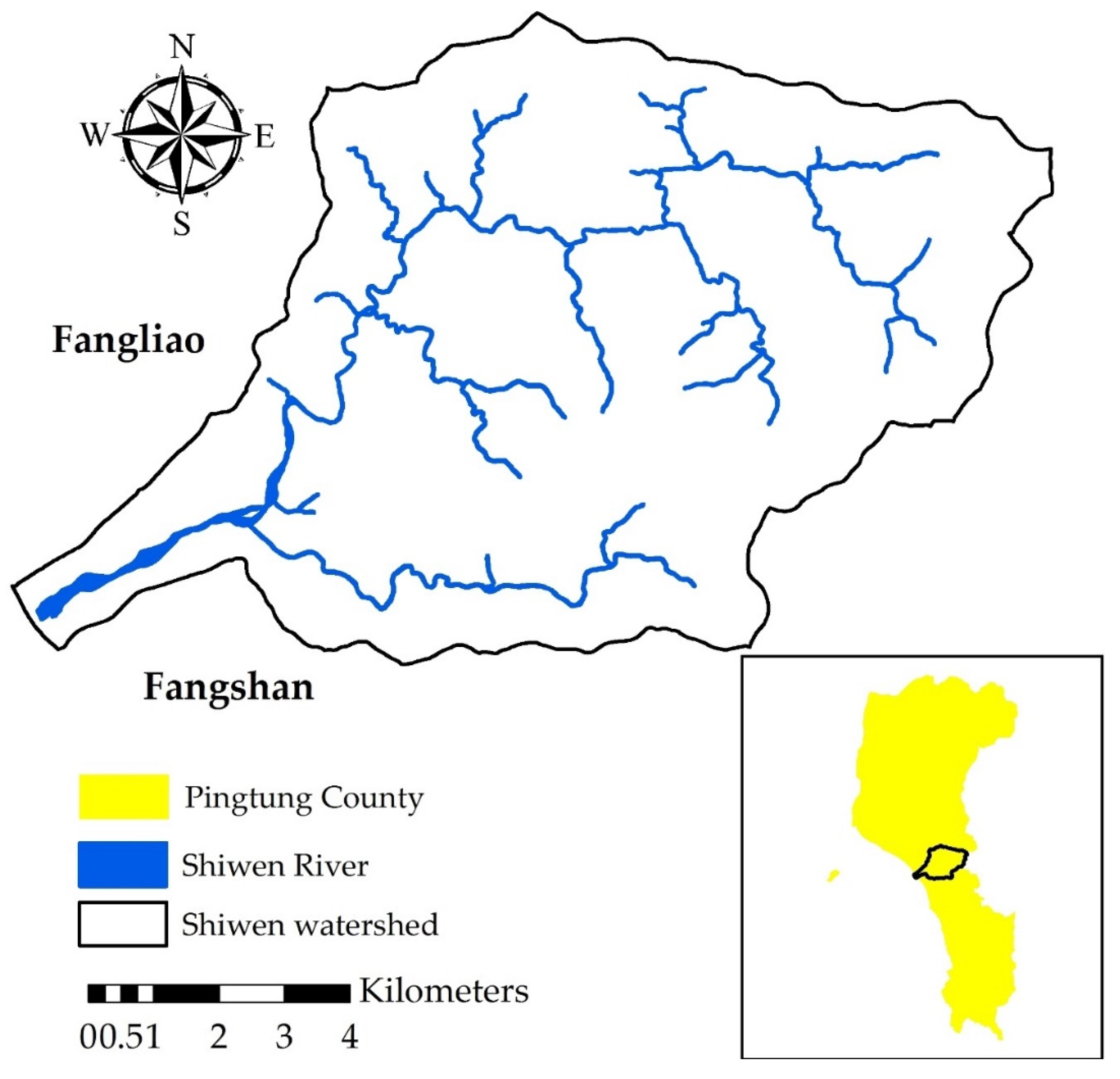
2.1. Study Area

Our study area was in the Shiwen River, located (21°34′48′′ North latitude and 120°47′56′′ East longitude) in the southern part of Taiwan (Figure 1), an area receiving an average of 2300 mm/year. The main stream length is about 22.3 km in a watershed covering about 90 km². The average slope is about 0.03 with a design flood at 1300 m³/s (50-year return period). The watershed is dominated by forests and agricultural activities as shown in Figure 2. Forests occupy about 88% of the watershed, and agriculture about 7%. Built up land within the watershed comprises about 0.1%. The poor geologic characteristics of Taiwanese watersheds [4] combined with the location of agricultural activities in this watershed (Shiwen) have resulted in increased rates of sediment discharge as demonstrated by [2]. Figure 2 shows the location of agricultural fields in close proximity to the main river channel, which could be another source of the accelerated sediment volumes in this river.

Figure 1. Shiwen River watershed.

Figure 1. Shiwen River watershed.

Figure 2. Land use map for the Shiwen watershed.

Figure 2. Land use map for the Shiwen watershed.

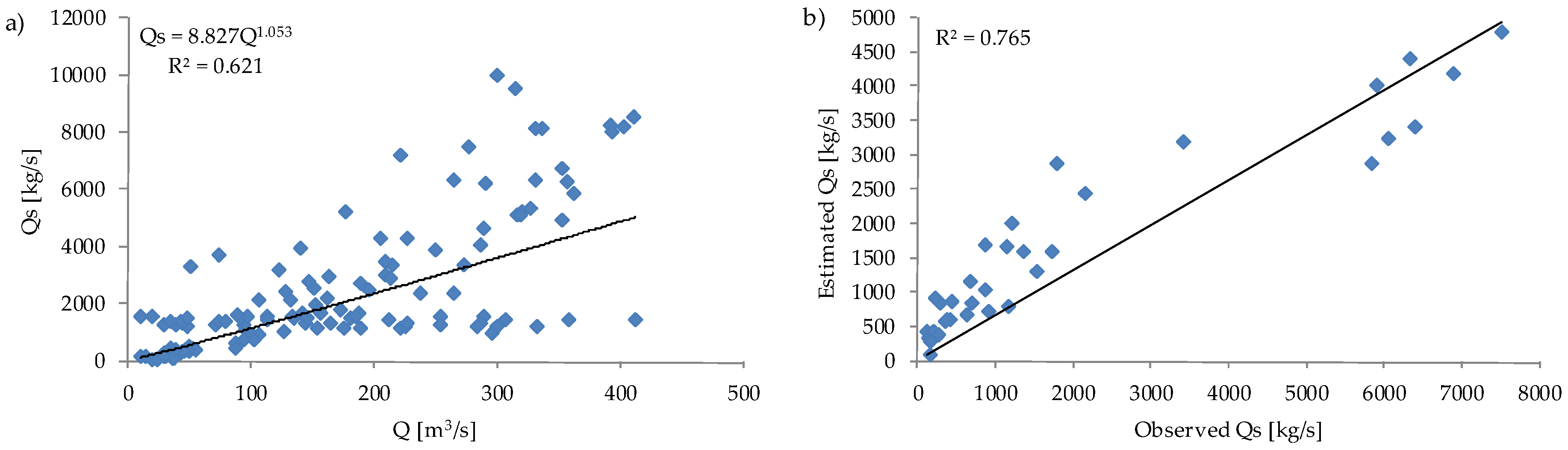
2.2. Sediment Rating Curve

Fluvial data were manually collected on an hourly basis during 8 typhoon events, which occurred between 2012 and 2014. In total, 170 observations were made. These included water velocity, cross section area (for computing discharge) and suspended sediment concentration (SSC). SSC samples were analyzed in the hydraulic laboratory at the National Pingtung University of Science and Technology. Filtration methods, evaporation and weighing of remaining sediments were employed. Analysis results have shown that suspended sediments from the different storms constituted fine sediments (clay to fine sand material) in the range 0.001 to 0.1 mm. To enable comparison between the developed sediment rating curves (SRC) and ANN, the data sets were split into two for training and testing purposes. Therefore, in a data set comprising 170 observations of hourly water discharge and suspended discharge, regression analyses were performed using 80% (136 data sets) for the establishment of a sediment rating curve, employing the most frequently used power function. The remaining 20% (34 data sets) were used for testing the developed SRC in estimating sediment discharge.

2.3. Artificial Neural Networks

ANNs are computational models that mimic how the human brain works [13]. They are made of neurons as basic elements. The neuron will receive a signal (which represents inputs), process it using different ANN configurations, and finally convert tit into results for intepretation. Inputs can be raw data, or outputs from other processing elements (neurons) [14]. For ANNs to be successfully applied, they need to undergo a learning procedure. This procedure can be grouped into either unsupervised or supervised learning. The earlier procedure does not need information of known results to compare the model’s result. On the contrary, the latter adjusts itself by utilizing known results to compare with simulated outputs. Training is done over a specified number of epochs at which datasets consisting of inputs and output are employed to modify connection strengths. Five neural networks were used in this study and supervised learning was used in all of them. The used neural networks are governed by Neurosolution software version 6 from Neurodimensions Inc. and further descriptions are given below.

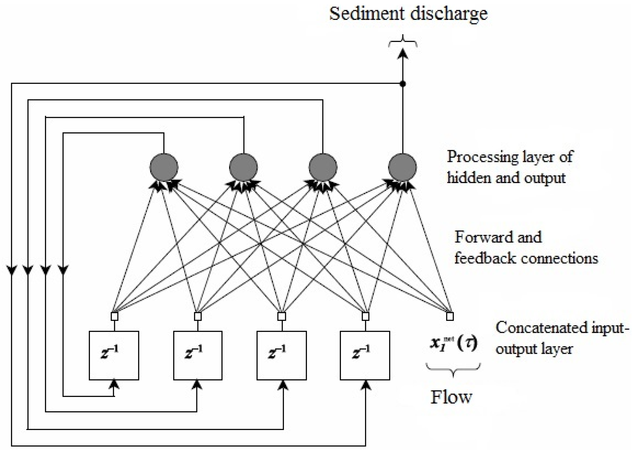
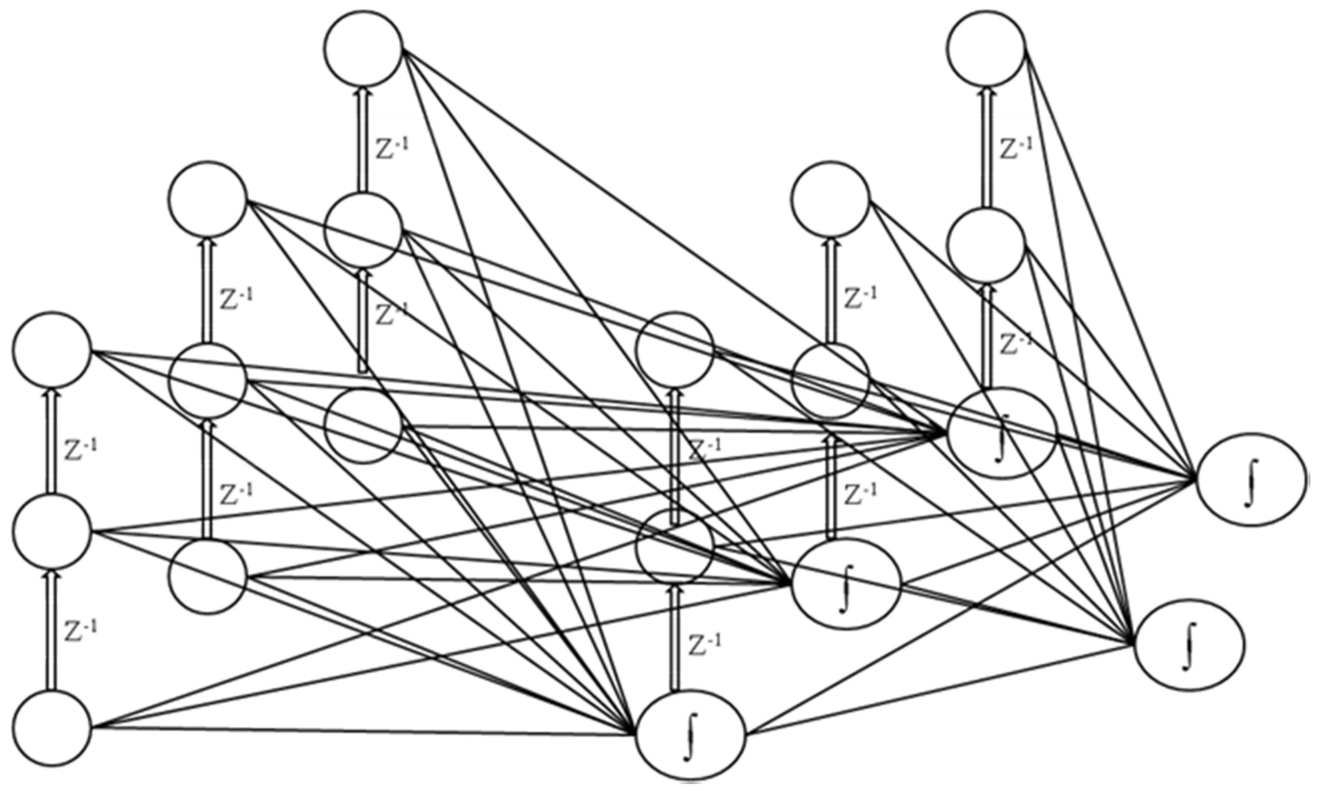
2.3.1. Fully Recurrent Neural Networks (FRNNs)

Recurrent neural networks (Figure 3) are composed of at least one feedback connection at which the output is fed back to inputs such that activation flows in a loop. This is contrary to feed forward neural networks, in which there are no loops and outputs are associated only with inputs of elements in successive layers. According to Martens and Sutskever [15], these types of neural networks can store information about time, making them appropriate for predicting applications. They have been successfully applied in several time series experiments. The architectures of FRNN are not limited to form; however, they all possess two similar characteristics: They integrate some elements of multilayer perceptron (MLP) and exploit the powerful non-linear representation capabilities of the MLP.

Similar to the human brain, ANNs learn to accomplish tasks by learning with examples (of input configurations) and will adjust weights on the connections between network nodes. There are numerous learning algorithms that are available for use to compute the required weight changes [9,16]. In the present study, to train the fully recurrent network, we adopted back-propagation through time. This technique is founded on changing the FRNN from a feedback system to a feed-forward system by collapsing the network with time [17]. Further, the FRNN was based on TahnAxon and momentum algorithms.

Figure 3. Architecture of the FRNN model.

Figure 3. Architecture of the FRNN model.

Several combinations of the different core parameters, like number of processing elements (neurons), hidden layers and data segregation methods, were tried. Based on observations made by [18,19] that one hidden layer is enough for ANNs to estimate any complex non-linear function, we used one hidden layer. The general architecture of the FRNN model used is shown in Figure 3, in which there is 1 input (flow) and 1 output (in our case being sediment discharge) and a hidden layer possessing 4 processing elements. In our study, processing elements were varied between 1 and 12 and the best combination was selected guided by the lowest root mean square error (RMSE) and higher coefficients of determination scores. The conditions for training the FRNN model are shown in Table 1. In total, there were 170 patterns of data from which 60% were used for training, 20% for cross validation and 20% for testing. The training dataset was used to train the neural network by minimizing errors. Cross validation data were used to determine the FRNN performance by regulating the training process. Finally, we evaluated the overall performance by using the test data.

Table 1. Configurations of FRNN during training.

Training Variables	Assigned Value
Step size	1
Momentum	0.7
Iterations	1000
Training threshold	0.001

Table 1. Configurations of FRNN during training.

Training Variables	Assigned Value
Step size	1
Momentum	0.7
Iterations	1000
Training threshold	0.001

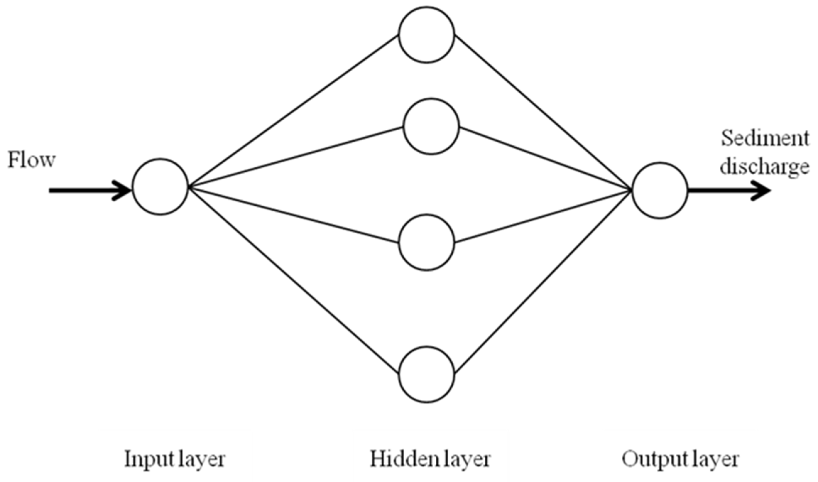
2.3.2. Multilayer Perceptron (MLP)

MLP is characterized by having either one or more hidden layers with hidden neurons, whose purpose is to enhance the relationship between specific inputs and the desired outputs. With additional hidden layers, the computational power of the neural network in terms of statistics is greatly enhanced. Despite this capabaility with increased hidden layers, several researchers have proven otherwise. They have demonstrated that one hidden layer is enough for a neural network to estimate any complex non-linear model/function [18]. Henceforth, we adopted a single hidden MLP layer in this study.

As stated earlier, neural networks require training. MLP is trained by several backpropagation algorithms. The overall function of training is to adjust the connecting weights accordingly in order to attain higher accuracies in the desired output. At each connection weight configuration, errors and accuracies can be determined by comparing the desired outputs to actual outputs [20,21]. In this study, we use the momentum algorithm of the six available learning algorithms. Selection was based on the algorithm that trained the network efficiently. The TahnAxon activation function was preferred as the activation function of the model by the virtue of being successful in interrelating the input and output parameters based on [22]. Throughout all the simulations, we used a trial and error method to determine appropriate hidden layer neurons (PE) for predicting sediments. The processing elements were varied from 1 to 12. In total, there were 170 patterns of data from which 60%, 20% and 20% were used for training, cross validation and testing, respectively.

Table 2 shows the condition of the training performance variables for the MLP and Figure 4 shows the developed MLP architecture with a single input of water discharge from which sediment discharge is estimated.

Table 2. Configurations of MLP during training.

Training Variables	Assigned Value
Step size	1
Momentum	0.7
Iterations	5000
Training threshold	0.001

Table 2. Configurations of MLP during training.

Training Variables	Assigned Value
Step size	1
Momentum	0.7
Iterations	5000
Training threshold	0.001

Figure 4. Architecture of the MLP model.

Figure 4. Architecture of the MLP model.

2.3.3. Time Lagged Recurrent Networks (TLRNs)

TLRNs are multilayer perceptrons (MLP) networks having their memory layer cramped to inputs. This feature makes them best suited for time varying information. They have one main advantage over MLPs; they require a small network size to learn temporal problems [23]. Further, they are less sensitive to noise. The architecture of this network generally has 3 layers (input, hidden layer and output) and a feedback connection from the hidden layer back to the input layer. TLRN provides a number of memory structures at the input layer to choose from, but in this study we used the Laguerre function as shown in Equation (1), (m is the memory resolution and z⁻¹ denotes the delay operator and i is 1, 2, 3…).

$$L_i\left(z,m\right)=\sqrt{1-{\left(1-m\right)}^2}\frac{{\left(z^{-1}-\left(1-m\right)\right)}^{i-1}}{{\left(1-\left(1-m\right)z^{-1}\right)}^i}$$

(1)

We adopted the momentum setup as a learning rule for each layer, with the TanhAxon used as an activation function. Processing elements and epochs were obtained through trial and error. A summary of the conditions under which performance variables for the TLRN are trained is presented in Table 3 and Figure 5 shows a typical structure of the TLRN model.

Table 3. Configurations of TLRN during training.

Training Variables	Assigned Value
Depth in samples	10
Trajectory length	50
Momentum	0.7
Iterations	1000
Training threshold	0.001

Table 3. Configurations of TLRN during training.

Training Variables	Assigned Value
Depth in samples	10
Trajectory length	50
Momentum	0.7
Iterations	1000
Training threshold	0.001

Figure 5. Architecture of the TLRN model.

Figure 5. Architecture of the TLRN model.

2.3.4. Radial Basis Function (RBF)

RBF networks are 2-layer feedforward neural networks whose main application is in supervised learning. The RBF adopts Gaussian transfer functions, instead of the typical sigmoidal functions used by MLPs and combines the advantage of generality and reduced computational complexity [24]. Unsupervised technique rules (called k-nearest neighbour rule) are responsible for adjusting the Gaussians widths and centers, after which supervised learning is utilized in the output layer. In principle, the radial basis functions architecture is similar to that of multilayer perceptron (Figure 4). They have an input layer that receives signals and transfers them to hidden layer(s); these in turn, performs non-linear computations. Finally, there is a linear output layer that supplies the results of the network. RBF’s good estimation probabilities have been studied in [25]. Due to their non-linear approximating probabilities, they are able to model complex mappings. Tabari et al. [26] likens RBF learning to finding an optimum surface in a multifaceted space. Basically, the optimum surface can be found using three metric functions in the RBF model (Box Car, Dot product and Euclidean) and in this study we used the Euclidean metric function. The Euclidean distance, ${\mathsf{\phi }}_j$, between the input x_i and the connection weight, w_j, can be computed by Equation (2) [25].

$${\mathsf{\phi }}_j\left(x_i\right)=\mathsf{\Phi }\left(\frac{\left|\right|x_i-w_j\left|\right|}{{\mathsf{\sigma }}_j}\right)$$

(2)

where Ф, a radial basis function, which is assumed to be a Gaussian exponential, is obtained by computing vector w_j, for the jth hidden unit, the Gaussian basis function smoothing parameter for the j neuron is denoted by σ_j. Finally, a linear output will yield RBF as:

$$y_k={\displaystyle \sum }_{j=1}^h{w}_{kj}{\mathsf{\phi }}_j\left(x_i\right)=W_k^T\mathsf{\phi }$$

(3)

where y_k is a linearly weighted sum of the outputs of the hidden units, $W_k^T$ is the weight vector for the output neuron k and φ is the vector of outputs from the hidden layer; T indicates the transpose operation. Conditions of the training performance variables of the RBF were similar to those of MLP above (Table 2).

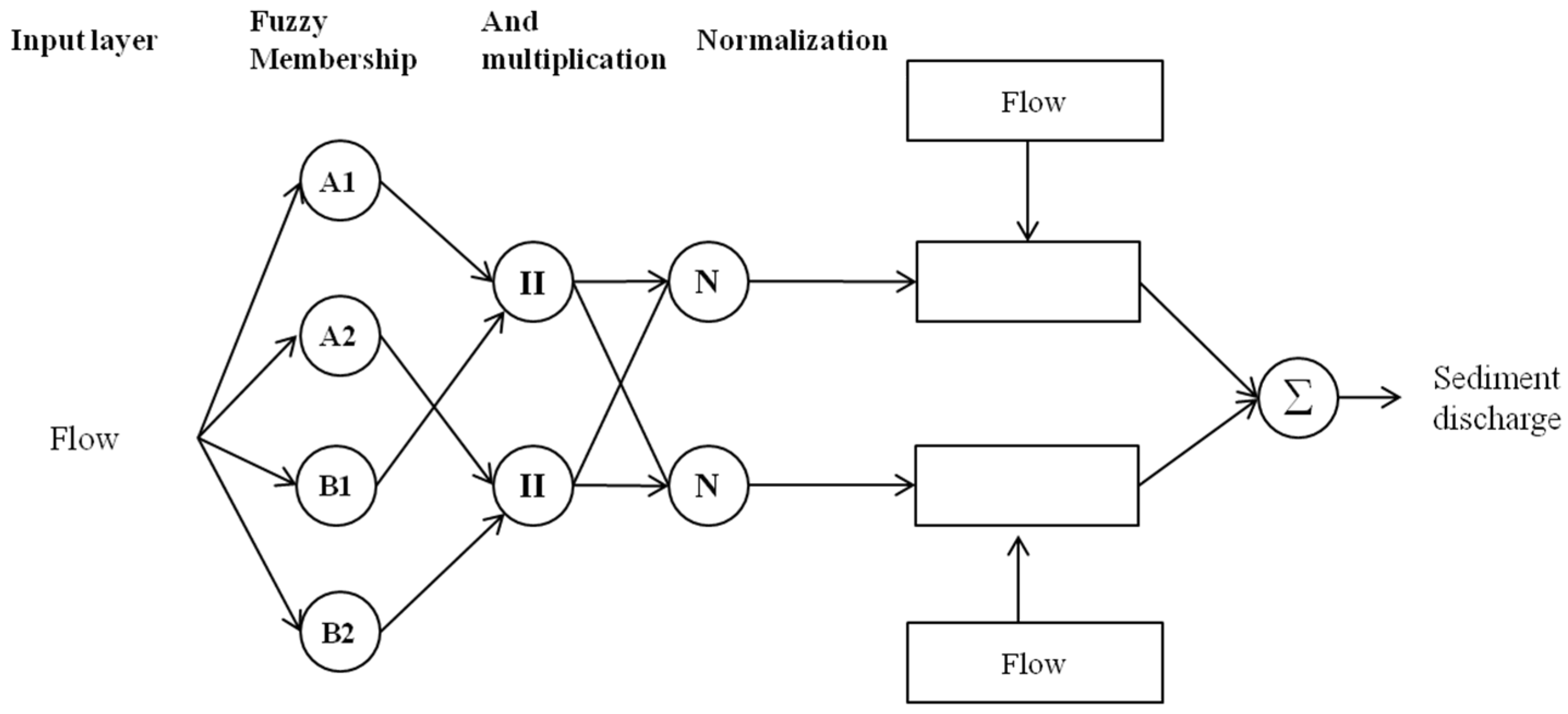
2.3.5. Coactive Neurofuzzy Inference System Model (CANFISM)

The coactive neurofuzzy inference system model (CANFISM) is housed in the adaptive neuro-fuzzy inference model (ANFISM). In ANFISM, directional links connect the several nodes making up the model. Each node is characterized by a node function with fixed or adjustable parameters. It may be used as a universal approximator of any non-linear function [26]. In addition, it mixes adjustable fuzzy inputs with a modular neural network to precisely compute complex functions. CANFISM has added advantages in that it can integrate the same topology neural networks and fuzzy inference. Pattern-dependant weights between the consequent layer and the fuzzy association layer is the key feature of CANFISM models [27]. Fuzzy inference systems are also valuable since they combine membership functions with the power of “black box” neural networks. Gaussian and bell are the frequently applied membership functions. In this study we employed the Gaussian fuzzy axon type. The advantage of this function is that the fuzzy synapses help in characterizing inputs that are not easily discretized [26]. A modular network applying effective rules to the inputs is an additional strength of this kind of CANFISM. The modular network number corresponds to network output number and the processing elements of each network are the same as the membership functions. Table 4 below shows the configurations adopted for the CANFISM model.

Table 4. Configurations of CANFISM during training.

Training Variables	Assigned Value
Membership function	Gaussian
MFs per input	2
Fuzzy model	TSK
Step size	1
Momentum	0.7
Iterations	1000
Training threshold	0.001

Table 4. Configurations of CANFISM during training.

Training Variables	Assigned Value
Membership function	Gaussian
MFs per input	2
Fuzzy model	TSK
Step size	1
Momentum	0.7
Iterations	1000
Training threshold	0.001

In this study, the CANFISM architecture used had one input and one output. The hourly flow data manually observed at Shiwen were used as inputs to the model and sediment discharge was our desired output (Figure 6). From the 170 patterns of data, 60%, 20% and the remaining 20% were adopted for training, cross validation and testing of the CANFISM model, respectively. Membership functions to be assigned in each network input were alternated between 1 and 12 and the best was selected on the basis of correlation coefficients. From the different methods within the CANFISM network (Quickprop, Step, Levenberg-Marquardt, Momentum, Delta-Bar-Delta and ConjugateGradient), we used the momentum. Besides, there are several transfer functions, which include Tanh, Linear Sigmoid, Bias, Sigmoid, Linear and Linear Tanh that were tried to determine one that would give the best estimations of sediments in the studied river. From these, we selected the TanhAxon transfer function. The best network architecture for each function was determined by trial and error and was selected based on minimum errors and maximum coefficients of determination criteron.

Figure 6. Architecture of the CANFISM model.

Figure 6. Architecture of the CANFISM model.

2.4. Data Normalization

Prior to any statistical procedures, data are usually processed to filter out outliers and extreme values, fill in missing values, etc. Similarly, before using the flow data in our neural network models, data were processed following Equation (4) [8,28] and were scaled in the 0 to 1 range. To eliminate biases, we further randomized the flow data before splitting them into the different group sets, i.e., training, cross validation and testing groups.

$$X_{norm}=\frac{X_i-X_{min}}{X_{max}-X_{min}}$$

(4)

where $X_{norm}$ is the scaled input value, $X_i$ is the actual unscaled observed discharge input; $X_{min}$ and $X_{max}$ refer to the minimum and maximum values of the flow data, respectively.

2.5. Models Evaluation

The performance of the neural network models applied is assessed using a variety of standard statistical indexes. In our study, we evaluated the models using three indexes; root mean square error (RMSE), mean absolute error (MAE) and coefficient of correlation (R) (Equations (5) to (8)). The RMSE is a measure of the residual variance. MAE measures how close forecasts or predictions are to eventual outcomes. The R is a measure of accuracy of hydrological modeling and is generally used for comparison of alternative models.

$$RMSE=\sqrt{\frac{{{\displaystyle \sum }}_{i=1}^N{\left(y_i-y_i^{\prime }\right)}^2}{N}}$$

(5)

$$MAE=\frac{1}{N}{\displaystyle \sum }_{i=1}^N\left|y_i-y_i^{\prime }\right|$$

(6)

$$r=\frac{{{\displaystyle \sum }}_{i=1}^N\left(y_i-\overline{y}\right)\left(y_i^{\prime }-{\overline{y}}^{\prime }\right)}{\sqrt{{{\displaystyle \sum }}_{i=1}^N{\left(y_i-{\overline{y}}^{\prime }\right)}^2{{\displaystyle \sum }}_{i=1}^N{\left(y_i-{\overline{y}}^{\prime }\right)}^2}}$$

(7)

where $y_i$ represents the observed sediment discharge, $y_i^{\prime }$ is the alternative methods-estimated sediment discharge values; $\overline{y}$and ${\overline{y}}^{\prime }$ are the mean values of the equivalent parameter; and $N$ is the number of data under consideration. Furthermore, a linear regression $y= \mathsf{\alpha }1x+\mathsf{\alpha }0$ is used to evaluate the model performance statistically, where $y$ denotes the dependent variable (alternative methods); x represents the independent variable (observed); $\mathsf{\alpha }1$ the slope and $\mathsf{\alpha }0$ the intercept.

3. Results and Discussion

3.1. Sediment Discharge—Based on Rating Curve

The sediment rating curve developed by the Q-Qs relationship for available data at Shiwen is presented in Figure 7. In the discharge (Q)-sediment discharge (Qs) relationship, the SRC yielded an R² of 0.621 as shown in Figure 7a. The best fit power function in Figure 7a shows more variation between the observed and estimated discharge. After using the allocated data set (34) for testing, the observed and estimated R² is 0.765 as seen in Figure 7b.

Figure 7. Scatter plot of (a) relationship between water and sediment discharge, (b) observed and estimated sediment discharge.

Figure 7. Scatter plot of (a) relationship between water and sediment discharge, (b) observed and estimated sediment discharge.

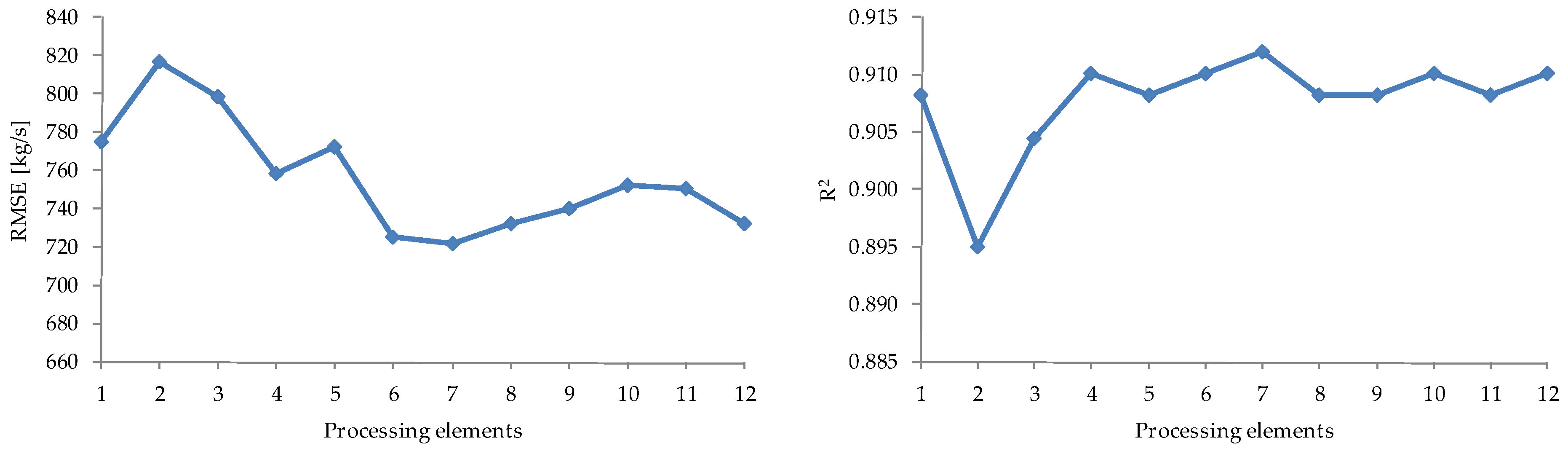
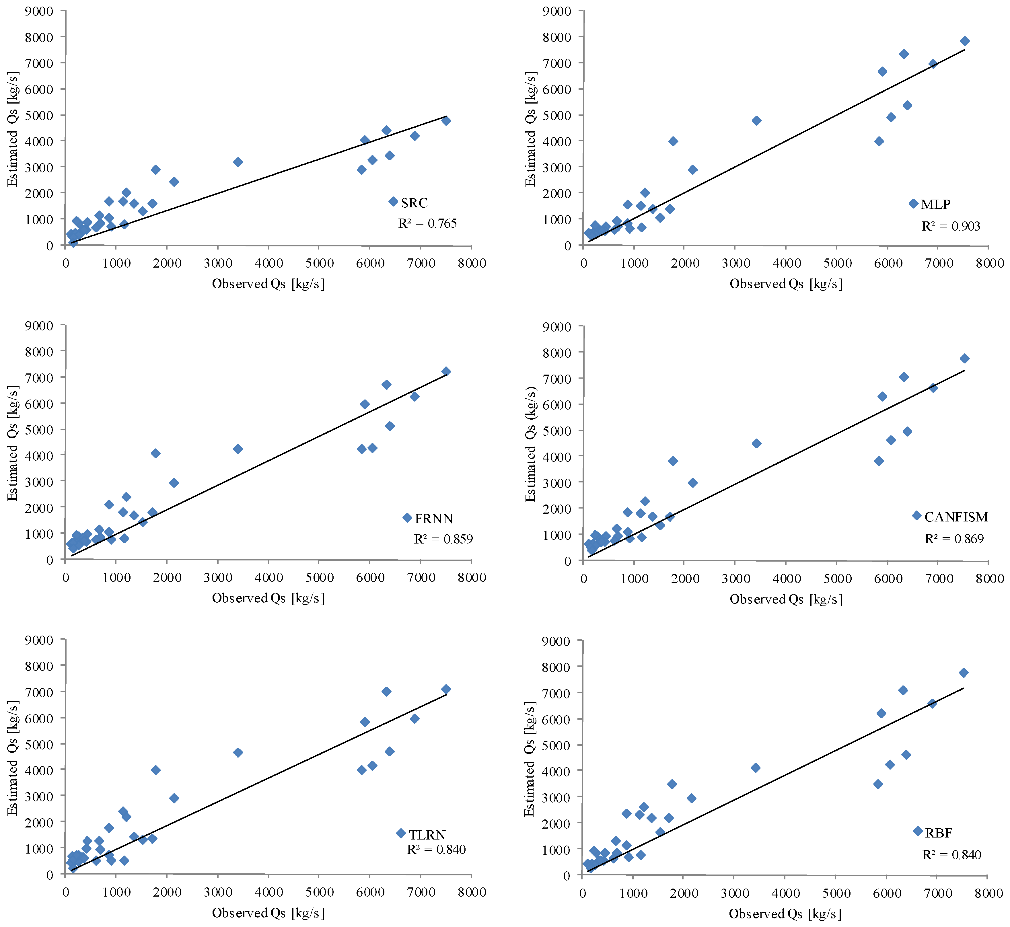
3.2. Sediment Discharge—Based on ANNs

Determining the processing elements (PE) (or membership functions (MF) in the case of CANFISM is a difficult task in neural network models [20]. Despite being a difficult task, it is an essential factor, which may influence the overall neural network performance. Hence, determination of PE/MF was the first process during the learning process for the adopted ANNs. The number of PE/MF was varied between 1 and 12 and the optimum PE was found at 7 for the MLP, which outperformed the other models based on minimum RMSE and maximum R² as shown by Figure 8. A summary of the model’s statistical performance is shown in Table 5. The RMSE values of MLP for training, cross validation and testing stage were 1431.536, 1091.186 and 721.175 kg/s, respectively. The R² values in the training, cross validation and testing stages were 0.709, 0.823 and 0.912, respectively.

Figure 8. MLP accuracy under a different number of processing elements.

Figure 8. MLP accuracy under a different number of processing elements.

Table 5. Summary of model statistical performance.

Model	Stage	RMSE (m3/s)	MAE (m3/s)	R2
MLP	Training	1431.536	893.700	0.709
	Cross validation	1091.186	706.003	0.823
	Testing	721.175	509.584	0.912
CANFISM	Training	1380.483	890.829	0.721
	Cross validation	1122.562	758.043	0.826
	Testing	775.401	591.837	0.906
TLRN	Training	1329.052	900.685	0.743
	Cross validation	1187.290	786.072	0.801
	Testing	860.803	649.805	0.878
FRNN	Training	1400.275	931.110	0.716
	Cross validation	1142.759	775.643	0.823
	Testing	782.847	588.648	0.906
RBF	Training	1359.194	844.964	0.729
	Cross validation	1124.365	730.110	0.828
	Testing	859.805	615.986	0.876

Table 5. Summary of model statistical performance.

Model	Stage	RMSE (m3/s)	MAE (m3/s)	R2
MLP	Training	1431.536	893.700	0.709
	Cross validation	1091.186	706.003	0.823
	Testing	721.175	509.584	0.912
CANFISM	Training	1380.483	890.829	0.721
	Cross validation	1122.562	758.043	0.826
	Testing	775.401	591.837	0.906
TLRN	Training	1329.052	900.685	0.743
	Cross validation	1187.290	786.072	0.801
	Testing	860.803	649.805	0.878
FRNN	Training	1400.275	931.110	0.716
	Cross validation	1142.759	775.643	0.823
	Testing	782.847	588.648	0.906
RBF	Training	1359.194	844.964	0.729
	Cross validation	1124.365	730.110	0.828
	Testing	859.805	615.986	0.876

Figure 9, Figure 10 and Figure 11 presents the observed and the estimated sediment discharge for training, validation, and testing stages for the MLP model, respectively. From the figures it can be seen that the patterns of predicted sediment data are almost similar to observed data in all stages (training, cross validation and testing). At the intial stage, i.e., training, MLP seem to have overestimated sediment discharge for smaller peaks as seen during the 5th, 18th, 27th hour, etc. During cross validation, MLP underestimated sediment discharge around the 6th hour. Finally, at the final stage (testing), there is not much variation between the observed and the predicted sediment discharge. The corresponding scatter for the testing stage (MLP) is shown in Figure 12 together with all the adopted models.

Figure 9. Observed and estimated sediment discharge at training stage using MLP.

Figure 9. Observed and estimated sediment discharge at training stage using MLP.

Figure 10. Observed and estimated sediment discharge at cross validation stage using MLP.

Figure 10. Observed and estimated sediment discharge at cross validation stage using MLP.

Figure 11. Observed and estimated sediment discharge at testing stage using MLP.

Figure 11. Observed and estimated sediment discharge at testing stage using MLP.

Figure 12. Scatter plots of observed and estimated discharge using the five ANNs compared to SRC.

Figure 12. Scatter plots of observed and estimated discharge using the five ANNs compared to SRC.

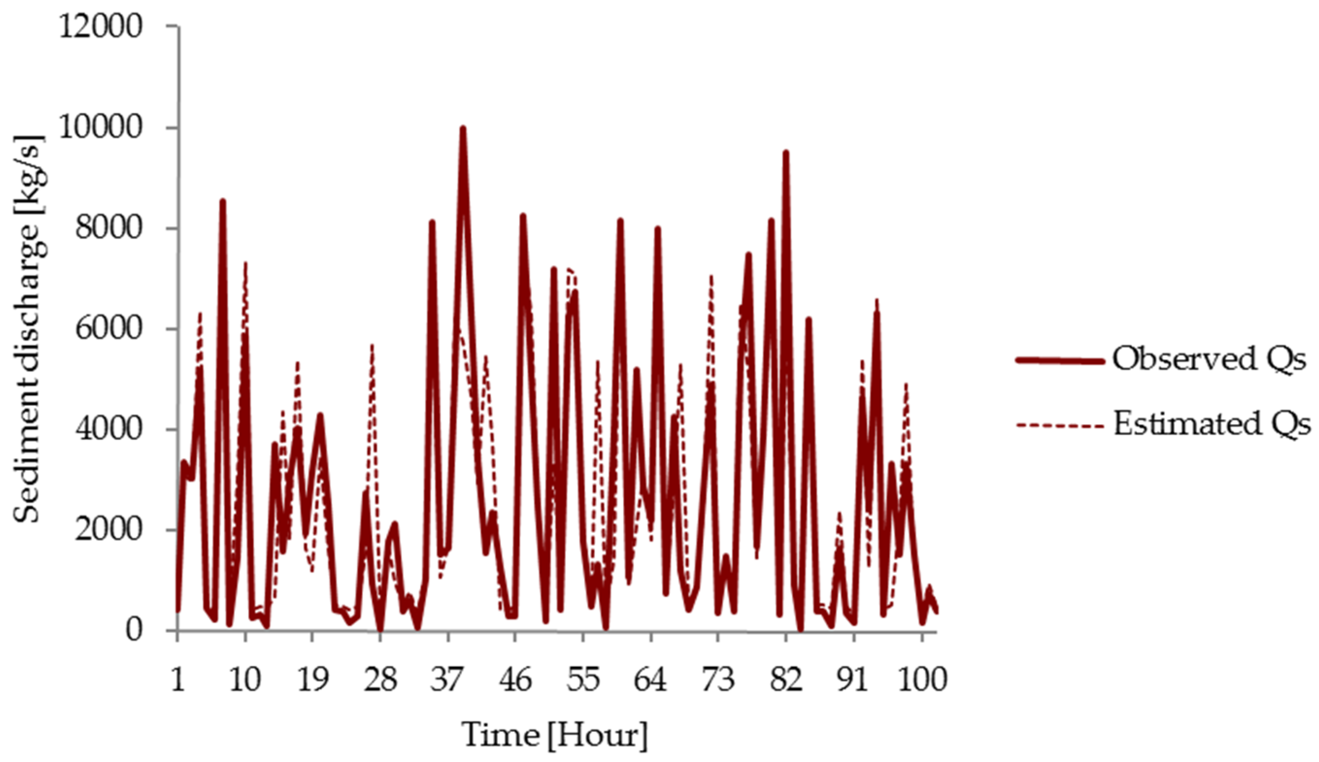
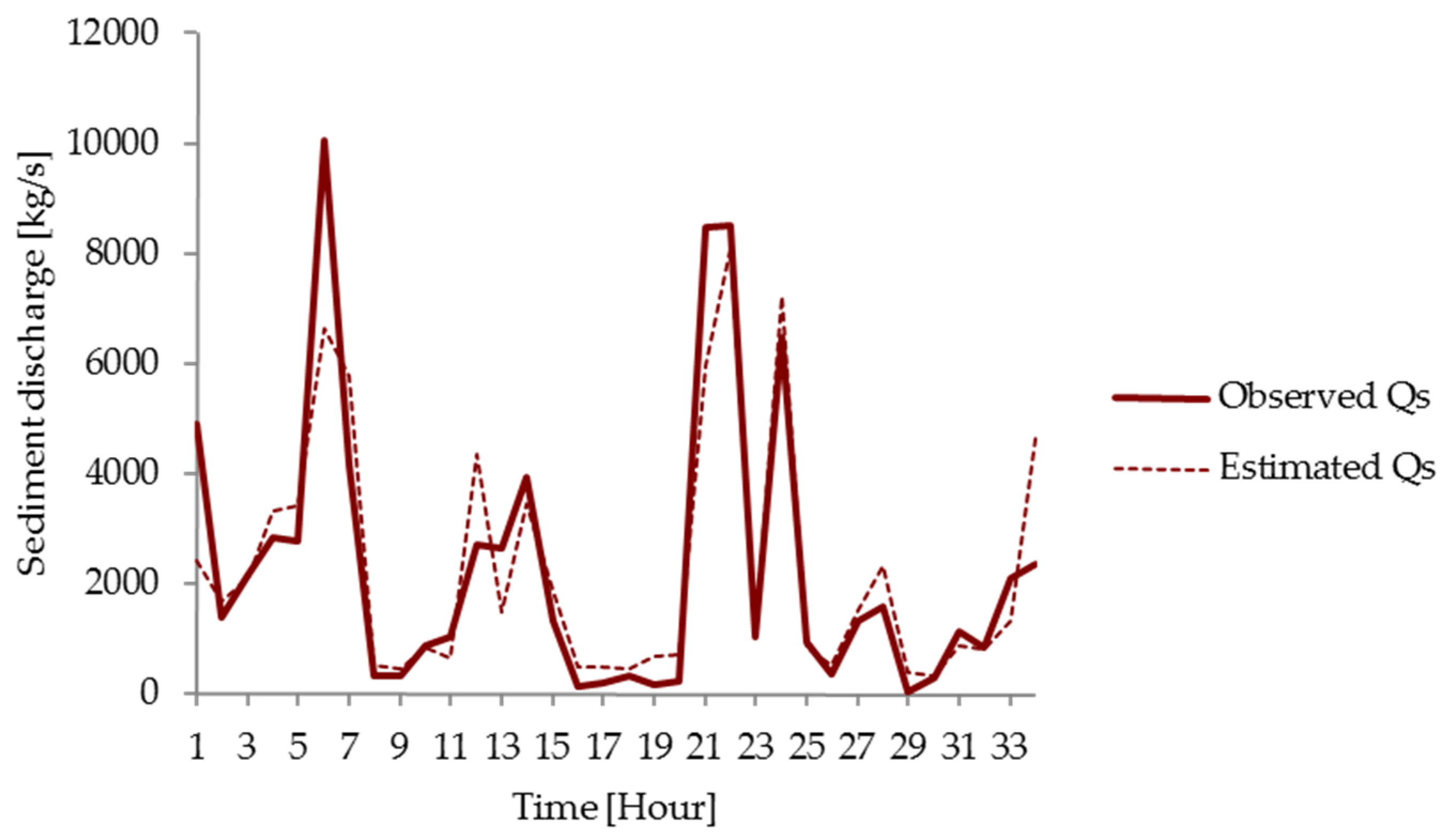
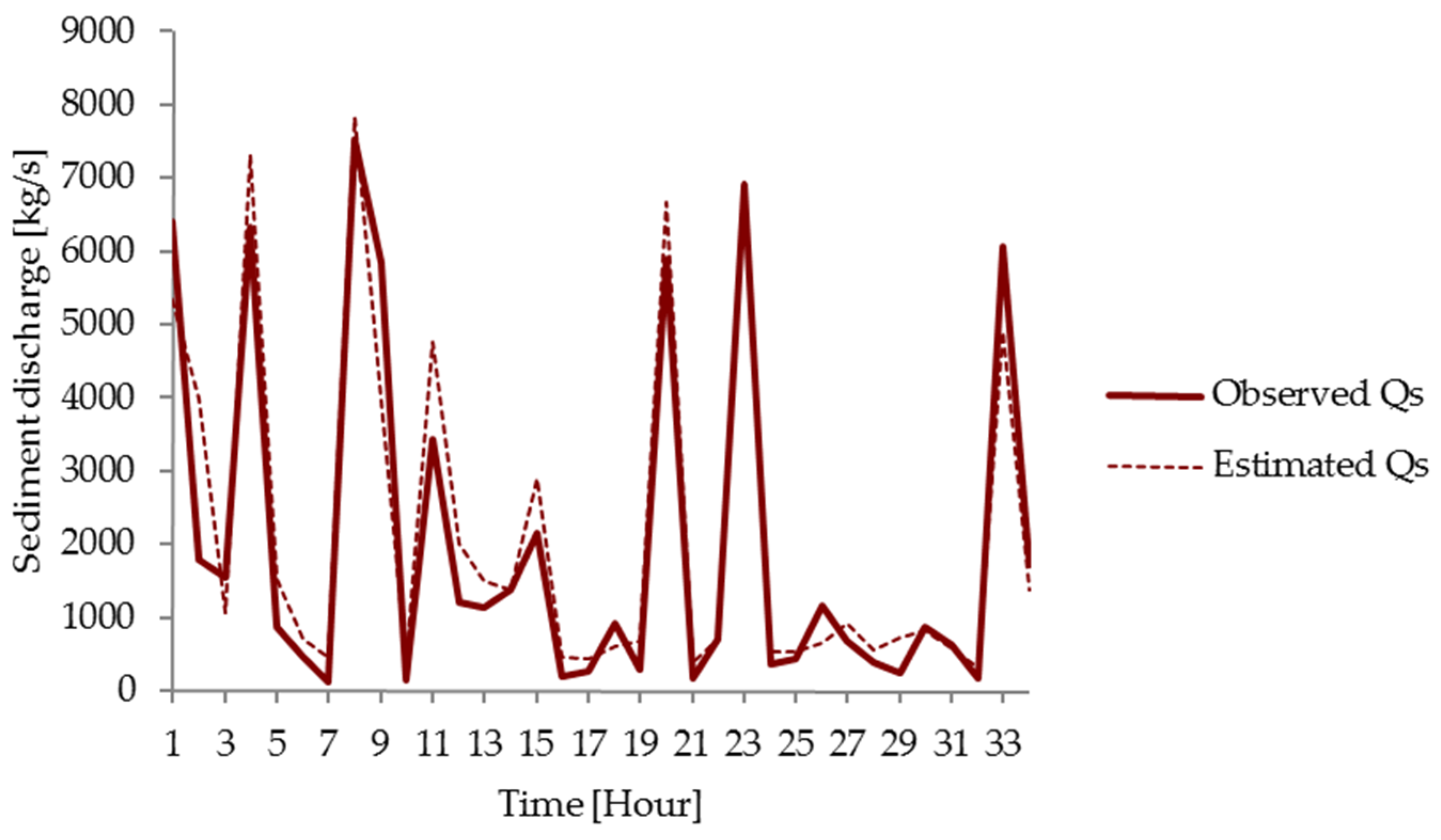
3.3. Comparison of Models

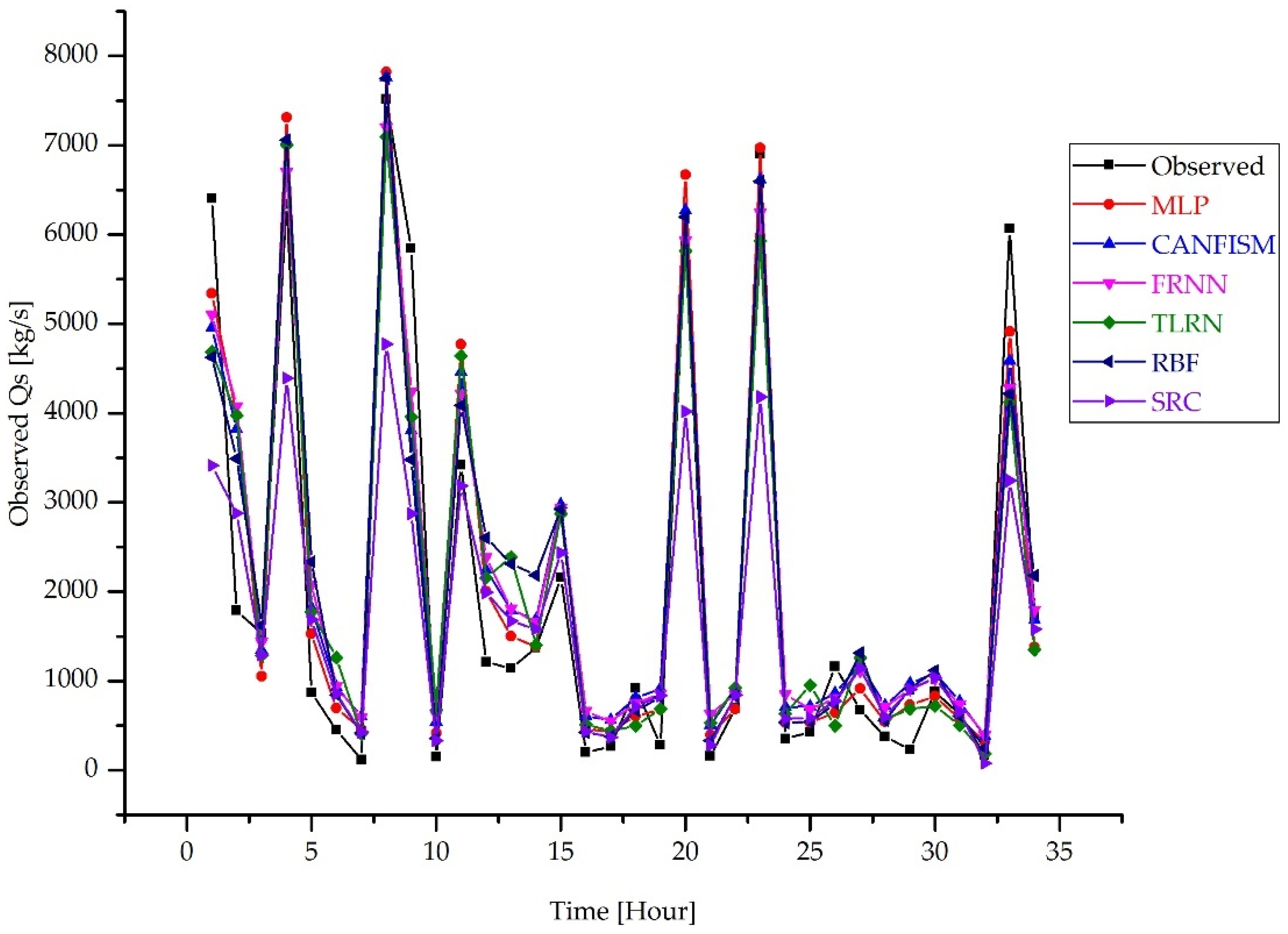
An effort was made to compare SRC and ANN for predicting sediment discharge during storm events. To enable comparison, the 170 data sets were divided into 2 and 3 for multiple linear regressions and ANNs, respectively. We used twenty percent (34 data sets) of the available data for testing and comparing all the used models. The same data used to test the multiple linear regressions for SRC are used to test the developed ANNs. From the evaluation of these results, ANNs are superior to conventional methods in estimating sediment discharge. The developed SRC yielded an R² of 0.621 (Figure 7); however, during testing, the R² shoots up to 0.765 to an almost similar R² for the ANN models as seen in Figure 12. Moreover, Figure 13 shows that the high SRC R² obtained during the testing stage may be misleading as it underestimated sediment discharge especially at the peaks and overestimated low sediment discharge values when compared with observed Qs. The observed and estimated peak Qs are shown in Table 6. The ANNs (MLP and FRNN = 1%), model peak Qs values are almost similar to the observed values compared to the developed sediment rating curve (−47%). Lin [28] observed that SRC can underestimate sediment load by as much as −73% and can overestimate by as high as 224%. These findings demonstrate the inappropriateness of employing linear models in solving non-linear and complex hydrological systems like that of Taiwan. Leahy et al. [14] concluded that river studies are necessary but are a challenging mission because their hydrologic systems are very complex. Boukhrissa et al. [29] compared a feed forward back propagation (FFBP) neural network with sediment rating curves, and the FFBP model results showed high efficiencies in reproducing daily sediment loads and global annual sediment yields.

Figure 13. Observed and estimated sediment discharge during the testing stage.

Figure 13. Observed and estimated sediment discharge during the testing stage.

Table 6. The comparison of peak estimations of the different models in the test phase.

Observed	MLP	CANFISM	FRNN	TLRN	RBF	SRC	Relative Error (%)
(Kg/s)							MLP	CANFISM	FRNN	TLRN	RBF	SRC
6402	5341	4954	5104	4689	4625	3414	−17	−23	−20	−27	−28	−47
6339	7312	7046	6701	7002	7062	4392	15	11	6	10	11	−31
7520	7822	7760	7202	7095	7749	4775	4	3	−4	−6	3	−37
3418	4768	4461	4218	4641	4087	3186	39	31	23	36	20	−7
2160	2901	2977	2932	2872	2923	2437	34	38	36	33	35	13
5904	6671	6271	5936	5815	6197	4017	13	6	1	-2	5	−32
6904	6969	6616	6243	5927	6595	4180	1	−4	−10	−14	−4	−39
6065	4915	4584	4280	4123	4216	3244	−19	−24	−29	−32	−30	−47

Table 6. The comparison of peak estimations of the different models in the test phase.

Observed	MLP	CANFISM	FRNN	TLRN	RBF	SRC	Relative Error (%)
(Kg/s)							MLP	CANFISM	FRNN	TLRN	RBF	SRC
6402	5341	4954	5104	4689	4625	3414	−17	−23	−20	−27	−28	−47
6339	7312	7046	6701	7002	7062	4392	15	11	6	10	11	−31
7520	7822	7760	7202	7095	7749	4775	4	3	−4	−6	3	−37
3418	4768	4461	4218	4641	4087	3186	39	31	23	36	20	−7
2160	2901	2977	2932	2872	2923	2437	34	38	36	33	35	13
5904	6671	6271	5936	5815	6197	4017	13	6	1	-2	5	−32
6904	6969	6616	6243	5927	6595	4180	1	−4	−10	−14	−4	−39
6065	4915	4584	4280	4123	4216	3244	−19	−24	−29	−32	−30	−47

4. Conclusions

Correct estimation of sediment discharge and consequently, sediment load is an essential component in river management. The key objective of this study was to evaluate the accuracy of artificial neural networks in estimating sediment discharge in rivers during storm events. Data collected during 8 typhoon events were used to establish a sediment rating curve and also acted as inputs to the ANNs (MLP, CANFISM, TLRN, FRNN and RBF). Comparison of peak Qs estimates revealed that SRC can underestimate Qs by as much as −47%, hence, compromising water management projects. The study further shows that artificial neural networks can be successfully adopted in this typhoon-prone region to aid in the precise estimations of sediment movement. Among the 5 ANN models, MLP performed best overall with an R² of 0.903 obtained during application. Finally, the inaccuracies associated with using SRC in estimating sediment loads and discharge can be overcome by employing articial neural networks. Different catchments are likely to have different outcomes from our findings; however, extensive data collection during storm events before applying the outlined methodologies is recommended for better results.

References

1. Chen, S.L.; Zhang, G.A.; Young, S.L.; Shi, J.Z. Temporal variations of fine suspended sediment concentration in the Changjiang River estuary and adjacent coastal waters, China. J. Hydrol. 2006, 331, 137–145. [Google Scholar] [CrossRef]
2. Wang, Y.M.; Tfwala, S.S.; Chan, H.C.; Lin, Y.C. The effects of sporadic torrential rainfall events on suspended sediments. Arch. Sci. J. 2013, 66, 211–224. [Google Scholar]
3. Teng, W.-H.; Hsu, M.-H.; Wu, C.-H.; Chen, A.S. Impact of flood disasters on taiwan in the last quarter century. Nat. Hazards 2006, 37, 191–207. [Google Scholar] [CrossRef] [Green Version]
4. Milliman, J.D.; Syvitski, J.P. Geomorphic/tectonic control of sediment discharge to the ocean: The importance of small mountainous rivers. J. Geol. 1992, 525–544. [Google Scholar] [CrossRef]
5. Horowitz, A.J. An evaluation of sediment rating curves for estimating suspended sediment concentrations for subsequent flux calculations. Hydrol. Process. 2003, 17, 3387–3409. [Google Scholar] [CrossRef]
6. Thomas, R.B. Estimating total suspended sediment yield with probability sampling. Water Resour. Res. 1985, 21, 1381–1388. [Google Scholar] [CrossRef]
7. Wang, Y.M.; Traore, S. Time-lagged recurrent network for forecasting episodic event suspended sediment load in typhoon prone area. Int. J. Phys. Sci. 2009, 4, 519–528. [Google Scholar]
8. Chen, S.M.; Wang, Y.M.; Tsou, I. Using artificial neural network approach for modelling rainfall–runoff due to typhoon. J. Earth Syst. Sci. 2013, 122, 399–405. [Google Scholar] [CrossRef]
9. Tfwala, S.S.; Wang, Y.M.; Lin, Y.C. Prediction of missing flow records using multilayer perceptron and coactive neurofuzzy inference system. Sci. World J. 2013, 2013, 584516. [Google Scholar] [CrossRef] [PubMed]
10. Melesse, A.M.; Ahmad, S.; McClain, M.E.; Wang, X.; Lim, Y.H. Suspended sediment load prediction of river systems: An artificial neural network approach. Agric. Water Manag. 2011, 98, 855–866. [Google Scholar] [CrossRef]
11. Kisi, O. Generalized regression neural networks for evapotranspiration modelling. Hydrol. Sci. J. 2006, 51, 1092–1105. [Google Scholar] [CrossRef]
12. Wang, Y.M.; Traore, S.; Kerh, T. Computing and modelling for crop yields in burkina faso based on climatic data information. WSEAS Trans. Inf. Sci. Appl. 2008, 5, 832–842. [Google Scholar]
13. Lin, J.Y.; Cheng, C.T.; Chau, K.W. Using support vector machines for long-term discharge prediction. Hydrol. Sci. J. 2006, 51, 599–612. [Google Scholar] [CrossRef]
14. Leahy, P.; Kiely, G.; Corcoran, G. Structural optimisation and input selection of an artificial neural network for river level prediction. J. Hydrol. 2008, 355, 192–201. [Google Scholar] [CrossRef]
15. Martens, J.; Sutskever, I. Learning recurrent neural networks with hessian free optimization. In Proceedings of the 28th International Conference on Machine Learning, Belluvue, WA, USA, 28 June–2 July 2011.
16. Wang, Y.M.; Kerh, T.; Traore, S. Neural network approach for modelling river suspended sediment concentration due to tropical storms. Glob. NEST J. 2009, 11, 457–466. [Google Scholar]
17. Maraqa, M.; Abu-Zaiter, R. Recognition of Arabic Sign Language (ArSL) using recurrent neural networks. In Proceedings of the First International Conference on the Applications of Digital Information and Web Technologies, 2008—ICADIWT 2008, 4–6 August 2008; pp. 478–481.
18. Feyzolahpour, M. Estimating suspended sediment concentration using neural differential evolution (NDE), multi layer perceptron (MLP) and radial basis function (RBF) models. Int. J. Phys. Sci. 2012, 7, 5106–5177. [Google Scholar] [CrossRef]
19. Wang, Y.M.; Traore, S.; Kerh, T.; Leu, J.-M. Modelling reference evapotranspiration using feed forward backpropagation algorithm in arid regions of Africa. Irrig. Drain. 2011, 60, 404–417. [Google Scholar] [CrossRef]
20. Kim, S.; Park, K.B.; Seo, Y.M. Estimation of pan evaporation using neural networks and climate-based models. Disaster Adv. 2012, 5, 34–43. [Google Scholar]
21. Suditu, G.D.; Piuleac, C.G.; Bulgariu, L.; Curteanu, S. Application of a neuro-genetic technique in the optimization of heavy metals removal from wastewaters for environmental risk reduction. Environ. Eng. Manag. J. 2013, 12, 167–174. [Google Scholar]
22. Charaniya, N.A.; Dudul, S.V. Time lag recurrent neural network model for rainfall prediction using El Niño indices. Int. J. Sci. Res. Publ. 2013, 3, 1–5. [Google Scholar]
23. Specht, D.F. A general regression neural network. IEEE Trans. Neural Netw. 1991, 2, 568–576. [Google Scholar] [CrossRef] [PubMed]
24. Park, J.; Sandberg, I. Universal approximation using radial-basis-function networks. Neural Comput. 1991, 3, 246–257. [Google Scholar] [CrossRef]
25. Coulibaly, P.; Evora, N.D. Comparison of neural network methods for infilling missing daily weather records. J. Hydrol. 2007, 341, 27–41. [Google Scholar] [CrossRef]
26. Tabari, H.; Talaee, P.H.; Abghari, H. Utility of coactive neuro-fuzzy inference system for pan evaporation modeling in comparison with multilayer perceptron. Meteorol. Atmos. Phys. 2012, 116, 147–154. [Google Scholar] [CrossRef]
27. Wang, Y.M.; Lin, C.P.; Tfwala, S.S.; Chen, C.N.; Chi, T.H. Predicting airport visibility using back propagation neural network. Jokull 2014, 64, 77–90. [Google Scholar]
28. Lin, C.C. Partitioning capabilities of multilayer perceptions on nested rectangular decision regions part I: Algorithm. WSEAS Trans. Inf. Sci. Appl. 2006, 3, 1674–1681. [Google Scholar]
29. Boukhrissa, Z.A.; Khanchoul, K.; Le Bissonnais, Y.; Tourki, M. Prediction of sediment load by sediment rating curve and neural network (ANN) in El Kebir catchment, Algeria. J. Earth Syst. Sci. 2013, 122, 1303–1312. [Google Scholar] [CrossRef]