Article

Analysis of Influencing Factors of Water Footprint Based on the STIRPAT Model: Evidence from the Beijing Agricultural Sector

1
College of Environmental Science and Engineering, Beijing Forestry University, Beijing 100083, China
2
Beijing Key Laboratory of Environmental Science and Engineering, School of Materials Science & Engineering, Beijing Institute of Technology, Beijing 100081, China
*
Author to whom correspondence should be addressed.
Water 2016, 8(11), 513; https://doi.org/10.3390/w8110513
Submission received: 17 August 2016 / Revised: 29 October 2016 / Accepted: 1 November 2016 / Published: 5 November 2016
(This article belongs to the Special Issue Water Footprint Assessment)

Abstract

:
Beijing suffers from a severe water shortage. To find the key factors that impact the agricultural water footprint (WF) within Beijing to relieve the pressure on water resources, this study quantifies the agricultural WF within Beijing from 1980 to 2012 and examines the factors of population, urbanization level, GDP per capita, Engel coefficient, and total rural power using an extended stochastic impact by regression on population, affluence and technology (STIRPAT) model. Ridge regression is employed to fit the extended STIRPAT model. The empirical results reveal that the Engel coefficient, which is defined as the total amount of food expenses accounted for the proportion of total personal consumption expenditures, has the largest positive impact on the increase in the agricultural WF, followed by urbanization. In contrast, total rural power, population, and GDP per capita can decrease the agricultural WF. Finally, policy recommendations from technological development, agriculture plantation structure adjustment, and virtual water imports are provided to cope with water shortages.

1. Introduction

Beijing, the capital of China, is suffering from a serious lack of water resources because of its rapid development and dense population [1]. Beijing is located in the north of the North China Plain and covers an area of 16,410.54 km2, of which 2208.56 km2 is arable land. As the most affluent and populous city in China, Beijing has 21.52 million residents, and the city’s GDP reached 2133.1 billion Yuan, accounting for 3.35% of the GDP of the entire country in 2014 [2]. According to the Beijing Water Authority, the per capita water resources in Beijing were 94 m3 in 2014 [3], which is far below the internationally recognized minimum standard of 1000 m3 per year [4].
Water is one of the most important resources and is necessary to maintain the sustainable development of the earth’s ecological environment. Sustainability indicators for any system are essential for decision makers, especially when the earth is facing environmental and social problems [5]. Several indicators have been used in the last few years to present a quantifiable and rational basis by which to measure the efficiency of production processes and to address the sustainable use of ecological assets across the globe, for instance, the ecological footprint, the carbon footprint, and the water footprint [6]. Among these indicators, the water footprint (WF) was originally proposed by Hoekstra (2003) to measure the quantity of water resources required for all the products and services consumed within a certain period of time [
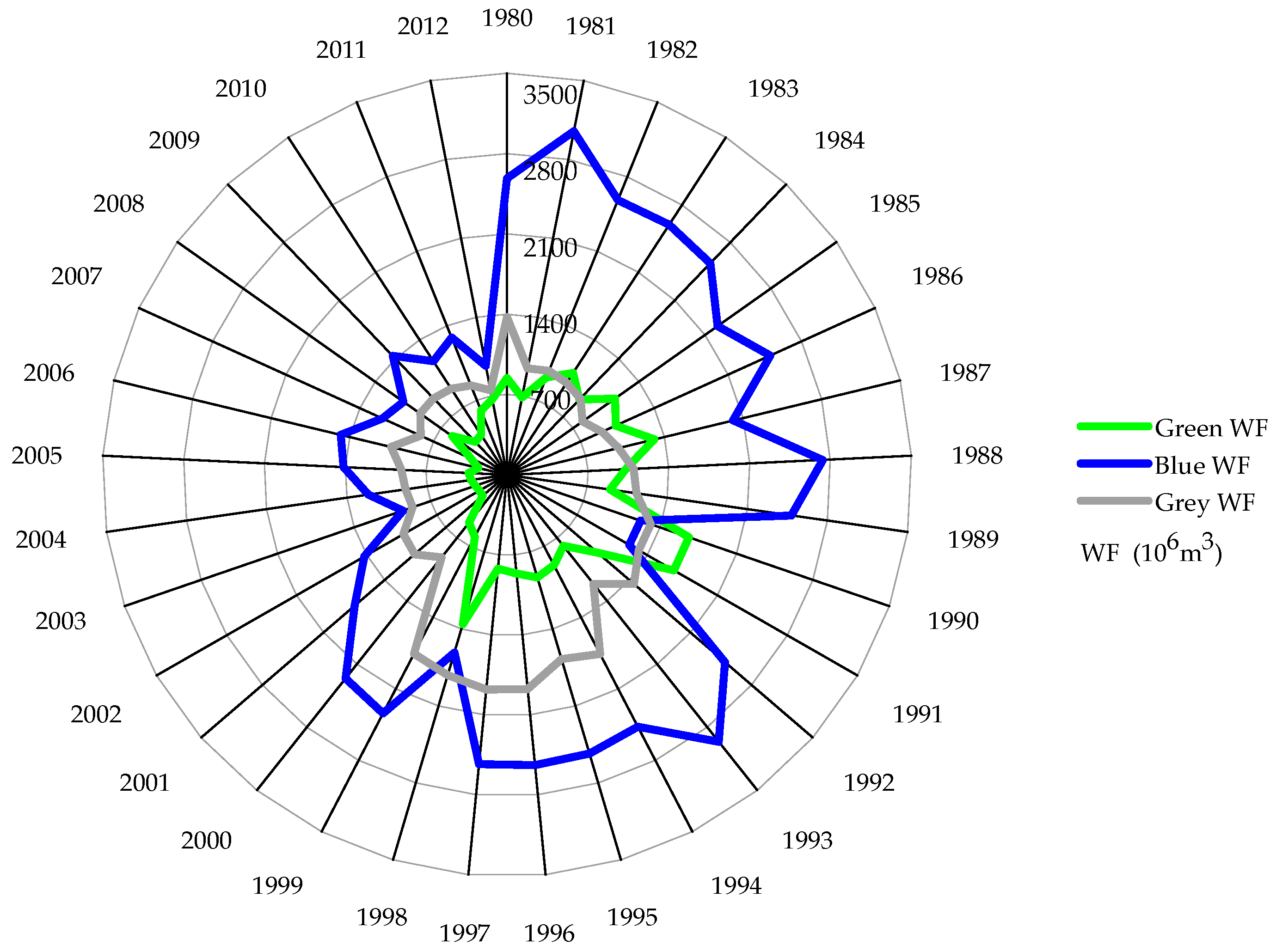
7]. According to the types of water use, the water footprint can be divided into blue water (fresh surface or groundwater), green water (the precipitation on land that does not run off or recharge the groundwater but is stored in the soil or temporarily stays on the top of the soil or vegetation), and grey water (the volume of fresh water that is required to assimilate the load of pollutants based on natural background concentrations and existing ambient water quality standards) [8]. Currently, there are two main WF assessment methods: the Water Footprint Network (WFN) method and the ISO 14046 method, which was developed by the Life Cycle Assessment (LCA) community [9]. Hoekstra believed that the LCA used in the water-scarcity weighted water footprint has some limitations [10]. In contrast, Pfister stressed that the WFN aims to account for the water productivity of global fresh water as a limited resource, while ISO 14046 is concerned with the environment impact [11]. Despite the two communities being somewhat in conflict in the past few years, the two approaches can have the same application [12]. The calculation of the water footprint using the WFN method has been widely used in previous studies at the basin [13], regional [14], national [15], and global scales [16]. For Beijing, Zhang reported the WF of the agriculture in Beijing as 0.667 km3/year in 2002, using an interregional input–output framework [17], and we have also evaluated the gross WF of different sectors in Beijing using an input–output approach [18]. Because this paper aims to account for the water consumed in production processes, we applied the WFN method to quantify the WF.
Agriculture is the largest water use sector in the world, and agricultural production consumes a large proportion of the water resources [19]. The agricultural water consumption of China in 2012 was 3899.443 × 109 m3, accounting for 63.66% of the total water consumption [20]. With the increasing pressure of agricultural water resources, an urgent response is currently needed, and a better understanding of the influence of anthropogenic factors on the environment should be employed. Structural decomposition analysis (SDA) [21], the Logarithmic-Mean Divisia Index (LMDI) [22,23], and stochastic impact by regression on population, affluence, and technology (STIRPAT) [24] are methods that are commonly used to analyze the driving force of changes in the WF. Dietz and Rosa reformulated the IPAT into STIRPAT, which is used to analyze the impact of non-proportional variables on the environment [25,26]. As a stochastic model, the STIRPAT model allows a hypothesis test. In addition, it permits falsifiable tests of the environmental Kuznets curve and modernization theory [27]. This model has simple, systematic, powerful features. It simply includes key anthropogenic driving forces and clarifies the mathematical relationship between the driving forces and their impacts. In addition, it applies to a wide variety of effects [25]. Compared with other decomposition methods, the STIRPAT model is more flexible and easier to operate, while the SDA model needs an input–output table. Moreover, the STIRPAT model can examine more detailed factors than the LMDI, so it can provide more detailed and reliable information [28].
Recently, the STIRPAT model has been extended and applied in several other applications for empirical analyses and policy recommendations [29]. Liddle used the STIRPAT model to study changes in the age structure, urbanization, and climate in developed countries [30], Martínez-Zarzoso analyzed the impact of urbanization on CO2 emissions using the STIRPAT model [31], and Ignatius used the STIRPAT model to examine the impacts of anthropogenic factors on the environment in Nigeria [32]. Our study differs in several ways from previous studies. In particular, the STIRPAT model was widely used to examine the driving factors of CO2 emissions in previous studies, but few works have undertaken a decomposition analysis of the WF [24]. In addition, we make use of this method at the regional scale, which is more targeted. Most importantly, in previous studies, the main drivers of the agricultural WF were the population, GDP, urbanization level, plantation structure, and diet structure. However, these studies ignored the impact of two major transformations that are occurring in Beijing: the constantly increasing standard of living and improvements in cultivation technology. In 2012, the Engel coefficient of Beijing was 31.3%, compared with 55.3% in 1980. In this process, technology develops rapidly. For example, the area of mechanical cultivation as a proportion of the total area of cultivated land has risen from 61% in 2004 to 82.9% in 2012 [33].
In view of these significant changes, this study aims to quantify the influence of anthropogenic factors on the agricultural WF within Beijing by applying the STIRPAT model. First, we calculated the agricultural WF within Beijing from 1980 to 2012. Second, we used a correlation analysis to select the main influencing factors. Finally, we employed an extended STIRPAT model that incorporated ridge regression to decompose and determine the influencing factors. The results of this study provide new insights in the analysis of the anthropogenic driving factors of the agricultural WF within Beijing.

2. Methods and Data

2.1. Water Footprint Evaluation

In this paper, the water footprint of crop production is associated with local crop production and does not include the trade water footprint. The WF is calculated as the total amount of water consumed during the crop growth process and includes the blue WF, the green WF, and the grey WF [34]. We calculated the WF of nine main types of crops planted within Beijing (maize, wheat, vegetables, melons, oil plants, cotton, rice, potato, and soybean), because their total cultivated area accounted for 96.6% of Beijing’s agricultural land area [2].
W F t o t a l = W F g r e e n + W F b l u e + W F g r e y ,
where WFtotal is the total water footprint of crop production in Beijing (m3·year−1), WFgreen is the green water footprint (m3·year−1), which can be estimated with the CropWat model [35], and WFgrey is the grey water footprint (m3·year−1), which refers to the volume of water needed to dilute pollutants to the extent that the quality of ambient water remains above agreed-upon water quality standards.
W F g r e e n = 10 × E T g r e e n × A ,
W F b l u e = 10 × E T b l u e × A ,
where ETgreen and ETblue refer to the quantity of green water evaporation and the quantity of blue water evaporation (mm), respectively, which can be calculated using the CropWat model. The factor 10 is the conversion coefficient, the depth of the water (mm) can be converted to unit land area of water (m3/hm2), and A is the acreage of calculated crops (hm2).
E T g r e e n = m i n ( E T c , P e f f ) ,
E T b l u e = m a x ( 0 , E T c P e f f ) ,
where ETc is crop evapotranspiration during the growth period (mm), and Peff is the effective precipitation over that period (mm). The ETc is calculated using the CropWat model as follows:
E T c = K c × E T 0 ,
where Kc is the crop coefficient and ET0 is the reference crop evapotranspiration (mm), which is calculated according to the FAO Penman–Monteith equation as follows [36]:
E T 0 = 0 . 408 Δ ( R n G ) + γ × 900 T + 273 × u 2 × ( e s e a ) Δ + γ ( 1 + 0 . 34 u 2 ) ,
where Rn represents net radiation at the crop surface (MJ·m−2·day−1); G represents soil heat flux density (MJ·m−2·day−1); γ is the psychrometric constant (kPa·°C−1); T is the average air temperature at a height of 2 m (°C); u2 is the wind speed at a 2 m height (m·s−1); es is the saturation vapor pressure deficit (kPa); ea is the actual vapor pressure (kPa); Δ refers to the slope of the vapor pressure curve (kPa·°C−1).
Peff can be calculated according to the Soil Conservation Service method, which was developed by U.S. Department of Agriculture (USDA):
P e f f { P × ( 125 0 . 6 × P ) / 125 125 / 3 + 0 . 1 × P P ( 250 / 3 ) m m P > ( 250 / 3 ) m m ,
where P is the precipitation (mm).
The grey water footprint of the crop is calculated as follows:
W F g r e y = α × A R ( c m a x c n a t ) × Y ,
where AR is the applied amount of fertilizer (kg·hm−2); α is the leaching ratio, which is in this paper, the percentage of applied nitrogen that leached from the soil was assumed to be 10% for nitrogen fertilizers; Cmax is the maximum concentration (kg/m3); Cnat is the natural background concentrations of pollutants (kg/m3).

2.2. STIRPAT Model

Ehrlich and Comnoner [37] first proposed the IPAT model to study the relationship between economic growth and environmental resources. The IPAT model shows that environmental impacts are a multiplicative function of population size (P), affluence (A), described as per capita consumption or production, and technology (T), described as the impact per unit of consumption or production. However, the IPAT model treated the relationship between environmental impacts and the driving force as a simple linear relationship. Furthermore, Waggoner and Ausubel re-conceptualized the identity by analyzing the impact on the environment in the process of production and consumption [38]. They proposed the ImPACT model and disaggregated T from the original IPAT into the effect per unit of technology on the environment (T) and the consumption of technology per unit of GDP (C). On the basis of the ImPACT model, Dietz and Rosa [25,26] put forward the STIRPAT model. The coefficient of elasticity in the STIRPAT model examined the impact of changes in the driving force of pressure on the environment.
I = a P b A c T d e ,
where I is the anthropogenic environmental impact, P is population, A is affluence, and T is technology. The constants b, c, and d are, respectively, the exponents of P, A, T, and e is the error term. To obtain the linear logarithmic form, the model must always be expressed as follows:
l n I = a + b ( l n P ) + c ( l n A ) + d ( l n T ) + l n e .
According to the actual situation of Beijing, we extended the STIRPAT model by taking the total rural power use for Beijing, the urbanization level, and other factors into consideration, and I refers to the agricultural WF within Beijing. The extended STIRPAT model can be expressed as follows, and the specific variables in the model are shown in Table 1.
l n I = a + b ( l n P ) + c ( l n U ) + d ( l n A 1 ) + e ( l n A 2 ) + f ( l n T 1 ) + g ( l n T 2 ) + h ( l n T 3 ) + l n e .
According to the Beijing Statistical Yearbook, the per capita GDP is the current prices. The Engel coefficient is presented by German economist Ernst Engel which means the total amount of food expenses accounted for the proportion of total personal consumption expenditures. He postulated that, with an increase in expenditures, the proportion devoted to food will decrease. Currently, the Engel coefficient has been widely used to measure the wealth of a country (or region). The cultivated land level is expressed as the land that is required to produce 10,000 tons of crops, and it can reflect the production capacity of the land and level of agricultural technology.

2.3. Ridge Regression

Ridge regression is a modified ordinary least squares (OLS). It can remedy multicollinearity by allowing the biased estimate of regression coefficients. Ridge recession enhances the stability of the estimation, and the standard error of the regression coefficient estimates is smaller than that of OLS, so that the estimation results are closer to the true value [39]. Consider the standard model for multiple linear regression:
Y = X β + ε ,
where it is assumed that X is (n × p) and of rank p, and β is (p × 1) and unknown. Then, the least squares estimation of β is normally given by
β ^ = ( X X ) 1 X Y .
When the independent variables appear to be multiple and linear, the ordinary least squares estimator is obviously worse, and the value of | X X | 0 . Assume the addition of X X to a normal number matrix kI (k > 0). Then, the proximity of X X + kI to the singular degree becomes small. The ridge estimator is obtained by
β ^ = ( X X + k I ) 1 X Y .
When k > 0, k is the ridge parameter. The ridge regression can be converted back to an OLS regression as a special case given that k = 0 [40].

2.4. Data Sources

Monthly meteorological data (1980–2012) in Beijing include the monthly average temperature, monthly average maximum temperature, monthly average minimum temperature, relative humidity, wind speed, sunshine hours, and precipitation, which were obtained from the China Meteorological Data Sharing Service System (CMA) [41]. The univariate statistical analysis of the meteorological data is shown in Table A1. The data on crop planting area, arable land, nitrogen fertilizer, and crop production were collected from the Beijing Statistical Yearbook from 1980 to 2013 [33]. CropWat 8.0 was used for calculating the crop water and irrigation requirements. The data sources of the extended STIRPAT model, including population, urbanization, GDP per capita, Engel coefficient (the total amount of food expenditure accounts for the proportion of total personal consumption expenditures), the proportion of forestry, animal husbandry, and fisheries in the total agricultural output, total rural power, chemical fertilizer use volume, agricultural acreage, and grain yield, were collected from the Beijing Statistical Yearbook from 1980 to 2013 [33].

3. Results

3.1. The Agricultural Water Footprint within Beijing

Nine main types of crops were chosen based on their acreages in Beijing. Figure 1 shows the results of the calculation of the agricultural WF within Beijing from 1980 to 2012. Over the past 33 years, the agricultural WF within Beijing decreased from 4802.30 million m3·year−1 to 2388.45 million m3·year−1 (Figure 1). However, the WF experienced varying trends during 1980–2012. During 1980–1990, the WF slowly decreased. Then, it had a significant upward trend and reached its peak during 1991–1996. From 1997, it quickly declined, and the WF in 2003 had the lowest value of 2110.55 million m3·year−1. This year also marked a change in the inflection point. Since 2004, the WF tended to remain stable. In the terms of the individual components of the agricultural WF within Beijing, wheat, maize, and vegetables accounted for the largest proportion. Among three types of WF, the blue WF was larger than the other two WF (Figure 2). During the study period, the blue WF was the largest part of the total WF, with a proportion of 50.43%, followed by the grey and green WF, which accounted for 29.55% and 20.02%, respectively. Nevertheless, the blue WF has rapidly declined over the past three decades. This is mainly due to the adjustment of the plantation structure in Beijing. For example, rain-fed maize has largely replaced wheat [17], which has had a significant effect.

3.2. Selection of Influencing Factors

The univariate statistical analysis of seven selected alternative influencing factors is shown in Table 2. Primarily, we conducted a correlation analysis between the alternative influencing factors (Table 3) and the agricultural WF within Beijing using bivariate correlation with SPSS 19.0 software. According to Table 3, among all the alternative influencing factors, P—population, U—urbanization level, A1—GDP per capita, A2—Engel coefficient, and T3—total rural power have a high correlation with the WF within Beijing at a significance level below 0.1%. Therefore, we chose these factors for the research.

3.3. Co-Integration Analysis

We used Eviews 8.0 to conduct a unit root test, and the test type was Augmented Dickey–Fuller. According to Table 4, at the 1%, 5%, and 10% significance levels, the t-statistics for all series are larger than the test critical values. Therefore, the series have unit roots, and they are nonstationary time series. The unit root test of the difference sequences of all the series shows that the difference sequences are all stationary series, so the co-integration test can be conducted. We used the Engle–Granger test to conduct co-integration test. The result shows that the residuals of the variable regression are stationary, so there is a co-integration relationship among the variables. This proves that there is a long-term, stable relationship between the variables, and the selected data is reliable.

3.4. Multicollinearity Diagnostics

In this paper, we first used SPSS software to conduct an OLS regression. The regression results show that the Durbin–Watson statistic is 1.896 (Table 5). According to the critical values for the Durbin–Watson test, the upper and lower critical values are equal to 1.13 and 1.81, respectively, which shows that there was no autocorrelation between the sequences. The confidence of determination of the model is R2 = 0.919 and F = 61.562, with sig. = 0.000, and the fit appeared good. However, all the variables cannot pass the t-test in a significant regression. A variance inflation factor (VIF) larger than 10 often indicates that multicollinearity may seriously affect the OLS estimate [42]. Most of the VIF values are larger than 10, ranging from 6.147 to 38.551, which means that there is serious multicollinearity among variables. Thus, it can be judged that the OLS cannot be used to model these dates. Therefore, to eliminate the influence of multiple collinearity between the independent variables, we used ridge regression.

3.5. Ridge Regression Estimation

We used SPSS 19.0 software to conduct a ridge regression with a k step length of 0.02, where k = 0.02 is the increment of the search, so the value of the step size does not affect the regression results. When k > 0.5, all the curves have been gradually stabilized (Figure A1). Therefore, we selected 0.5 as the ridge parameter. The ridge regression model and related data are shown in Table 6. All estimated coefficients passed the significance tests with a t-statistic at the 0.1% significance level. The VIF values for all estimated coefficients are far less than 10, ranging from 0.037 to 0.248. Therefore, the STIRPAT model in this study can be expressed as follows:
ln I = 0 . 201 ln P 0 . 078 ln A 1 + 0 . 579 ln A 2 + 0 . 096 ln U 0 . 021 ln T 3 + 22 . 497 .
In relation to the agricultural WF within Beijing, population, urbanization, GDP, the Engel coefficient, and total rural power have different effects on the agricultural WF within Beijing during the sample period. The Engel coefficient has the highest regression coefficient of 0.579, followed by population, urbanization level, GDP per capita and total rural power (refer to Equation (16)). In addition, the Engel coefficient and urbanization has a positive impact on the increase in the agricultural WF. In contrast, total rural power, population, and GDP per capita can decrease the agricultural WF. We know that the elasticity coefficient of the population is −0.201, which means that, as the population grows, the agricultural WF within Beijing will decrease by 20.1%. The results show that there was a significant difference between Beijing and China in the factors that influence the agricultural WF, revealing their differences in water use characteristics.

4. Discussion

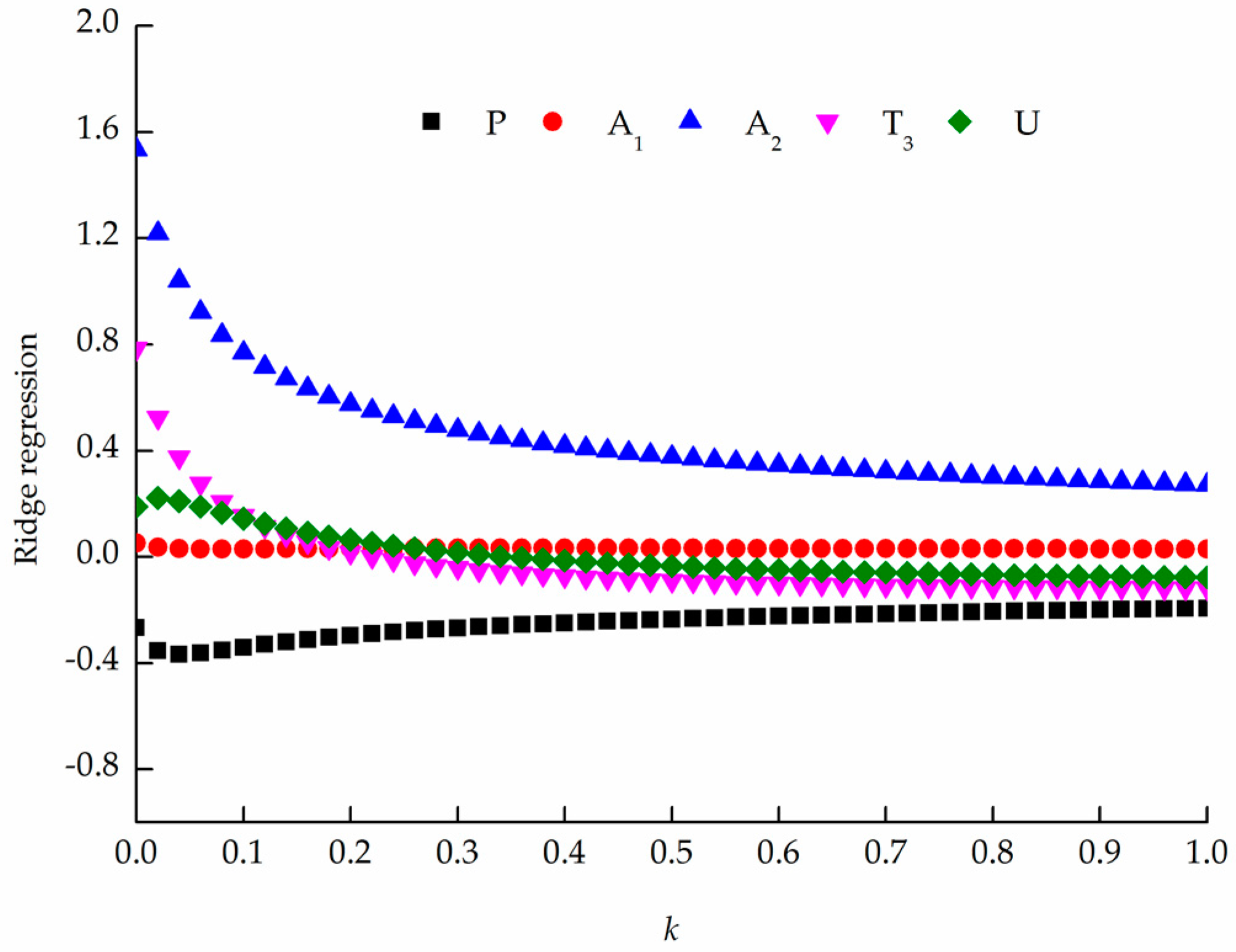
Based on the calculation of the agricultural WF within Beijing from 1980 to 2012, this paper analyzed the influence of anthropogenic factors on the water footprint using the STIRPAT model. From the results of the ridge regression estimation, we know that the model simulation results are significant. Based on their coefficients, population, urbanization, GDP, the Engel coefficient, and total rural power all have different influences on the agricultural WF within Beijing.
In the middle of 1970s, the United Nations Food and Agriculture Organization (FAO) adopted the Engel coefficient as one of the important criteria to evaluate the living standards in a country or region. The Engel coefficient of Beijing has decreased from 55.3% in 1980 to 31.3% in 2012. According to the life criterion of the FAO, during the past three decades, the living standard of Beijing citizens has changed from “adequate food and clothing” to “richness” and is approaching “the most rich.” The Engel coefficient has the largest influence and the most positive driving force for the increase in the WF. With China's reform and opening up in 1978, social productive forces rapidly developed. In Beijing, as the capital of China, the people’s living standard has greatly changed. Residents are no longer satisfied with the provision of enough food and clothing but also tend to pursue a quality lifestyle characterized by a balanced diet structure, nutritious food, and even luxury products [43]. According to the principle of the Environmental Kuznets Curve (EKC) [44], there is an inverted U-shaped relationship between environmental pressure and economic growth [28]. In this paper, the relationship between the Engel coefficient and the agricultural WF within Beijing has no environmental Kuznets curve during the study period, which is similar to China. This means that economic development and water conservation have not yet achieved synergy. Urbanization also increases the WF. The urbanization of Beijing has risen from 57.629% in 1980 to 86.198% in 2012 [33]. Due to its steady growth during the past 30 years, urbanization still plays a significant role in the agricultural WF within Beijing.
Population, as the largest inhibited factor of the agricultural WF within Beijing, has risen from 9.043 million to 20.693 million from 1980 to 2012. This is in contrast to the situation in China. For the whole country, population is a positive driving force for increases in the agricultural WF [22]. The rapid population growth in China has led to increased demand for crops, which has directly led to an increase in the WF. However, for Beijing, the political center of China, the sown area of crops has decreased with the increase in population. The sown area of crops has strongly decreased from 6570 km2 to 2830 km2 [33]. This causes a reduction in the agricultural WF within Beijing.
Total rural power, as a measure of technical development, is a very important index that reflects the development of agricultural mechanization in an area. Total rural power plays an inhibitory role in the agricultural WF within Beijing. From 1980 to 2012, total rural power has grown more than sixfold. Similar to the results of other studies, other scholars found that, in China, technology has contributed to a decline in energy intensity [
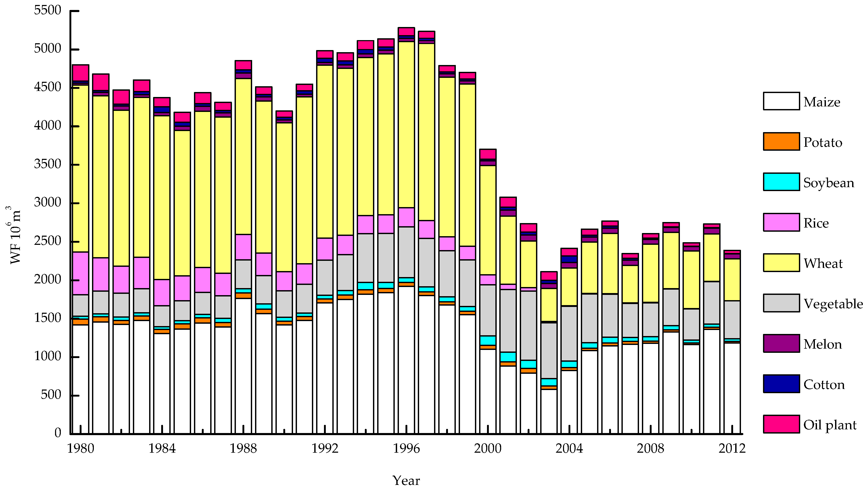
45]. On the one hand, planting technology in Beijing has significantly improved. With the development of water-saving irrigation technology, Beijing has used sprinkler irrigation, micro irrigation, mechanical film, and mechanized furrow sowing instead of the traditional irrigation. For instance, the Tongzhou district applied the integrated management of water and fertilizer in 2005, which significantly improved the water use efficiency under protected cultivation. In addition, Beijing has actively promoted the mechanization of agriculture. In 1980, Beijing only had 2755 motorized sprayers, but there were 29,505 units in 2012. These technologies have effectively solved the problems of agricultural water shortage, poor water storage capacity, and the low efficiency of irrigation water, which have a significant impact on the reduction in the use of agricultural water within Beijing [46]. On the other hand, Beijing has an adjusted plantation structure. Rain-fed maize has largely replaced wheat planting in Beijing, which is also reflected in Figure 1, which will drastically reduce the blue WF.
GDP also has an inhibitory influence on the agricultural WF with Beijing during the study period, with an elastic coefficient of −0.078. The per capita GDP in Beijing has increased from $1,009 to $13,857, a 13-fold increase [33]. Since China joined the WTO in 2001, Beijing has actively adjusted the direction of development and made an effort to establish a resource-saving industrial structure and an export-oriented trade structure; as a result, Beijing has imported large quantities of agricultural products from other regions [47]. Trade in agricultural products not only plays a positive role in ensuring the healthy development of the social economy of Beijing but also inhibits the agricultural WF within Beijing.

5. Conclusions and Policy Implications

The quantitative analysis of the impact of anthropogenic factors on the water footprint is a hot spot in terms of research on water sustainability. In this paper, the extended STIRPAT model and the ridge regression method are employed to examine the factors that influence the agricultural WF within Beijing from 1980 to 2012.
The utilization of water resources in Beijing is unsustainable, and the prominent contradiction between supply and demand has become a social and economic development bottleneck [48]. In this paper, we calculated the agricultural WF within Beijing from the production point of view. The optimization and adjustment of agricultural planting structures and the improvement of agricultural water saving technology are the keys to relieving the shortage of water resources in Beijing.
First, Beijing should increase the use of water-saving technology to decrease the agricultural WF. From Equation (16), we know that technology reduces the use of water in agriculture in Beijing. Water-saving technology can use limited water resources in the most effective way. Compared with flood irrigation, water-saving well irrigation, deep plowing, soil moisture maintenance, the selection of drought-resistant varieties, and other agronomic water-saving techniques should be widely promoted. In addition, the government can build a number of modern and efficient agricultural parks and modern agricultural enterprises in order to promote the industrialization of high-tech agriculture.
Second, water regulation and environmental management in Beijing should place greater emphasis on the plantation structure. Beijing is seriously lacking in water. In addition to considering market-oriented changes, Beijing must also give full consideration to the limits of local resources and the carrying capacity, especially the water supply capacity, when adjusting to the plantation structure. According to the calculation of the agricultural WF, the WF of wheat and rice are very large. Therefore, the crops with small WF, such as maize, vegetables, and melons, should be given priority for cultivation, and the planting of wheat and rice should be discouraged. Beijing can import crops with large WF from water-rich regions to ease the pressure of water resources, which will be cheaper than water transfer projects [49].

Acknowledgments

This study was supported by National Natural Science Foundation of China (41301636, 51474033) and the Beijing Natural Science Foundation (9122017).

Author Contributions

Kai Huang conceived and designed the study; Chen Jin analyzed the data; Chen Jin wrote the paper; Yajuan Yu, Yue Zhang, and Kai Huang helped to revise the manuscript.

Conflicts of Interest

The authors declare no conflict of interest.

Appendix A

Table A1. Statistics of climatic factors used in CropWat software.
VariableMinMaxMeanSDCV
Precipitation (0.1 mm)0.0003276.60053.070172.8643.257
Wind Velocity (0.1 m/s)112.320345.600201.83340.1800.199
Min Temp (0.1 °C)−17.00021.2002.21111.0344.992
Max Temp (0.1 °C)3.30041.90025.06110.1090.403
Humidity (%)22.00083.00054.06112.9140.239
Sunshine Duration (h)3.57010.6407.0061.3300.190
Figure A1. Ridge trace curve.
Water 08 00513 g003

References

  1. Huang, K.; Wang, Z.; Yu, Y.; Yang, S. Assessing the environmental impact of the water footprint in Beijing, China. Water Policy 2015, 17, 557–560. [Google Scholar] [CrossRef]
  2. Beijing Bureau of Statistics (BBS). Beijing Statistics Yearbook; China Statistics Press: Beijing, China, 2015. (In Chinese)
  3. Beijing Water Authority (BWA). Beijing Water Resources Bulletin 2014; China Water and Hydropower Publisher: Beijing, China, 2015. (In Chinese)
  4. Sivakumar, B. Water crisis: From conflict to cooperation—An overview. Hydrol. Sci. J. 2011, 56, 531–552. [Google Scholar] [CrossRef]
  5. Siche, R.; Pereira, L.; Agostinho, F.; Ortega, E. Convergence of ecological footprint and emergy analysis as a sustainability indicator of countries: Peru as case study. Commun. Nonlinear Sci. 2010, 15, 3182–3192. [Google Scholar] [CrossRef]
  6. Senbel, M.; McDaniels, T.; Dowlatabadi, H. The Ecological Footprint: A non-monetary metric of human consumption applied to North America. Glob. Environ. Chang. 2003, 13, 83–100. [Google Scholar] [CrossRef]
  7. Hoekstra, A.Y.; Hung, P.Q. Virtual Water Trade: A Quantification of Virtual Water Flows between Nations in Relation to International Crop Trade; Value of Water Research Report Series No. 11; UNESCO-IHE: Delft, The Netherlands, 2002. [Google Scholar]
  8. Hoekstra, A.Y.; Chapagain, A.K.; Aldaya, M.M.; Mekonnen, M.M. Water Footprint Assessment Manual: Setting the Global Standard; Earthscan: London, UK, 2011. [Google Scholar]
  9. Manzardo, A.; Mazzi, A.; Loss, A.; Butler, M.; Williamson, A.; Scipioni, A. Lessons learned from the application of different water footprint approaches to compare different food packaging alternatives. J. Clean. Prod. 2016, 112, 4657–4666. [Google Scholar] [CrossRef]
  10. Hoekstra, A.Y. A critique on the water-scarcity weighted water footprint in LCA. Ecol. Indic. 2016, 66, 564–573. [Google Scholar] [CrossRef]
  11. Pfister, S.; Boulay, A.; Berger, M.; Hadjikakou, M.; Motoshita, M.; Hess, T.; Ridoutt, B.; Weinzettel, J.; Scherer, L.; Döll, P. Understanding the LCA and ISO water footprint: A response to Hoekstra “A critique on the water-scarcity weighted water footprint in LCA”. Ecol. Indic. 2017, 72, 352–359. [Google Scholar] [CrossRef]
  12. Pfister, S.; Ridoutt, B.G. Water Footprint: Pitfalls on Common Ground. Environ. Sci. Techol. 2014, 48, 4. [Google Scholar] [CrossRef] [PubMed]
  13. Hu, T.; Huang, K.; Yu, Y.; Zhang, X.; Xu, Y.; Wang, X. Measuring Water Footprint on a Lake Basin Scale: A Case Study of Lake Dianchi, China. Clean-Soil Air Water 2016, 44, 1296–1305. [Google Scholar] [CrossRef]
  14. Bulsink, F.; Hoekstra, A.Y.; Booij, M.J. The water footprint of Indonesian provinces related to the consumption of crop products. Hydrol. Earth Syst. Sci. 2010, 14, 119–128. [Google Scholar] [CrossRef]
  15. Ge, L.; Xie, G.; Zhang, C.; Li, S.; Qi, Y.; Cao, S.; He, T. An Evaluation of China’s Water Footprint. Water Resour. Manag. 2011, 25, 2633–2647. [Google Scholar] [CrossRef]
  16. Chen, Z.M.; Chen, G.Q. Virtual water accounting for the globalized world economy: National water footprint and international virtual water trade. Ecol. Indic. 2013, 28, 142–149. [Google Scholar] [CrossRef]
  17. Zhang, Z.; Yang, H.; Shi, M. Analyses of water footprint of Beijing in an interregional input–output framework. Ecol. Econ. 2011, 70, 2494–2502. [Google Scholar] [CrossRef]
  18. Wang, Z.; Huang, K.; Yang, S.; Yu, Y. An input–output approach to evaluate the water footprint and virtual water trade of Beijing, China. J. Clean. Prod. 2013, 42, 172–179. [Google Scholar] [CrossRef]
  19. Shiklomanov, I.A.; Rodda, J.C. World Water Resources at the Beginning of the Twenty-First Century; Cambridge University Press: Cambridge, UK, 2003; pp. 33–36. [Google Scholar]
  20. The Ministry of Water Resources of the People’s Republic of China. Chinese Water Resources Bulletin 2012; China Water and Hydropower Publisher: Beijing, China, 2012. (In Chinese)
  21. Wang, X.; Huang, K.; Yu, Y.; Hu, T.; Xu, Y. An input–output structural decomposition analysis of changes in sectoral water footprint in China. Ecol. Indic. 2016, 69, 26–34. [Google Scholar] [CrossRef]
  22. Zhao, C.; Chen, B. Driving force analysis of the agricultural water footprint in China based on the LMDI method. Environ. Sci. Technol. 2014, 48, 12723–12731. [Google Scholar] [CrossRef] [PubMed]
  23. Xu, Y.; Huang, K.; Yu, Y.; Wang, X. Changes in water footprint of crop production in Beijing from 1978 to 2012: A logarithmic mean Divisia index decomposition analysis. J. Clean. Prod. 2014, 87, 180–187. [Google Scholar] [CrossRef]
  24. Zhao, C.; Chen, B.; Hayat, T.; Alsaedi, A.; Ahmad, B. Driving force analysis of water footprint change based on extended STIRPAT model: Evidence from the Chinese agricultural sector. Ecol. Indic. 2014, 47, 43–49. [Google Scholar] [CrossRef]
  25. Dietz, T.; Rosa, E.A. Effects of Population and Affluence on CO2 Emissions. Proc. Natl. Acad. Sci. USA 1997, 94, 175–179. [Google Scholar] [CrossRef] [PubMed]
  26. Dietz, T.; Rosa, E.A. Rethinking the environmental impacts of population, affluence and technology. Hum. Ecol. Rev. 1994, 1, 277–300. [Google Scholar]
  27. York, R.; Rosa, E.A.; Dietz, T. STIRPAT, IPAT and ImPACT: Analytic tools for unpacking the driving forces of environmental impacts. Ecol. Econ. 2003, 46, 351–365. [Google Scholar] [CrossRef]
  28. Wang, P.; Wu, W.; Zhu, B.; Wei, Y. Examining the impact factors of energy-related CO2 emissions using the STIRPAT model in Guangdong Province, China. Appl. Energy 2013, 106, 65–71. [Google Scholar] [CrossRef]
  29. Jia, J.; Deng, H.; Duan, J.; Zhao, J. Analysis of the major drivers of the ecological footprint using the STIRPAT model and the PLS method—A case study in Henan Province, China. Ecol. Econ. 2009, 68, 2818–2824. [Google Scholar] [CrossRef]
  30. Liddle, B. Age-structure, urbanization, and climate change in developed countries: Revisiting STIRPAT for disaggregated population and consumption-related environmental impacts. Popul. Environ. 2010, 31, 317–343. [Google Scholar] [CrossRef]
  31. Martínez-Zarzoso, I.; Maruotti, A. The impact of urbanization on CO2 emissions: Evidence from developing countries. Ecol. Econ. 2011, 70, 1344–1353. [Google Scholar] [CrossRef]
  32. Madu, I.A. The impacts of anthropogenic factors on the environment in Nigeria. J. Environ. Manag. 2009, 90, 1422–1426. [Google Scholar] [CrossRef] [PubMed]
  33. Beijing Bureau of Statistics (BBS). Beijing Statistics Yearbook; China Statistics Press: Beijing, China, 1980–2013. (In Chinese)
  34. Chapagain, A.K.; Hoekstra, A.Y.; Savenije, H.H.G.; Gautam, R. The water footprint of cotton consumption: An assessment of the impact of worldwide consumption of cotton products on the water resources in the cotton producing countries. Ecol. Econ. 2006, 60, 186–203. [Google Scholar] [CrossRef]
  35. Food and Agriculture Organization of the United Nations (FAO). Cropwat Model; FAO: Rome, Italy, 2003. [Google Scholar]
  36. Allen, R.G.; Pereira, L.S.; Raes, D.; Smith, M. Evapotranspiration Guidelines for Computing Crop Water Requirements; Food and Agriculture Organization: Rome, Italy, 1998. [Google Scholar]
  37. Ehrlich, P.R.; Holdren, J.P. Impact of population growth. Science 1971, 171, 1212–1217. [Google Scholar] [CrossRef] [PubMed]
  38. Waggoner, P.E.; Ausubel, J.H. A framework for sustainability science: A renovated IPAT identity. Proc. Natl. Acad. Sci. USA 2002, 99, 7860–7865. [Google Scholar] [CrossRef] [PubMed]
  39. Hoerl, A.E.; Kennard, R.W. Ridge regression: Biased estimation for nonorthogonal problems. Technometrics 2000, 42, 80–86. [Google Scholar] [CrossRef]
  40. Farrar, D.E.; Glauber, R.R. Multicollinearity in regression analysis; the problem revisited. Rev. Econ. Stat. 1964, 49, 92–107. [Google Scholar] [CrossRef]
  41. China Meteorological Administration (CMA). China Meterological Data Sharing Service System; CMA: Beijing, China, 2014. Available online: http://cdc.cma.gov.cn/ (accessed on 19 February 2015).
  42. Chen, Y.; Tian, P. Application of ridge regression in the capital structure influencing factor regression modeling. Stat. Decis. 2006, 5, 125–126. (In Chinese) [Google Scholar]
  43. Hubacek, K.; Guan, D.; Barrett, J.; Wiedmann, T. Environmental implications of urbanization and lifestyle change in China: Ecological and Water Footprints. J. Clean. Prod. 2009, 17, 1241–1248. [Google Scholar] [CrossRef]
  44. Lin, B.Q.; Jiang, Z.J. Kuznets curve prediction and influence factors of China’s CO2 emission. Manag. World 2009, 4, 27–36. (In Chinese) [Google Scholar]
  45. Xia, Y. The impact of technology and structure change on GHG emissions in China: An analysis based on LMDI model. Int. J. Glob. Warm 2011, 3, 307–327. [Google Scholar] [CrossRef]
  46. Deng, X.P.; Shan, L.; Zhang, H.; Turner, N.C. Improving agricultural water use efficiency in arid and semiarid areas of China. Agric. Water Manag. 2006, 80, 23–40. [Google Scholar] [CrossRef]
  47. Huang, J.; Zhang, H.L.; Tong, W.J.; Chen, F. The impact of local crops consumption on the water resources in Beijing. J. Clean. Prod. 2012, 21, 45–50. [Google Scholar] [CrossRef]
  48. Huang, J.; Song, Z.; Fu, C. Characteristics of water footprint and agricultural water structure in Beijing. Acta Ecol. Sin. 2010, 30, 6546–6554. (In Chinese) [Google Scholar]
  49. Bouwer, H. Integrated water management: Emerging issues and challenges. Agric. Water Manag. 2000, 45, 217–228. [Google Scholar] [CrossRef]
Figure 1. Changes in the agricultural water footprint within Beijing from 1980 to 2012.
Water 08 00513 g001
Figure 2. Changes in the blue, green, and grey water footprint of crop production within Beijing from 1980 to 2012.
Water 08 00513 g002
Table 1. Variables in the extended STIRPAT model.
Independent VariablesDefinition of Measuring MethodUnit of Measurement
P—population million
U—urbanization levelthe percent of urban population on the total population%
A1—economic levelGDP per capitaUS dollar
A2—living standardEngel coefficient%
T1—Cultivated land levelland demand per crop yieldHectare/10 thousand tons
T2—technical levelvolume of chemical fertilizer use1 × 104 ton
T3—technical leveltotal rural power consumption1 × 104 kwh
Table 2. Univariate statistical analysis of the alternative driving factors.
VariableMinMaxMeanSDCV
P (million)904.3002069.3001310.745339.0010.259
A1 (US dollar)115.9001217.000503.00161.3010.122
A2 (%)30.90054.10042.2011.4020.033
U (%)0.5760.8620.7340.1000.137
T1 (Hectare/10 thousand tons)0.1527.52932.2212.3301.049
T2 (1 × 10⁴ ton)8.20019.80014.2733.0910.217
T3 (1 × 10⁴ kwh)76,753619,806281,00627,601.7760.098
Notes: SD is the standard deviation; CV is the coefficient of variation.
Table 3. Matrix of correlations between variables.
PA1A2UT1T2T3
WFPearson correlations−0.800 **−0.833 **0.887 **−0.633 **−0.2490.141−0.754 **
Sig.0.0000.0000.0000.0000.1620.4330.000
Notes: Sig. means significance; ** means significance at the 1% level.
Table 4. Results of the unit root test.
Value IPA1A2UT3D(I)D(P)D(A1)D(A2)D(U)D(T3)
t-statistic −0.5221.7412.260−0.861−1.1532.260−5.076−4.862−4.657−5.095−5.582−5.076
Test critical values1% level−3.654−3.654−3.654−3.654−3.654−3.654−3.662−3.662−3.689−3.662−3.662−3.662
5% level−2.957−2.957−2.957−2.957−2.957−2.957−2.960−2.960−2.972−2.960−2.960−2.960
10% level−2.617−2.617−2.617−2.617−2.617−2.617−2.619−2.619−2.625−2.619−2.619−2.619
Notes: I represents the total water footprint; D(I) is the first difference sequences of I.
Table 5. Influencing factors of water footprint by ordinary least squares (OLS).
VariableUnstandardized CoefficientsStd. Errort-StatisticSig.VIF
C10.3162.3174.4520.000
lnP−0.3580.418−0.8580.39838.551
lnA10.0230.1080.2140.83237.843
lnA22.2580.3167.1430.00014.377
lnU0.4040.2871.4090.1706.147
lnT30.3210.0804.0200.0009.225
R-squared0.919Adjusted R squared0.904
F-statistic61.562Sig.0.000
Durbin–Watson1.896
Notes: Std. error is the standard error; Sig. means significance; VIF is the variance inflation factor.
Table 6. Ridge regression results (k = 0.5).
ItemsNon-Normalized CoefficientNormalized CoefficientVIFSig.
P−0.2010.0490.2480.00
A1−0.0780.0130.1790.00
A20.5790.0760.1320.00
T3−0.0210.1280.1320.045
U0.0960.0260.1270.044
Constant22.4970.8040.0370

