Article

Unified Analysis of Multi-Chamber Contact Tanks and Mixing Efficiency Based on Vorticity Field. Part I: Hydrodynamic Analysis

1
Department of Civil Engineering, Eskisehir Osmangazi University, Eskisehir 26000, Turkey
2
Multimedia Environmental Simulations Laboratory, School of Civil and Environmental Engineering Georgia Institute of Technology, Atlanta, GA 30332, USA
*
Author to whom correspondence should be addressed.
Water 2016, 8(11), 495; https://doi.org/10.3390/w8110495
Submission received: 15 August 2016 / Revised: 9 October 2016 / Accepted: 24 October 2016 / Published: 2 November 2016
(This article belongs to the Special Issue Water Quality and Health)

Abstract

:
Multi-chamber contact tanks have been extensively used in industry for water treatment to provide potable water to communities, which is essential for human health. To evaluate the efficiency of this treatment process, flow and tracer transport analysis have been used in the literature using Reynolds averaged Navier–Stokes (RANS) and large-eddy simulations (LES). The purpose of this study is two-fold. First a unifying analysis of the flow field is presented and similarities and differences in the numerical results that were reported in the literature are discussed. Second, the vorticity field is identified as the key parameter to use in separating the mean flow (jet zone) and the recirculating zones. Based on the concepts of vorticity gradient and flexion product, it is demonstrated that the separation of the recirculation zone and the jet zone, fluid-fluid flow separation, is possible. The separation of the recirculation zones and vortex core lines are characterized using the definition of the Lamb vector. The separated regions are used to characterize the mixing efficiency in the chambers of the contact tank. This analysis indicates that the recirculation zone and jet zone formation are three-dimensional and require simulations over a long period of time to reach stability. It is recognized that the characteristics of the jet zones and the recirculation zones are distinct for each chamber and they follow a particular pattern and symmetry between the alternating chambers. Hydraulic efficiency coefficients calculated for each chamber show that the chambers having an inlet adjacent to the free surface may be designed to have larger volumes than the chambers having wall bounded inlets to improve the efficiency of the contact tank. This is a simple design alternative that would increase the efficiency of the system. Other observations made through the chamber analysis are also informative in redefining the characteristics of the efficiency of the contact tank system.

1. Introduction

In recent years multi-chamber contact tanks have gained wide applications in water treatment facilities using either chlorine or ozone treatment. An efficient contact tank mixing system is required for the ozonation process since ozone cannot dissolve in water as readily as chlorine. Energy requirements of the mixing process and the amount of ozone required during the process are proportional to the efficiency of mixing in the contact tank. Short-circuiting of mixing due to the development of recirculating flows and friction-induced energy losses are important problems that may reduce the performance of the contact tank.
Modifications of the contact tank design were proposed using horizontal baffles or turning vanes to increase the mixing efficiency of the contactor. In one study plug flow definitions were used to characterize the flow system [1]. Three-dimensional numerical simulations were conducted by Zachary et al. [2] in order to maximize the disinfection efficiency of the contactor by modifying the hydraulic design of baffles. Guiding walls were included in the contact tank in order to minimize the recirculation effects [3]. The relationship between the baffling performance and energy loss for the definition of “hydraulic efficiency” of the contact tank system was investigated by Zhang et al. [4], where the authors stated that the energy saving afforded by using more baffles in the contactor was offset by the extra energy necessary to drive the flow through the contact tank system.
In recent years, advances in computational power and numerical techniques have made it possible to simulate complex flows using computational fluid dynamics (CFD). Fluid flow in contact tank systems are one such flow system. Accurate computation of turbulent flow in the contact tank is required in order to evaluate the characteristics of the flow field of the contactor, which is necessary for efficiency analysis. In essence, the recirculating zones that develop in the chambers are responsible for reducing the efficiency of contact tanks and proper characterization of these zones is necessary to evaluate the efficiency of the contactor. A literature review on this subject indicates that CFD applications are necessary to simulate the dynamics of energetic eddies that are produced in spatial and time domains to accurately predict the formation of recirculation regions in each chamber.
In CFD modeling, three different approaches are used to simulate turbulent flows, Direct Numerical Simulation (DNS), Reynolds averaged Navier–Stokes (RANS), and large-eddy simulations (LES). The DNS approach requires extremely high computational resources and time since all of the turbulence scales are solved spatially and temporally without using a turbulence closure model. DNS of flow in a contact tank system has not been reported in the literature due to the high computational power and time required. RANS simulations were implemented successfully by several researchers [2,5,6,7,8,9,10] during the last decade. The steady state solutions of flow in the contactor can be obtained at relatively low computational cost with RANS. LES can be interpreted as a numerical approach between the DNS and RANS approaches since eddies are spatially filtered into large scales that are calculated directly and unresolved small components are modeled using an appropriate sub-grid scale (SGS) model. A typical LES analysis of flow in a contactor was reported by Kim et al. [10], in which they used a Smagorinsky SGS LES model. In their study they showed that the LES approach was more reliable in predicting the characteristic residence time than the RANS simulation. LES could accurately predict the smaller scale but energetically important eddies near the entrance of each chamber, while those eddies could not be captured by RANS simulations even though the same grid resolution was used in both cases since energetically important eddies can only be captured by LES [6]. The wake region of an ultraviolet disinfection study was largely underpredicted by the RANS simulation due to unsteady effects, whereas the LES approach yielded results consistent with the experimental observations [11]. Therefore, it is preferable to use the LES approach for accurate simulation of flow in contact tanks. This was also reported in the aforementioned studies.
Various flow zones occur in the flow field of a contact tank system such as recirculation regions and the jet region. Numerical and analytical constraints have been used in the literature to identify different flow zones having fluid/fluid or fluid/solid interfaces. A Lamb vector, defined as the cross-product of fluid velocity and vorticity ( L ω × u ), is used to characterize the high shear regions in swirling jets since the Lamb vector is zero in non-rotational flow zones [12,13]. The definition of the normalized helicity [14], which is the cosine of the angle between the velocity and vorticity vectors, was used to identify the separation and reattachment trajectory for a fluid–solid boundary. These studies highlighted that the definition of vorticity and dot or cross-product of vorticity with the velocity field could be employed to separate the complex flow fields having different properties such as recirculating and jet flow zones. In this study, in addition to these two definitions, we have introduced the definition of the gradient of the vorticity field to characterize these zones, which has performed effectively. To our knowledge, the vorticity gradient concept has not been used in the literature for flow zone separation in contact tanks. This approach proves to be an effective tool in the analysis of flow zone separation, which is essential for efficiency evaluation of the chambers of the contactor.
The main motivation of this study, aside from presenting a unified analysis of several numerical results reported in the literature, is to accurately characterize the effective mixing zones in the chambers of the contactor tank. Using this characterization, the purpose is to propose mixing efficiency indexes to evaluate the design of the contactors from a hydraulic point of view (Part I) and also from a chemical transport and mixing point of view (Part II) [15]. CFD simulations were conducted for the laboratory-scale contact tank using both RANS and LES simulations. The public domain OpenFoam [16] software was used in the numerical solution of the governing equations. Numerical results obtained were compared with the results reported in the literature to validate the current computational model and also to resolve the differences that are reported in the literature among several studies.
It is clear that the earlier studies that were conducted using similar mathematical models, boundary conditions, grids, and CFD models yielded numerical results that are surprisingly different from one another, as reported in the abovementioned literature. In this study we point to the possible differences in the analysis of numerical results that may have led to these differences. The vorticity field of the mean flow in the contactor was analyzed to characterize the recirculation zone and jet zone volumes in each chamber. This characterization was used in the definition of the hydraulic efficiency of the multi-chamber contactor in Part I of this paper. In Part II of this paper [15], this characterization will also be used in the efficiency definition for chemical transport analysis.

2. Mathematical Model

2.1. Governing Equations of Fluid Flow

Three-dimensional flow in the contact tank is governed by the following equations, which define mass conservation for incompressible flow and momentum conservation for turbulent flow, commonly identified as Navier–Stokes (NS) equations:
u i ¯ x i = 0
u i ¯ t + u i ¯ u j ¯ x j = 1 ρ p ¯ x j + 1 ρ ( τ i j ¯ + T i j ¯ ) x j + g i + f i ¯ ,
where u i and p are the velocity components in the i-direction (x, y, and z direction) and the pressure, respectively; t is the time, ρ is the fluid density, and xi and xj represent the Cartesian coordinates. The overbar indicates the time-averaged component for RANS and the resolved turbulence scales for LES. The term τ i j ¯ represents viscous stress, which describes the momentum transport due to molecular motion, given as
τ i j ¯ = 2 μ S i j ¯ ; S i j ¯ = ( u i ¯ / x j + u j ¯ / x i ) / 2 ,
where μ is the fluid viscosity and S i j ¯ is the strain rate tensor. Here T i j ¯ denotes the stress tensor T i j ¯ = ρ u i u j ¯ . In the RANS approach, the stress tensor is approximated employing Boussinesq’s approximation, in which the Reynolds stresses are modeled as the product of the strain rate tensor and turbulent viscosity:
ρ u i u j ¯ = μ t S ¯ i j 2 3 ρ k δ i j .
In Equation (4), μ t is the turbulent viscosity, k = u i u i ¯ / 2 is the turbulent kinetic energy, and δ ij is Kronecker delta. In this study, the k-ε turbulence closure model is used in RANS and the turbulent viscosity is approximated as
μ t = C μ k 2 ε ,
in which C μ = 0.09 and ε is the turbulent kinetic energy dissipation rate, which can be calculated as
ε = C μ 3 / 4 k 3 / 2 l 0 ,
where l 0 is the turbulent scale, calculated as
l 0 = κ y ,
where κ = 0.41 and y is the distance from the wall to the first grid point.
In the LES approach, turbulent eddies are filtered into large and small sizes based on the local grid sizes using the SGS model. The well-known SGS model developed by Smagorinsky [17] is based on the Boussinesq hypothesis and the SGS stresses are computed from the following equation:
T i j ¯ 1 3 τ k k S G S δ i j = 2 ν S G S S i j ¯ ,
where ν S G S is SGS eddy viscosity, which can be approximated from Equation (9). The isotropic part of the SGS stresses, T k k ¯ is added to the filtered pressure term:
ν t = ( C s Δ ) 2 | S i j ¯ | ; | S i j ¯ | = ( 2 S i j ¯ S i j ¯ ) 1 / 2 ,
in which Δ is filter size Δ = ( Δ x Δ y Δ z ) 1 / 3 and C s is the Smagorinsky constant. Implementation of the Smagorinsky SGS model has some drawbacks, since C s is flow-dependent and varies significantly near a wall in wall-bounded flows. In the classical Smagorinsky approach, the dissipative and backscattering effects due to energy transfer from the small to large scales (reversed energy flow) are not considered. In this study we performed numerical simulations using the Dynamic Smagorinsky SGS Model, in which this coefficient is locally and dynamically determined [18,19] using information contained in the resolved flow field during the simulation, which includes backscattering effects from small scale to large scale [19]. Inaccurate prediction of sub-grid scale dissipation caused by inaccurate development of the perturbations in transitional flows has been reported, even though absolutely dissipative sub-grid scale models such as the Smagorinsky model have been successful in fully turbulent flows [20].
A source term f i ¯ is added to the right-hand side of Equation (2) to drive the flow through the periodic boundary conditions, as shown in Figure 1. In the application of the periodic boundary conditions, an appropriate pressure gradient is adjusted in the flow domain to specify the bulk velocity at the inlet and outlet such that the volumetric flow rate tends to a desired value [16]. The source term is applied to all computational cells inside the flow domain without applying boundary conditions at the inlet and outlet since prescribing inlet boundary conditions for the turbulence is generally cumbersome for CFD applications.

2.2. Simulation Setup and Boundary Conditions

A three-dimensional view of the computational domain and the dimensions of the contact tank are shown schematically in Figure 1. The flow domain, chamber dimensions, and number of chambers are selected to be the same as the flow configuration studied in [6,10,21,22], in order to compare the numerical results obtained in this study with the results reported earlier. As seen in this figure, water enters the inlet of the tank on the left with constant discharge Q and emerges from the tank at the outlet on the right to maintain an approximately constant water level of H inside the tank. Experimental studies were also conducted in [23] for the same flow configuration in a tank with 12 chambers. In the present study, numerical simulations were performed on the truncated version of the physical domain, applying periodic boundary conditions at the inlet and outlet to reduce the computational time and exclude the turbulence intensity effects at the inlet, which are generally cumbersome to prescribe for the simulation of turbulent flows.
Numerical simulations were performed for Reynolds number Re = 2740, which is based on the hydraulic diameter ( h R = 4 A c / π , where A c is the area of the cross section at the inlet) and the bulk velocity ( U b u l k ) at the inlet. The Reynolds number of the flow corresponds to the same flow configuration in the previously reported experimental [23] and numerical studies [6,10].
A structured mesh system is employed in both RANS and LES simulations with grid clustering near the boundaries of the physical domain in order to capture the evolution of the flow characteristics due to the presence of large gradients in the vicinity of the walls. The number of computational cells in the domain and the dimensionless wall distance ( y + = y u τ / ν ) near the solid boundaries are important characteristics of the mesh system that need to be investigated rigorously in order to obtain mesh-independent numerical results. Various mesh configurations consisting of different numbers of computational cells and dimensionless wall distance were tested while comparing the numerical results. In this paper only the mesh-independent numerical results are reported for simplicity. The number of computational cells used in each direction (nx, ny, and nz) and the maximum value of dimensionless wall distance for the present grid resolution are given in Table 1, along with the mesh characteristics reported in [6,10]. In this study, a large number of mesh cells (about 1.7 million computational cells) are used in the numerical simulations to capture the dynamically varying eddies and energy cascade in turbulence.
Numerical simulations are conducted using OpenFoam [16], in which the governing equations are solved using the finite volume method on structured and unstructured grids. The non-uniform structured mesh system was generated using the blockMesh utility available in the OpenFoam package. Second-order accurate upwind scheme (linearUpwind) is utilized for the convective terms and a second-order accurate central differencing method (Gauss linear) is used for the treatment of the diffusive terms. Thus, the overall accuracy of the numerical method is second-order in space. In the RANS simulations, a steady-state solution of the governing equations was obtained iteratively using the solver simpleFoam, which is based on the semi-implicit method for pressure-linked equation (SIMPLE) algorithm to couple velocity and pressure. Iterations were terminated when the maximum residual of the momentum equations and k-ε equations were less than 1 × 10⁻⁵. The overall convergence of the steady state solver is controlled by the maximum allowable continuity equation residual, which is selected as 1 × 10⁻¹⁹ throughout this study. Note that the convergence criteria for the steady state solution are selected to be the same as in [6]. In the LES, unsteady simulation of the problem was carried out using the solver pimpleFoam available in OpenFoam, which is a time-implicit solver for large-time step calculation of transient flows. A second-order accurate implicit scheme (backward) is used for temporal discretization of the governing equations. The maximum allowable time step size for the stability was adjusted according to the Courant–Friedrich–Levy (CFL) number, which was set to 0.5 in this study. The time step size was adjusted internally so that the maximum CFL = 0.5 was maintained during the simulation. This resulted in a time step in the order of about 0.001 s, even though the preferred implicit solver could perform a stable transient solution for the CFL = 5.
Computational cells at the inlet and outlet of the computational domain are assigned as periodic cells in the pre-processing step of the solution by using topoSet utility in order to use the periodic (cyclic) boundary conditions at the inlet and outlet. No-slip conditions are imposed for the velocity components at the stationary walls of the domain. Wall functions were employed for turbulent kinetic energy k, energy dissipation rate ε , and turbulent viscosity ν t in the numerical solution of the related equations [6], ensuring that the first grid point of the mesh from the wall is placed within the viscous sublayer ( y + 11.6 ) , as can be seen in Table 1. Note that wall functions available in OpenFoam are valid in the viscous sublayer. The effects of roughness on the walls are not considered in this study in order to compare the present numerical results with the previous results under the same conditions, as reported in the literature. A symmetry boundary condition is applied at the top of the computational domain using zero-shear condition since free-surface effects are negligible for the present problem [6,10]. The numerical computations are performed in parallel on two separate Linux workstations with 24 processors and 32 processors employing standard Message Passing Interface (MPI) within the OpenFoam based on the domain decomposition strategy.

3. Model Validation

Hydraulic Simulations

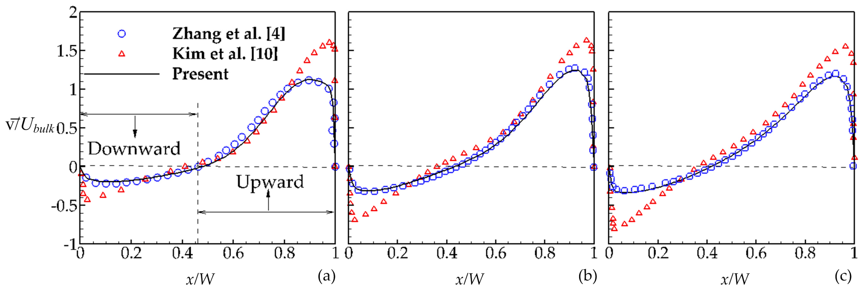
Span-wise averaged vertical velocity profiles obtained from RANS simulation are compared with the RANS results reported in the literature [4,10] at different vertical locations in the third chamber in Figure 2. The present numerical results are in good agreement with the results of [4]. However, some discrepancy is observed near the solid walls between the present results and [10]. The negative vertical velocity near the inlet of the chamber indicates that the flow in this region is in a downward direction, which indicates that the downward flow in this region is a part of the large circulating zone that develops in the third chamber to the left of the jet zone. This implies that in RANS solution there is one circulation zone and this outcome is different than the LES simulation results, which capture a second recirculation zone, as will be discussed later. The absence of a second recirculation region near the inlet of the third chamber shows that RANS simulation could not capture the dynamically important eddies, whereas in the LES results two counter-rotating recirculation regions have been observed in the vicinity of the inlet. In the RANS solution the flow direction changes from vertically negative to positive at x / W 0.46 along the chamber width, as shown in Figure 2a. This implies that a large recirculation region is occupying the region to the left of the jet region in the chamber. We note that the upward flow in the chamber occurs in both the recirculation and jet regions, which are separated by the separation layer. The key question that will be addressed in what follows is: How much of the upward flow is in the jet region and how much of it is in the recirculation region? This separation is important in defining the hydraulic efficiency of the chamber. Figure 2 also shows that the position of the peak velocity of the water jet shifts towards the wall horizontally as the flow develops in an upward direction.
The Reynolds number of the flow considered in this study is in transition range. The k-ε turbulence model selected in this application is more suitable for high Reynolds number flows, which may be used in the numerical simulation of full-scale contact tanks due to its lower computational power requirements in comparison to LES. The use of an improved low Reynolds number turbulence model would have been better, as was used in [9] to capture the hydrodynamics in water disinfection tanks for relatively low turbulence levels. In this study one purpose is the comparison of numerical results that were reported in the literature. Thus we have used the k-ε model to be consistent with those cases.
A series of LES runs were conducted in order to capture the dynamically varying large eddies in the tank and to achieve a validated time-averaged flow field. Flow parameters evaluated in the LES are in terms of mean flow and its turbulent fluctuating components since the flow field in the contact tank is characterized by time-varying turbulence effects. This is due to the action of the energetic coherent eddies, especially in the vicinity of the corner of the baffles at the inlet that creates the turbulent wakes to enter into the chamber. In the validation process of the LES results, some discrepancy has been observed between the previously reported LES results [6,10] and the results obtained in this study. This discrepancy was also evident in between these studies as well [6,10]. A comprehensive data analysis needs to be carried out to resolve this issue and to determine when the turbulent flow in the tank reaches mean flow spatially and temporally and over what period these time averages are to be computed for proper comparison of the results. Since the hydraulic efficiency analysis will be based on the time-averaged flow field in the later stages of this study, this characterization is important for that purpose as well.
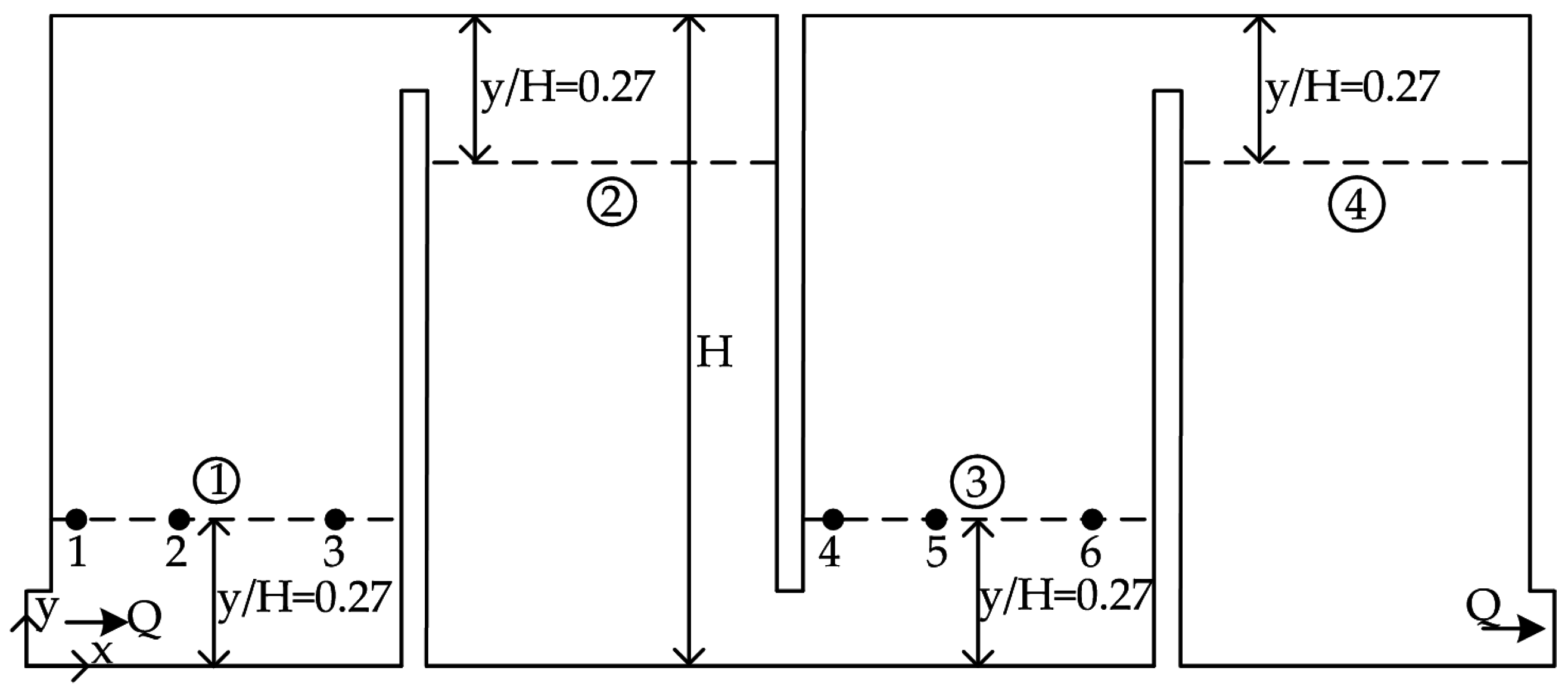
The LES run was performed for 400 s. To analyze the mean flow chamber-by-chamber, four sampling lines are placed within the contact tank at the same coordinates of the velocity profiles, as reported in [6,10]. The location of these lines can be seen in Figure 3 for each chamber. Mean velocity magnitudes and pressure are recorded for 100 points on each line and written to output files at t = 5 s time intervals during the simulation duration of 400 s. The Euclidean norm can be used to evaluate the variation of a mean quantity ϕ between two successive time levels, n − 1 and n. In this equation the subscript i refers to the points sampled on the line and ϕ may represent either the velocity or the pressure; m is the chamber number:
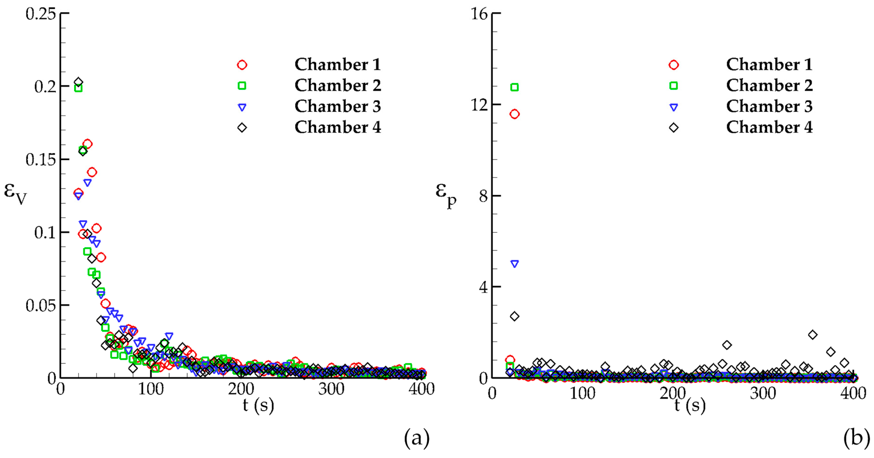
ε m ( n ) = [ i = 1 100 ( ϕ i n ϕ i n 1 ) 2 i = 1 100 ( ϕ i n 1 ) 2 ] 1 / 2 ; m = 1 , 2 , 3 , 4 .
The variation of ε m for velocity and pressure with time at each sampling line is shown in Figure 4. It can be seen in this figure that the difference between two successive time levels is high at the initial stages of the simulation and this difference starts to decrease as the flow reaches the mean flow condition as a function of time. This occurs after approximately t = 300 s, which corresponds to approximately 300,000 time steps since time step size is variable during a simulation based on the Courant stability condition. Note that the LES mean results in [10] were obtained using Δt = 0.005 s and at 10,000 time steps, which corresponds to t = 50 s. The output data is scattered in the early stages of the simulation at t = 50 s, which collapses to a narrow band as the simulation time increases. The results shown in Figure 4 indicate that the flow in the contact tank reaches almost mean flow spatially after t ≈ 300 s in this simulation. It would be useful to compare the duration to a characteristic time scale. Theoretical mean residence time can be used as a characteristic time scale for the contact tank system studied, which is defined as the ratio of the volume of the tank to the flow rate. The theoretical mean residence time is calculated as τ = 109.2 s for the present contact tank. Finally, a numerical simulation needs to be performed during about 3τ in order to obtain a time-averaged flow field.
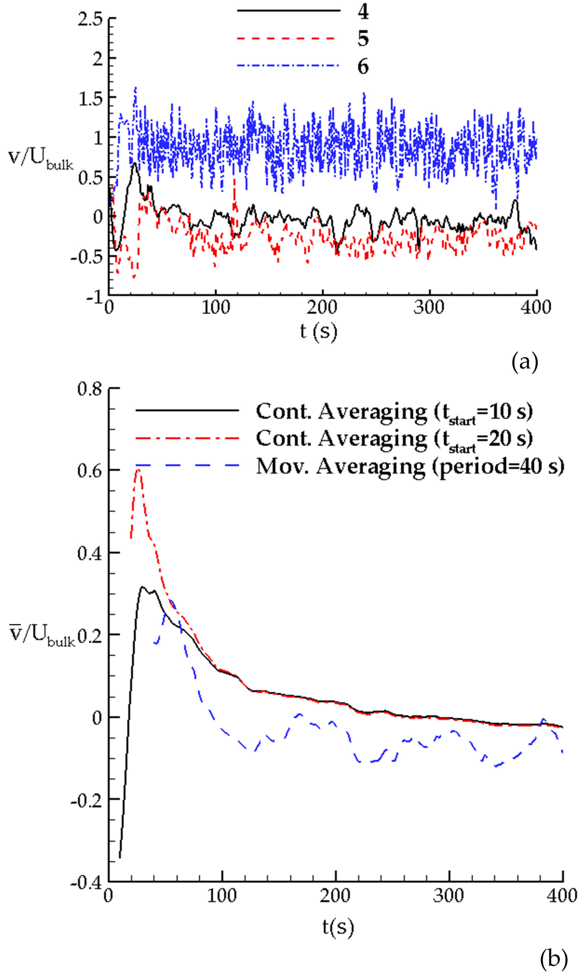
The time variations of instantaneous vertical velocities on the six points in Figure 4 are recorded at each time step of the simulation and plotted in Figure 5. These are normalized values using the bulk velocity at the inlet. Locations of the points were selected such that the large eddies would be dominant and peak values of the mean velocity profiles given in the literature could be captured (Figure 3). One can observe from this figure that the intensity of turbulence is higher in the jet region compared to those in the wake region due to the high velocity magnitudes and momentum in vertical direction in the jet. As can be seen from Figure 4a, it takes longer for the mean flow properties to establish in the wake region due to the time it takes for the wake effects to develop behind the baffle, whereas the flow reaches the mean flow values in a shorter period in the jet region. Thus the wake region requires more time to stabilize than the jet region, which should not be ignored when characterizing the mean flow conditions in the chamber. Thus, we can conclude that the stability characteristics of the wake region determine the time required to achieve mean flow conditions in the chambers and not the stability of the jet region. The direction of the vertical velocity at Point 4 is downward in the initial stages of the flow development since the momentum of recirculating flow in the large recirculation region that is separated from the jet flow forces the flow particles in the wake near the wall to move in the downward direction temporarily. Then, with the effect of dynamically important eddies near the entrance, the flow particles in the vicinity of the baffle move in the upward direction, which is evidence of formation of a counter-rotating second recirculation zone near the chamber inlet, with a maximum positive value at t ≈ 24 s. It takes about 300 s to develop a mean-flow in the wake region, as can be seen in Figure 4a and Figure 5a.
Different averaging procedures can be used to identify the possibility of oscillations in instantaneous velocity at Point 4. Similar oscillations are not observed in the jet region since this region stabilizes very fast. This is another reason why the mean flow conditions should be based not on the evaluation of the mean flow stabilization in the jet region but on the stabilization of the wake region. The stabilization of the recirculation zone and the determination of recirculation zone volumes will be described in the following sections. The time variations of calculated time-averaged values are plotted in Figure 5b in order to see the effect of different averaging procedures used to obtain mean flow field in the wake region. The time-averaged value of dimensionless vertical velocity at Point 4 was reported as 0.4 in [6]. The same time-averaged value can be obtained by using different averaging methods and periods, namely continuous and moving averaging, as can be seen in Figure 5b. This observation shows that when the continuous averaging is performed from t = 20 s to t = 41.4 s, the computed mean velocity is the same as the value that was obtained by using a moving average for 20 s at the same instant of time. Thus, in the present LES results, the capture of the same peak value as 0.4 is possible [6] if the same averaging period is used. However, this comparison cannot be validated since the time period used in the averaging process was not given in [6]. As can be seen in 
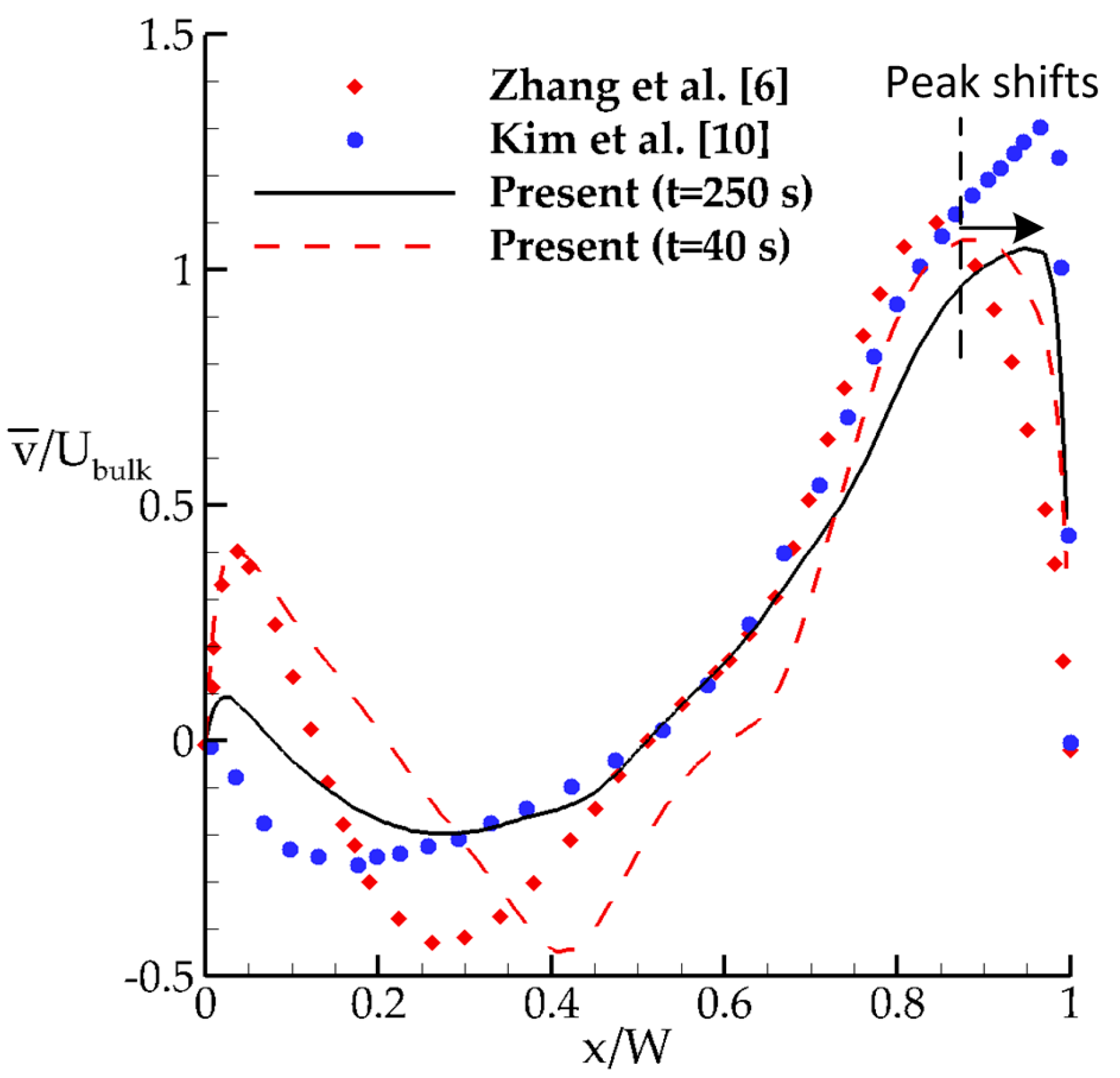
Figure 5b, this peak value decreases with time as the recirculation zone behind the baffle inlet develops. Thus, to show the effect of longer simulations on the averaging process, the time-averaged flow profile is compared with the results at previous instants of time and also with the previously reported numerical results [6,10] in Figure 6.
As can be seen in Figure 6, there is a significant difference between the previously published LES results that appeared in the literature. This may be due to the use of different averaging periods and the starting time of this averaging process. The magnitudes of the velocity profile obtained in this study at t = 40 s is consistent with the results of [6], showing that the LES gives a higher vertical velocity at the initial stages of the simulation. However, the peak value of the velocity profile starts to decrease as can be seen in Figure 5b and Figure 6. This detailed analysis of different time-averaging data for the same flow conditions may show that the LES results reported in [6] were probably obtained before the flow field in the chamber reaches the mean flow conditions with respect to wake parameters. It should be noted that the peak value of the jet flow is also shifting towards the wall with time as the flow develops, which is consistent with the results of [10]. This may explain some of the differences that are reported in the literature. Probably all results are correct for the time averaging periods that are used. We were not able to confirm this since the time averaging periods used were not reported in earlier studies. However, we conclude that a minimum of 300 s simulation time is necessary for the stabilization of the flow in the wake region and the mean flow analysis in the chamber should be based on this period. The pressure parameter is not a sensitive indicator of mean flow in the chamber (Figure 4b). Thus, pressure cannot be used to characterize the mean flow in the chamber.
It should be mentioned here that the effects of wall roughness are not considered in this study in order to be consistent with the previously reported numerical results. However, the effects of wall roughness must be considered at the implementation of wall functions in order to compare the numerical results with the experimental results, which are available for the hydrodynamics of contact tanks [9,24,25,26,27,28].
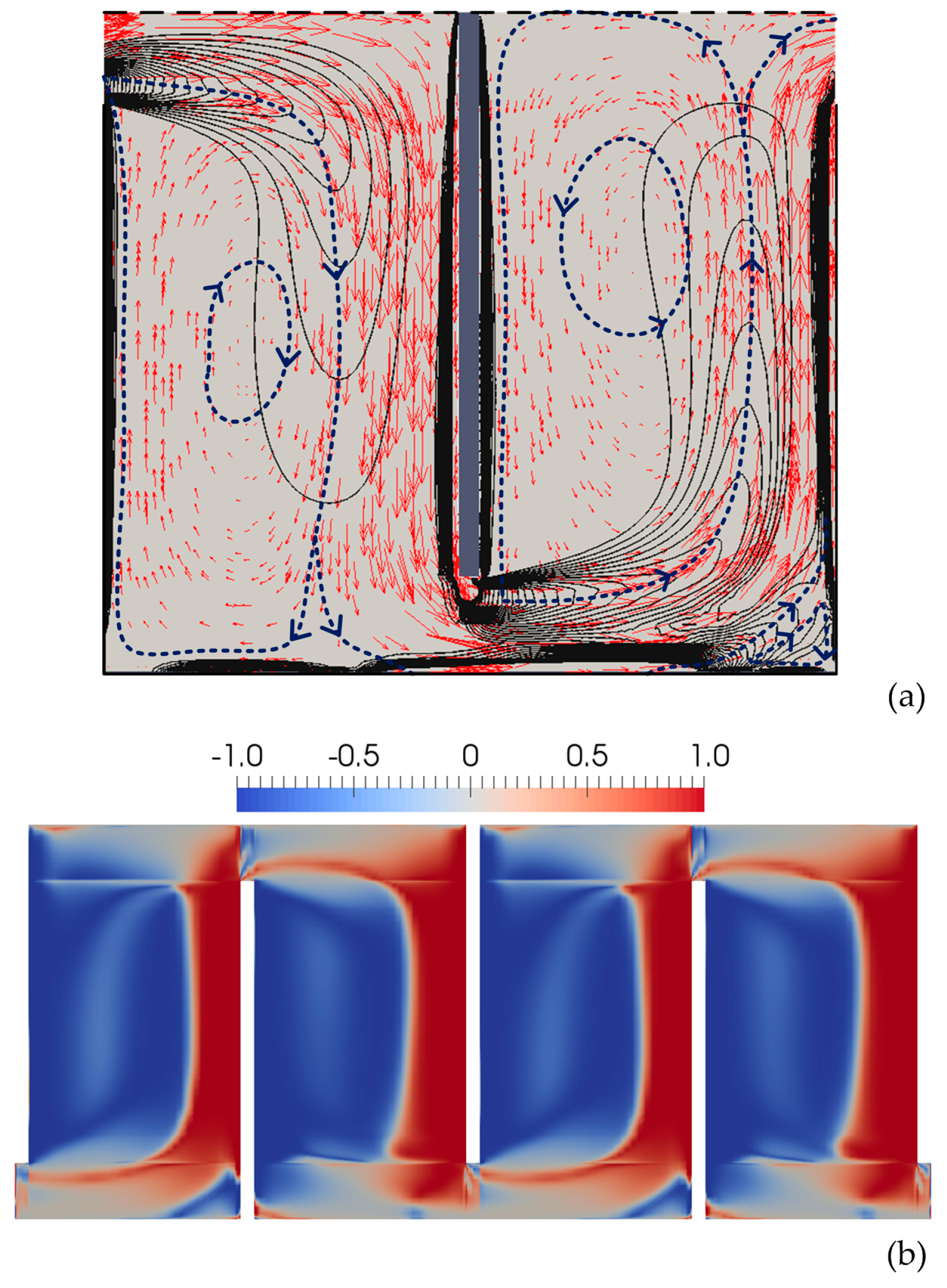
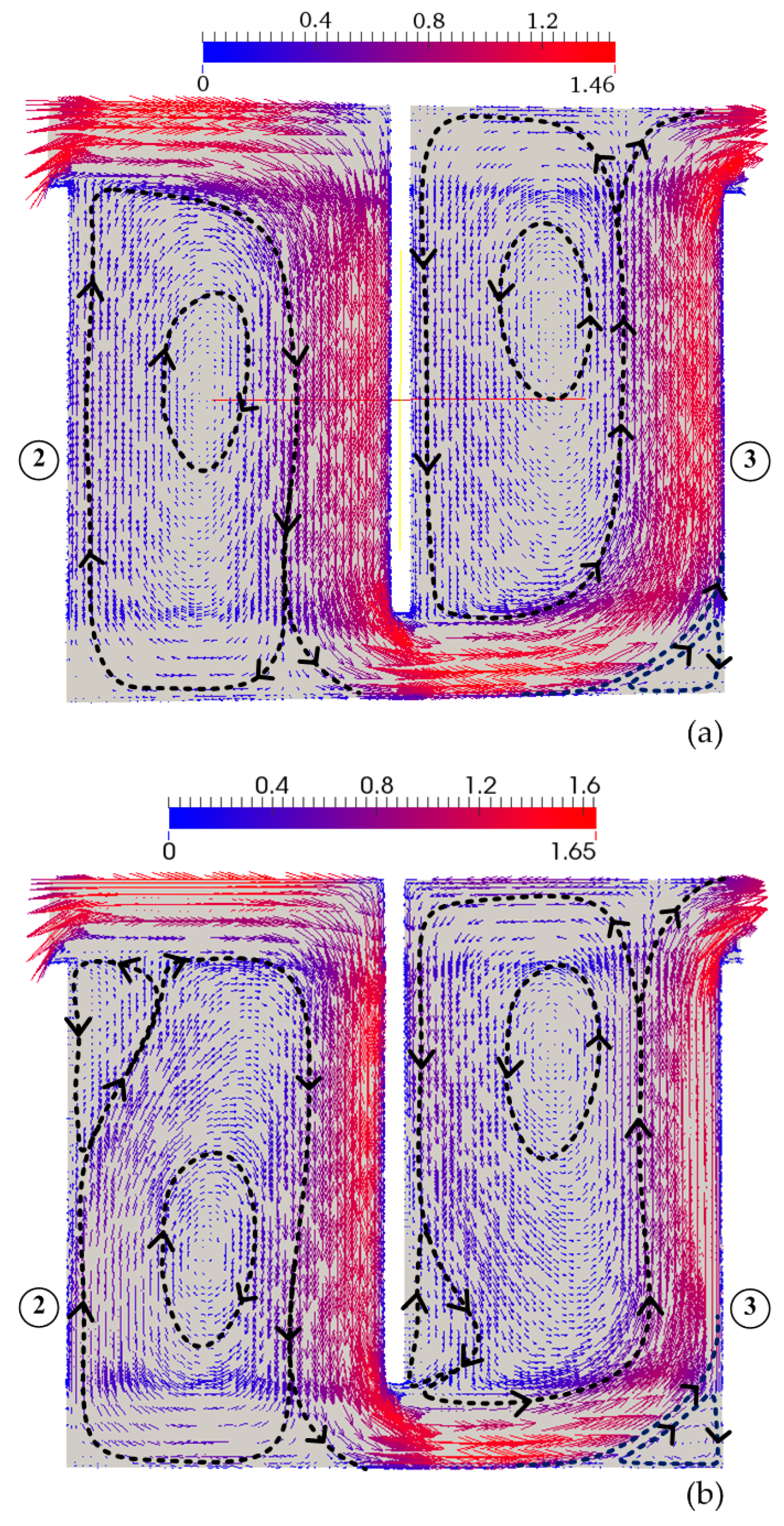
Velocity vectors along with the flow patterns represented by the dashed lines are shown for both steady state flow field in RANS and time-averaged flow field in LES in Figure 7. Steady state flow field in RANS (Figure 7a) depicts a large recirculation region and jet region in Chamber 2, whereas two recirculation zones and a jet region are encountered in Chamber 3, showing that the flow characteristics are not identical in adjacent chambers. Short-circuiting effects in Chamber 3 are greater than in Chamber 2 since the thickness of the jet region in Chamber 3 is smaller due to the presence of a short recirculation zone at the right-bottom corner of Chamber 3 and a relatively larger recirculation zone. Flow velocity in the jet region will increase as the thickness of the jet gets smaller to pass the same flow rate through a smaller fluid volume, which is responsible for the short-circuiting effects. The vertical location of the center of the recirculation region in Chamber 2 is below the center of recirculation zone in Chamber 3, which will be also shown later by the definition of the Lamb vector in order to locate the vortex core line accurately.
In LES results, another recirculation zone is encountered in the vicinity of the inlet of the chamber due to energetically important eddies near the sharp edge of the baffle, which could only be simulated in LES as shown in Figure 7b, even though the same grid resolution was used in RANS. This comparison of flow patterns in RANS and LES shows that RANS could not capture the unsteady entrance effects due to the energetic eddies since only time-averaged field of turbulence effects are simulated in RANS. The thickness of the flow jet reduces in LES due to the presence of the wake region at the entrance of the chamber, which produces a greater maximum dimensionless flow velocity of 1.65 in the jet flow, which is 13% higher than the maximum flow velocity obtained in RANS.
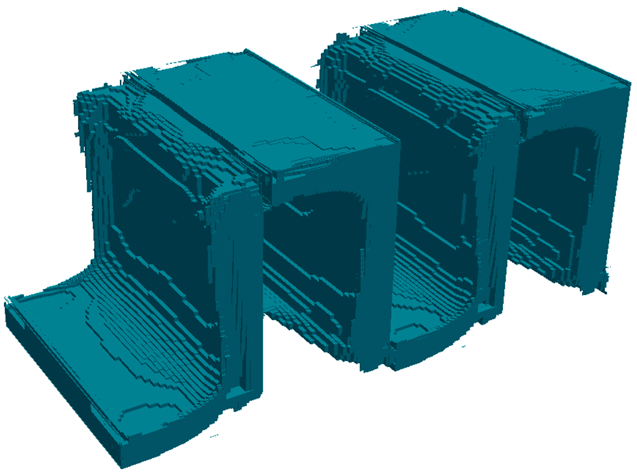
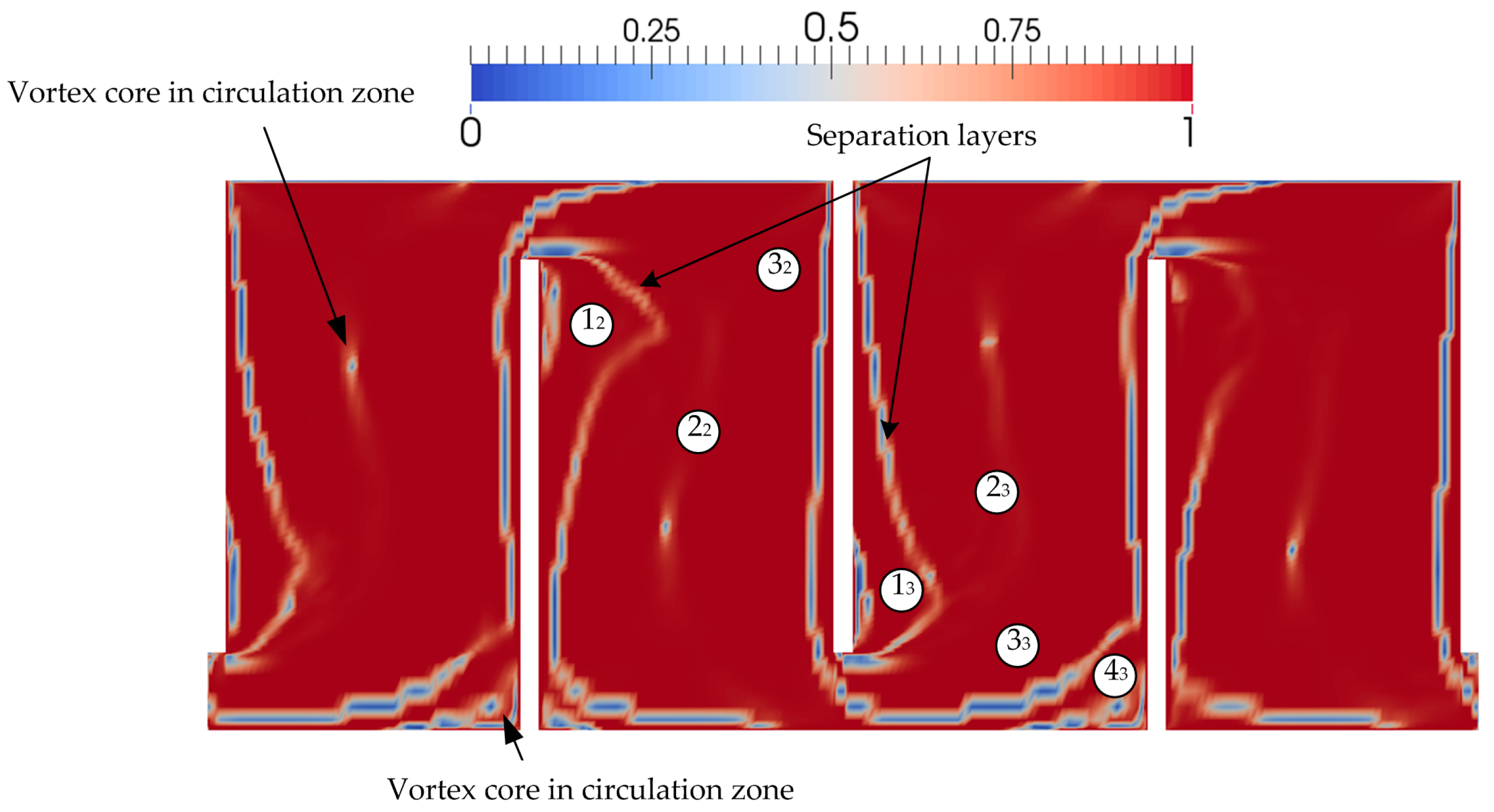
Based on the LES studies conducted in the present study, the general structure of the time-averaged flow field in the tank has been identified as shown in Figure 8 schematically. Large (22 and 23) and small (43) recirculating regions are evolving in the chambers, separated from each other by water jets (32 and 33). Here the capital number shows the zone number and the subscript shows the chamber number. The separation layer between the jet region and recirculation region develops at the inlet of the chamber and impinges on the right baffle at approximately the same elevation as the inlet, which can also be seen in Figure 7b. Similar behavior has been observed in the adjacent flow pattern between the jet region and recirculation region in Chamber 2, in which the flow tends to separate from the mean flow when it approaches the outlet opening. This observation shows that the baffle opening has a positive effect on the efficiency of the chamber at reducing the areas of the recirculation regions. The flow field in the downward and upward directions in Chambers 2 and 3 can theoretically be separated by a layer that splits the region into recirculation and jet flow regions. The separation layer could be identified based on the flow characteristics. Different definitions are available in the literature to distinguish rotational (recirculation zones) from the mean flow (jet region), as mentioned earlier.
In addition to primary recirculation regions, a secondary recirculation region has been observed at the upper and lower parts of the inlet of Chambers 2 and 3, respectively. It should be noted that the small recirculation regions (12 and 13) correspond to the energetically dynamic eddies in the vicinity of the sharp corner of the baffles, which could be captured by LES only. In this study, gradient of vorticity and flexion product concepts will be employed to identify the separation layer.
Three recirculation regions are encountered in Chamber 3, whereas only two recirculation zones appear in Chamber 2 since the free-slip boundary condition (less resistance) at the top of the computational domain does not allow the evolution of a recirculation zone at the upper right corner of Chamber 2. A recirculation zone cannot be observed at the bottom left corner of Chamber 2 due to low flow velocities near the corner. This observation confirms that the flow characteristics in each chamber are distinct, and thus the hydraulic efficiency of each chamber is not identical.

4. Vorticity Analysis for RANS and LES

The mean vorticity vector field ω ¯ = × u ¯ is computed in the chambers of the tank from the velocity field. Two different concepts, namely vorticity gradient and flexion product, will be used in the separation of recirculation zone and the jet region for RANS and LES.

4.1. Separation of Flow Zones in RANS

The contours of dimensionless vorticity field ( | ω ¯ | h i n / U b u l k , where h i n is the inlet height) in RANS are plotted in Figure 9a for the xy plane at mid span z = L/2 along with the dimensionless time-averaged velocity vectors u ¯ / U b u l k in the chamber. It can be seen in Figure 9a that the positions of the peak of vorticity contours coincide with the separation layer that separates the jet region and the recirculation zones that are on the left and right sides of the peak. This observation led us to the use of the concept of a vorticity gradient to identify the fluid-fluid separation layer on which the gradient of vorticity field must be zero at the peak of the vorticity contours with a change of sign on either side. This concept can be extended to a three-dimensional vorticity field in each chamber by the use of the dimensionless vorticity gradient tensor. This tensor can be used to evaluate the variation of the gradient of each vorticity component ( ω x ,   ω y , and ω z ) in each chamber in a three-dimensional flow field:
G = 1 | · ω ¯ | [ ω ¯ x x ω ¯ y x ω ¯ z x ω ¯ x y ω ¯ y y ω ¯ z y ω ¯ x z ω ¯ y z ω ¯ z z ]
In Equation (11), G is a locally non-dimensionalized vorticity gradient with respect to the magnitude of the vorticity gradient in order to capture the change of sign of G since the gradient is identically zero on the separation layer for a three-dimensional flow field. Each component of the tensor G is computed at the center of the computational grid during the simulation. In order to identify the separation layers on the xy plane (Figure 9a), the gradients of ω z will be evaluated since this vorticity component is perpendicular to the xy plane.
The key issue here is which gradient of ω y will be used to indicate the separation layers shown in Figure 9a. In particular, the gradient term ω z / x in Equation (11) strongly indicates the vertical part of the separation layer seen in Figure 9b, since the horizontal gradient of ω z is trivially zero near the vertical part of the jet, whereas the gradient term ω z / y strongly indicates the horizontal part of the separation layer in the vicinity of the inlet of the chamber, since the shape of the streamlines flattens due to the high horizontal velocities in this flow region. Using these two gradients, one can capture and visualize the jet and recirculation zones on the xy plane by combining the information that is obtained from these gradient terms.
This process has to be repeated for all computational cells in a three-dimensional manner to capture the jet and recirculation regions in a three-dimensional manner within each chamber, as shown in Figure 10. The vorticity gradient was calculated at all computational cells and the cells are tagged as jet cells according to the sign of the vorticity gradient value in each cell.
We can now compute the volume of recirculation and jet zones in each chamber and the following volumetric efficiency coefficient can be defined for each chamber as the ratio of the jet volume to chamber volume:
( η e f f ) m = ( j e t c h a m b e r ) m ; m = 1 , 2 , 3 , 4 ,
where j e t is the volume of the jet zone in the chamber and c h a m b e r is the total volume of the chamber m. The volumetric efficiency coefficient ( η e f f ) m in a chamber shows how much of the chamber volume is occupied by the jet region and ( η e f f ) m is equal to 1 for the plug flow for each chamber. This index also shows the degree of short-circuiting in the chamber, which can be used as an object function for the optimization of the contact system to improve the hydraulic efficiency. Modification of the contact tank such as a locating turning vane [4] or guiding walls (baffles) [6] near the corner of the baffle edges are available in the literature in order to minimize the recirculation effects. Based on the hydraulic computations, the proposed volumetric efficiency coefficient is used to evaluate how significant the short-circuiting effects are without performing a transport analysis. The volumetric efficiency coefficients calculated for each chamber are shown in Table 2. We note that the volumetric efficiency of Chambers 1 and 3 are to be compared relative to each other and similarly volumetric efficiency of Chambers 2 and 4 are to be compared relative to each other due to the symmetry of inflow and outflow conditions as well as the symmetry of the wall and free surface boundary conditions at the top and bottom of each chamber. Efficiency coefficients shown in Table 2 show that the volumetric efficiency of each chamber is not the same and the efficiency analysis must be performed for each chamber separately. The volumetric efficiency of Chamber 1 is less than the efficiency of Chamber 3 although both chambers have similar flow and boundary characteristics. This is due to the observation that in Chamber 1 inlet jet momentum is not yet dissipated due to turbulence and wall shear effects and the jet velocities are higher when compared to jet velocities in Chamber 3 even though the geometrical properties of the flow are identical in Chambers 1 and 3. Higher jet momentum yields a smaller jet region volume in Chamber 1 when compared to the volume of the jet region in Chamber 3, which has dissipated (lower) jet velocities and higher volume. This yields a smaller volumetric efficiency in Chamber 1 when compared to Chamber 3. Thus, dissipation of jet momentum due to turbulence and wall shear will increase the jet region volume for each chamber down the stretch in the tank and we expect to see an increase in volumetric efficiencies (closer to plug flow condition) for each chamber down the stretch for a sequence of chambers in the tank. Volumetric efficiency coefficients of Chamber 2 and 4 show the same trend of increased volumetric efficiency relative to each other for the same reason explained above. However, the volumetric efficiency of Chambers 2 and 4 is higher than the volumetric efficiency of Chambers 1 and 3. This is approximately an increase of 14%. This increase in efficiency in Chambers 2 and 4 is due to the recirculation zone that appears at the bottom right corner of Chambers 1 and 3, which reduces the volumetric efficiency of Chamber 1 and 3 in comparison to that of Chambers 2 and 4, which do not have this recirculating zone. This small recirculation zone does not occur in Chambers 2 and 4 since the no-shear condition (free surface) at the top boundary of the chamber creates lower boundary resistance and does not allow the formation of the recirculation zones at the top right corner of Chambers 2 and 4 (Figure 10a). The jet region in Chambers 1 and 3 has shear resistance due to the wall at the bottom of the tank, which is the cause of the recirculation zone at the corner of the chamber. This observation indicates that the hydraulic efficiency of the chamber increases when the flow entrance into the chamber is on the free-surface boundary side as opposed to the wall side. This also implies that chambers with free surface boundary condition may be designed to have larger volumes than the wall boundary chambers to improve the overall volumetric efficiency of the contact tank systems, which is a simple design alternative that would increase efficiency. Overall, the mixing efficiency of the system is approximately 0.37, which indicates high short-circuiting effects in the contactor.
The separation layer between the flow jet and the recirculation zone has been identified using the vorticity gradient concept. Further analysis of the velocity and vorticity field shows that the Lamb vector divergence can also be employed for the identification of rotational and jet zones since the Lamb vector divergence is 0 for non-rotational flows. This approach has been used in the literature for flow separation before [29]. The Lamb vector divergence can be defined as:
L = u × ω ω ω .
The above equation is the sum of two parts, namely the flexion product and the negative enstrophy. The Lamb vector divergence could be used for detection and characterization of interaction zones between coherent motions in turbulent flows [29]. The sign of the Lamb vector divergence switches between negative and positive in flow regions where there is a strong momentum transfer between coherent motions in turbulent flows. The numerical experiments based on the Lamb vector divergence and the flexion product term only showed that the flexion product could also separate the jet region from the recirculation zones. The separated flow jet employing the flexion product is shown in two- and three-dimensional views in Figure 11. The similarity of the separated jet regions obtained from these two approaches confirms that the vorticity gradient approach proposed in this study is also a valid process.

4.2. Separation of Flow Zones in LES

Jet region and recirculation zones in RANS are separated using a vorticity gradient as well as the flexion product term of the Lamb vector divergence. The same separation procedure was applied to a time-averaged flow field in LES. The numerical results showed that the above definitions should be used in region-specific cases for successful separation in LES. For example, the vorticity gradient approach could not accurately separate the jet region from the recirculation zone in the chamber entrance due to strong interaction of coherent motion between the recirculation zone and the jet zone, whereas the vorticity gradient approach was successful elsewhere. Overall, the unsteady eddy motions separated from the jet zone and variations of this eddy swirls in the spanwise directions and also over time did not allow us to distinguish the flow zones because the recirculating and jet zones are strongly interacting in LES. In LES, the vorticity gradient concept did not distinguish the jet zone near the free-surface entrance chambers since the no-shear resistance at the symmetry boundary causes more interaction of turbulent eddies with the recirculation zone below. The flexion product performed better at identifying the jet zone near the free-surface entrance section since the flexion product is sensitive to the coherent motion between different flow zones moving with different momentum. Thus, similar to the RANS case, the vertical component of the vorticity gradient is used to separate the horizontal part of jet zone at the bottom of the chambers. The horizontal component of the vorticity gradient is used for the separation of vertical part of the jet zone near the vertical baffles, and, finally, the flexion product is used for the separation of the horizontal part of the jet zone near the free-surface sections. This separation procedure was performed successfully for each section and the sections were combined to yield the separated jet zone and the recirculation zones. The jet region separated from the recirculation zone in LES is shown in Figure 12 in two- and three-dimensional view. It should also be noted that some internal patches were encountered in the recirculation zones due to the fluctuation of eddy swirl entrance to the recirculation zone. These zones are filtered based on the mean velocity vector field. It is important to note here that this separation was obtained for one time output of the LES solution (t = 400 s). We expect that this separated jet zone volume will not be the same for the results obtained from other simulation times. This is due to the random presence of eddy swirls separating from the jet zone and entering the recirculation zone. However, the time ensemble average of jet zone characterization can be obtained if the separation process described above is repeated several different times while keeping only the discretization cell that consistently appears in the jet zone as a time average boundary of the jet zone. This “consistency” definition will be based on a percentage of repetition of boundary cells being in or out of the jet zone based on an error criterion. This analysis was not done in this study since the main purpose here is the description of a computational process that would yield an effective efficiency analysis and not the accurate computation of the efficiency for a hypothetical contactor.
Volumetric efficiency coefficients are computed from Equation (12) for each chamber based on the LES results shown in Table 2. The comparisons of volumetric efficiency coefficients of RANS and LES (Table 2) show that the calculated volumetric efficiency coefficients for LES are less than those of RANS since the volume of the jet region in LES is relatively smaller than in RANS. The volume of the recirculation zones in LES is larger than in RANS since the energetic eddies in the vicinity of the entrance produce an additional recirculation zone. This reduces the volume of the jet zone and increases short-circuiting. The overall mixing efficiency of the system obtained from the LES solution is approximately 0.234, which indicates higher short-circuiting effects than predicted from the RANS solution. The lowest efficiency in LES is in Chamber 4, which is surprisingly different from the RANS results. This result may be due to the low accuracy of the separation procedure containing some challenges mentioned above or filtering of internal patches in Chamber 4. As expected, when the jet momentum decreases in the direction of the flow due to dissipation, the effectiveness of the separation process reduces due to the appearance of insignificant gradient magnitudes and increased turbulent eddy motion.
The volumetric efficiencies of Chambers 2 and 4 in LES are less than those of Chambers 1 and 3, which is surprisingly different from the RANS results (Table 2). Numerical experiments conducted in this study indicate that more internal patches near the free surface occur due to low flow resistance in the vicinity of the free surface and thus high momentum. The volumetric efficiencies of Chambers 2 and 4 were reduced when the filtering operation was used to remove the internal patches. This anomaly can be reduced when a time-averaged filtering process is employed, as is recommended in this paper. This process is computationally intensive and was not performed in this study.
The hydraulic efficiency of the contactor can be assessed using the definition of the baffling factor according to U.S. EPA [24] regulations, which is defined as the ratio of t10/τ. Here t10 is the time required for 10% of the injected concentration to exit the contactor and τ is the theoretical residence time, which is computed as the ratio of the total volume of the contactor to the flow rate. Baffling factor of the present contactor was computed as 0.334 using RANS in [4] and as 0.3 using LES in [10], which can be classified as a poor baffling condition for the present reactor. Overall volumetric efficiencies are computed as 0.370 for RANS and 0.234 for LES in this study, which are close to the values obtained from the tracer analysis in [4,10]. This comparison shows that the volumetric efficiency coefficients proposed in this study can also be used to assess the baffling performance of the contactor without need of performing a tracer transport analysis, which is a time-consuming process, especially for LES.

4.3. Evaluation of the Lamb Vector for the Identification of Vortex Core Lines and Separation Layers

The numerical simulations conducted in this study reveal that the flow field in adjacent chambers was not identical or symmetrical due to the inlet conditions not being the same. Based on the LES results, different flow zones have been identified (Figure 8). The Lamb vector can be employed for the analysis of recirculation zones [29], which are effective on the fluid flow and solid boundary mixing regions of the present problem. Based on the numerical results, it is found that the Lamb vector can be used to identify the location of the vortex core line, as well as the separation layers (fluid–solid boundary), which is shown in Figure 8. The Lamb vector is the cross-product of vorticity and velocity and can be written in the following dimensionless form:
L = ω × u | ω × u |
In Figure 13 the contour plot of the magnitude of dimensionless Lamb vector varying between 0 and 1 is shown. This dimensionless Lamb vector indicates two different flow zones, where the flow field is non-rotational and velocity and vorticity vectors are parallel. As is seen in this figure, the centers of the vortices in large and small recirculation zones can be recognized by the use of the Lamb vector. In addition to this, the separation layers between counter-rotating vortices (13–23, 13–33, and 33–43) are captured by the use of the Lamb vector. This analysis should also include flow zone separation, beyond what is discussed earlier.

5. Conclusions

Turbulent flow in a multi-chambered contact tank is studied using both RANS and LES turbulence closure models. The comparisons of present RANS results with the previously reported results show that the present computational mesh, boundary conditions, and solver properties are appropriate. A detailed mean flow analysis was conducted for the flow properties at the critical locations in tank where the turbulent eddies are strongly effective on the time-averaged flow field. Further analysis of the time-averaged flow velocities in LES revealed that the duration of time-averaging during simulation had a significant effect on the analysis of mean flow patterns. This is also believed to be the main source of differences between the previously reported LES results in the literature for the same flow conditions. The coherent motion of energetically important eddies in the vicinity of the sharp corners of the baffles was accurately simulated only for LES as expected, even though the same grid resolution was used in RANS.
Vorticity gradient analysis indicates that flow patterns between the chambers are not the same. Chambers 1 and 3 and Chamber 2 and 4 have similar recirculation/jet zone characteristics. This is due to the observation that the jet flow region in Chambers 2 and 4 is adjacent to the free-surface (no-shear) boundary, whereas the jet flow region in Chambers 1 and 3 is adjacent to the wall shear boundary. This produces an additional recirculation zone at the bottom corner of Chambers 1 and 3 that is not seen in Chambers 2 and 4. This has an effect on the relative efficiency of each chamber.
The simulated time-averaged flow pattern in LES shows that an additional recirculation zone appears near the entrance of the chamber due to the energetically important eddies, which cannot be captured by RANS. The flow properties in adjacent chambers are not the same since the flow jet entering the chamber has no shear resistance near the free surface, whereas the wall-bounded flow jet entering the chamber forms a small recirculation zone near the bottom of the baffle. This observation can be used as a simple design alternative to increase the hydraulic efficiency of the contact tank system by designing the free surface entrance chamber volumes larger and the wall boundary entrance chamber volumes smaller. This design concept has been empirically recognized and employed in [30,31].
The recirculation zones and jet zones were separated in RANS and LES based on the definitions of vorticity gradient concept and the flexion product part of the Lamb vector divergence. The hydraulic efficiency coefficients of each chamber were calculated based on the separated flow regions. The hydraulic efficiency coefficients show the degree of short-circuiting in each chamber. These hydraulic efficiency definitions can be used as an object function for the optimization of the contact system without performing transport analysis, which is a time-consuming process, especially in LES. Computed hydraulic efficiency coefficients show that the chamber efficiency increases in the downstream direction. Overall, the short-circuiting predicted by LES is higher than that predicted by RANS. This is expected and points to the importance of the use of LES solution in hydrodynamic analysis of the contact tank system. The proposed volumetric efficiency coefficients can be used to assess the hydraulic efficiency of the contactor without performing a tracer transport simulation, which is a very time-consuming process, especially for LES. This property shows the superiority of the proposed method over the definition of baffling factor suggested by U.S. EPA.

Acknowledgments

This study was partially supported by the Scientific Research Project of Eskisehir Osmangazi University (Project No. 201515043).

Author Contributions

Both authors have contributed to the development of methodology and the analysis of the numerical results discussed in this study. In addition to this joint effort, Ender Demirel’s contribution was on the use of OpenFoam code and the development of the numerical solution. Mustafa M. Aral’s contribution was in the development of flow separation fluid mechanics principles and concepts.

Conflicts of Interest

The authors declare no conflict of interest.

References

  1. Wols, B.A.; Hofman, J.A.M.H.; Uijttewaal, W.S.J.; Rietveld, L.C.; van Dijk, J.C. Evaluation of different disinfection calculation methods using CFD. Environ. Model. Softw. 2010, 25, 573–582. [Google Scholar] [CrossRef]
  2. Zachary, H.T.; Carlston, J.S.; Venayagamoorthy, S.K. Hydraulic design of disinfection contact tanks. J. Hydraul. Res. 2015, 53, 400–406. [Google Scholar]
  3. Angeloudis, A.; Stoesser, T.; Gualtieri, C.; Falconer, R.A. Contact tank design on process performance. Environ. Model. Assess. 2016, 21, 563–576. [Google Scholar] [CrossRef]
  4. Zhang, J.; Martinez, A.E.T.; Zhang, Q. Hydraulic efficiency in RANS of the flow in multichambered contactors. J. Hydraul. Eng. 2013, 139, 1150–1157. [Google Scholar] [CrossRef]
  5. Cockx, A.; Quang, Z.D.; Line, A.; Roustan, M. Use of computational fluid dynamics for simulating hydrodynamics and mass transfer in industrial ozonation towers. Chem. Eng. Sci. 1999, 54, 5085–5090. [Google Scholar] [CrossRef]
  6. Zhang, J.; Martinez, A.E.T.; Zhang, Q. Reynolds-averaged Navier-Stokes simulation of the flow and tracer transport in a multichambered ozone contactors. J. Hydraul. Eng. 2013, 139, 450–454. [Google Scholar] [CrossRef]
  7. Angeloudis, A.; Stoesser, T.; Falconer, R.A. Predicting the disinfection efficiency range in cholorine tanks through a CFD-based approach. Water Res. 2014, 60, 118–129. [Google Scholar] [CrossRef] [PubMed]
  8. Wang, H.; Falconer, R.A. Simulating disinfection process in chlorine contact tanks using various turbulence models and high-order accurate difference schemes. Water Res. 1998, 32, 1529–1543. [Google Scholar] [CrossRef]
  9. Rauen, W.B.; Lin, B.; Falconer, R.A.; Teixeira, E.C. CFD and experimental model studies for water disinfection tanks with low Reynolds number flows. Chem. Eng. J. 2008, 137, 550–560. [Google Scholar] [CrossRef]
  10. Kim, D.; Kim, D.I.; Kim, J.H.; Stoesser, T. Large eddy simulation of flow and tracer transport in multichamber ozone contactors. J. Environ. Eng. 2010, 136, 22–31. [Google Scholar] [CrossRef]
  11. Wols, B.A.; Uijttewaal, W.S.J.; Hofman, J.A.M.H.; Rietveld, L.C.; Dijk, J.C. The weakness of a k-ε model compared to a large-eddy simulation for the prediction of UV dose distributions and disinfection. Chem. Eng. J. 2010, 162, 528–536. [Google Scholar] [CrossRef]
  12. Kollmann, W.; Umont, G. Lamb vector properties of swirling jets. In Proceedings of the 15th Australasian Fluid Mechanics Conference, Sydney, Australia, 13–17 December 2004.
  13. Kollmann, W. Critical points of manifolds of the Lamb vector field in swirling jets. Comput. Fluids 2006, 35, 746–754. [Google Scholar] [CrossRef]
  14. Levy, Y.; Degani, D.; Seginer, A. Graphical visualization of vertical flows by means of helicity. AIAA J. 1990, 28, 1347–1352. [Google Scholar]
  15. Demirel, E.; Aral, M.M. Unified analysis of multi-chamber contact tanks and mixing efficiency evaluation based on vorticity field: Part II: Transport analysis. Water 2016, in press. [Google Scholar]
  16. OpenFOAM. The OpenFOAM Foundation; OpenCFD Ltd.: Bracknell, UK, 2015. [Google Scholar]
  17. Smagorinsky, J. General calculation experiments with the primitive equations, part I: The basic experiment. Mon. Weather Rev. 1963, 91, 99–164. [Google Scholar] [CrossRef]
  18. Germano, M.; Piomelli, U.; Moin, P.; Cabot, W.H. A dynamic subgrid-scale eddy viscosity model. Phys. Fluids A 1991, 3, 1760–1765. [Google Scholar] [CrossRef]
  19. Piomelli, U.; Liu, J. Large-eddy simulation of rotating channel using a localized dynamic model. Phys. Fluids A 1995, 7, 839–848. [Google Scholar] [CrossRef]
  20. Zang, Y.; Street, R.L.; Koseff, J.R. A dynamic mixed subgrid-scale model and its application to turbulent recirculating flows. Phys. Fluids A 1993, 5, 3186–3196. [Google Scholar] [CrossRef]
  21. Zhang, J.; Martinez, A.E.T.; Zhang, Q. Evaluation of large eddy simulation and RANS for determining hydraulic performance of disinfection systems for water treatment. J. Fluids Eng. 2014, 136, 121102. [Google Scholar] [CrossRef]
  22. Zhang, J.; Martinez, A.E.T.; Zhang, W.; Lei, H. Evaluating hydraulic and disinfection efficiencies of a full-scale ozone contactor using a RANS-based modeling framework. Water Res. 2014, 52, 155–167. [Google Scholar] [CrossRef] [PubMed]
  23. Kim, D.; Elovitz, M.; Roberts, P.J.W.; Kim, J.H. Using 3D LIF to investigate and improve performance of a multi-chamber ozone contactor. J. Am. Water Works Assoc. 2010, 102, 61–70. [Google Scholar]
  24. Shiono, K.; Teixeira, E.C. Turbulent characteristics in a baffled contact tank. J. Hydraul. Res. 2000, 38, 271–278. [Google Scholar] [CrossRef]
  25. Kim, D.; Stoesser, T.; Kim, J.H. The effect of baffle spacing on hydrodynamics and solute transport in serpentine contact tanks. J. Hydraul. Res. 2013, 51, 558–568. [Google Scholar] [CrossRef]
  26. Khan, L.A.; Wicklein, E.A.; Teixeira, E.C. Validation of a three-dimensional computational model fluid dynamics model of a contact tank. J. Hydraul. Eng. 2006, 132, 741–746. [Google Scholar] [CrossRef]
  27. Angeloudis, A.; Stoesses, T.; Falconer, R.A.; Kim, D. Flow transport and disinfection performance in small and full scale contact tanks. J. Hydrol. Environ. Res. 2015, 9, 15–27. [Google Scholar] [CrossRef]
  28. U.S. EPA. Disinfection Profiling and Benchmarking Guidance Manual; Appendix A. Rep. No. EPA 816-R-03-004; EPA: Washington, DC, USA, 2013.
  29. Hamman, C.W.; Klewicki, J.C.; Kirby, R.M. On the Lamb vector divergence in Navier-Stokes flows. J. Fluid Mech. 2008, 610, 261–284. [Google Scholar] [CrossRef]
  30. Joe, W.H.; Baek, Y.A.; Baek, G.S.; Hong, B.E.; Jang, B.C.; Son, M.H.; Choi, Y.J.; Han, S.T. Upstream Ozone Contact Tank for Removing Residual Zone. U.S. Patent 20,110,220,558, 15 September 2011. [Google Scholar]
  31. Heathcote, G.R.; Drage, B.E. Development of an ozone disinfection contactor using a physical scale model. Ozone Sci. Eng. 1995, 17, 15–24. [Google Scholar] [CrossRef]
Figure 1. Three-dimensional view of the computational domain and boundary conditions.
Water 08 00495 g001
Figure 2. Distribution of vertical velocity component along x direction at different elevations: (a) y/H = 0.27; (b) y/H = 0.5; (c) y/H = 0.72.
Water 08 00495 g002
Figure 3. Sampling lines and points on the xy plane at midspan (z = L/2).
Water 08 00495 g003
Figure 4. Variation of Euclidean norm with time on each sampling line: (a) mean velocity magnitude; (b) pressure.
Water 08 00495 g004
Figure 5. Point vertical velocities: (a) variation of vertical velocity at three points as function of time; (b) comparisons of different averaging strategies for the vertical velocity at Point 4.
Water 08 00495 g005
Figure 6. Comparisons of time-averaged vertical velocity profiles on Line 3.
Water 08 00495 g006
Figure 7. Dimensionless velocity vectors and recirculation regions in Chambers 2 and 3 on the xy plane at z = L/2: (a) steady state flow field in RANS; (b) time-averaged flow field in LES.
Water 08 00495 g007
Figure 8. Schematic identification of different flow zones in two adjacent chambers.
Water 08 00495 g008
Figure 9. Visualization of streamline patterns and vorticity field on the x–y plane at mid span (z = L/2) for RANS: (a) dimensionless velocity vectors and vorticity contours. The dashed line corresponds to the separation layers; (b) Separated boundaries of the jet region using vorticity gradient for a vertical cross section.
Water 08 00495 g009
Figure 10. Three-dimensional configuration of jet regions of each chamber in the mixing tank for RANS. Jet flow region was identified using vorticity gradient.
Water 08 00495 g010
Figure 11. Visualization of the jet region using the flexion product for RANS: (a) on the xy plane at mid span (z = L/2); (b) a three-dimensional view of the jet regions in each chamber.
Water 08 00495 g011
Figure 12. Visualization of jet region using a combination of vorticity gradient and flexion product for LES: (a) on the xy plane at mid span (z = L/2); (b) a three-dimensional view of the jet regions of each chamber in the mixing tank.
Water 08 00495 g012
Figure 13. Contour plot of the magnitude of the dimensionless Lamb vector on the xy plane at mid span (z = L/2) for RANS.
Water 08 00495 g013
Table 1. Grid characteristics.
Meshnx × ny × nzMax (y+)
Present Study210 × 90 × 902.21
Kim et al. [10]195 × 88 × 823.00
Zhang et al. [20]208 × 101 × 832.00
Table 2. Volumetric efficiency coefficients of each chamber for RANS and LES.
Chamber (m) ( η e f f ) m
RANSLES
10.3480.242
20.3960.230
30.3500.252
40.3960.211

