Analysis of the Impacts of Man-Made Features on the Stationarity and Dependence of Monthly Mean Maximum and Minimum Water Levels in the Great Lakes and St. Lawrence River of North America

Abstract

Various manmade features (diversions, dredging, regulation, etc.) have affected water levels in the Great Lakes and their outlets since the 19th century. The goal of this study is to analyze the impacts of such features on the stationarity and dependence between monthly mean maximum and minimum water levels in the Great Lakes and St. Lawrence River from 1919 to 2012. As far as stationarity is concerned, the Lombard method brought out shifts in mean and variance values of monthly mean water levels in Lake Ontario and the St. Lawrence River related to regulation of these waterbodies in the wake of the digging of the St. Lawrence Seaway in the mid-1950s. Water level shifts in the other lakes are linked to climate variability. As for the dependence between water levels, the copula method revealed a change in dependence mainly between Lakes Erie and Ontario following regulation of monthly mean maximum and minimum water levels in the latter. The impacts of manmade features primarily affected the temporal variability of monthly mean water levels in Lake Ontario.

1. Introduction

The main characteristic of the Great Lakes is their interconnected nature (Figure 1), which has allowed the construction of numerous water diversion and regulation works. While construction of the first water level regulation structures in the Great Lakes and St. Lawrence River goes back to the 19th century, the large-scale works were undertaken in the 20th century. These works fall into three categories based on their intended purpose [1,2,3,4]: diversion within and between watersheds; dredging of natural channels connecting the lakes; and regulation of water levels in the Great Lakes and St. Lawrence River.

As far as water transfers are concerned, the first transfer work was carried out in the 19th century between Lake Michigan and the Mississippi River watershed, with water from Lake Michigan being diverted to the Illinois River through a canal dug in 1848. Flow in this canal has changed over time, but since 1930, it has been fixed by United States Supreme Court decrees, the most recent of which, in 1967, established this discharge at about 90 m³/s. Two other canals were built in the early 1940s to divert water from the Hudson Bay watershed to Lake Superior: the Long Lac (built in 1941) and Ogoki (built in 1943) diversions. Mean annual water inputs through these two diversions are estimated at roughly 225 m³/s. As for transfers within watersheds, the main one was carried out through the Welland Canal diversion, which brings Lake Erie water to Lake Ontario. Since 1900, this canal has transported an amount of water estimated at about 240 m³/s.

Dredging work mostly took place in the 20th century and consisted of deepening the channels of three natural rivers that connect the Great Lakes, namely the St. Clair, Detroit and Niagara Rivers, with the first two linking Lake Michigan-Huron to Lake Erie, and the latter linking Lakes Erie and Ontario. This dredging work led to a deepening of the St. Clair and Detroit River channels by about 8 m [3].

Finally, water level regulation works mainly affect Lakes Superior and Ontario. For Lake Superior, water level regulation has historically been intended to reduce natural water level fluctuations in this lake, as established by regulatory measures in 1914. The implementation of these regulatory measures changed over time, with the inclusion of other purposes related to shipping, hydroelectric power generation, riparian zone protection and the impacts of water levels on lakes located downstream. As far as Lake Superior is concerned, the sequence of water level regulation works has been described in detail by Clites and Quinn [1]. Of these works, Plan 1977-A aimed “to manage Lake Superior outflows so that the levels of Lakes Superior and Michigan-Huron are at the same position relative to their long-term means” [1]. Plan 2012, for its part, aimed “to maintain much of the natural variability in the lakes, while being consistent with the capacities of the current discharge structures at Sault Ste. Marie and with winter flow restrictions employed to reduce the risk of ice jams” [2]. It is likely that these different works affected the dependence between water levels in Lakes Superior and Michigan-Huron. For Lake Ontario, water level regulation is associated with digging of the 3700 km St. Lawrence Seaway, from 1954 to 1960, which links the Great Lakes to the Atlantic Ocean, opening up many interior regions of the United States and Canada. Digging of the Seaway required the building of numerous locks and several dams, the main dams being the Moses-Saunders, Long Sault, Iroquois and Beauharnois. The Moses-Saunders dam is the main water level regulation structure for Lake Ontario. This regulation is essential for shipping, hydroelectric power generation and flood control [2].

While some of these works have had a major impact on water levels in some of the five Great Lakes (e.g., [1,2,3,4,5,6]), no study as of yet has looked at the impacts of this development on the stationarity and dependence of water levels in all five Great Lakes and the St. Lawrence River. This study aims to fill this gap. In the current climate warming context, it is important to identify and distinguish the impacts of man-made features and climate on the temporal variability of extreme water levels in this ecosystem in order to integrate them more effectively into climate and hydrological models to arrive at better predictions of extreme hydrological events.

2. Methods

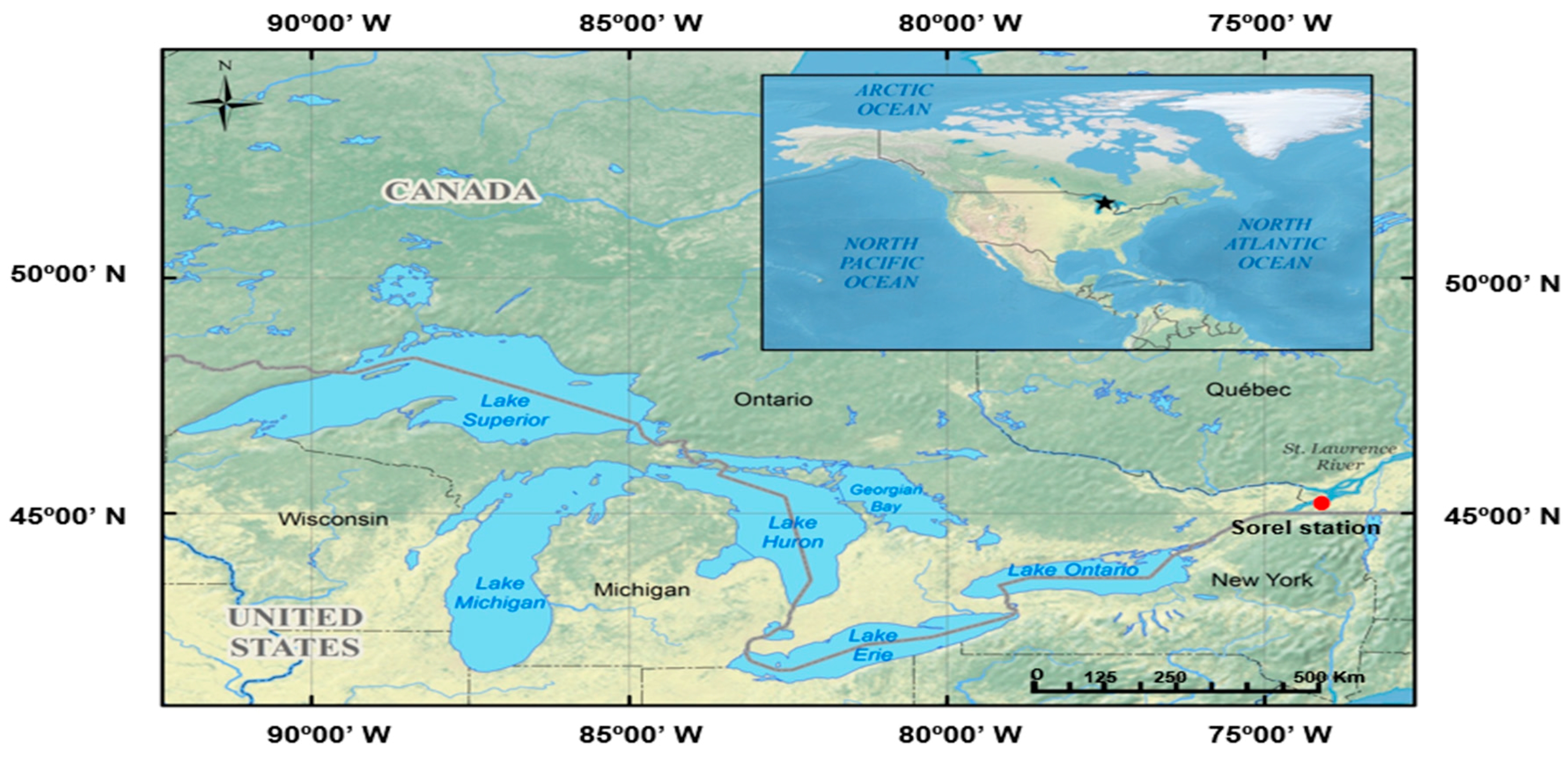
2.1. Study Sites and Source of Hydrological Data

The Great Lakes system comprises five great lakes, and thousands of smaller lakes, and the St. Lawrence River which is the natural outlet (Figure 1). Located between the United States and Canada, this aquatic system makes up one of the largest freshwater systems in the world. Covering 244,000 km², their watershed is home to roughly 30 million people (9% of the US population and 29% of the Canadian population) and holds 20% of the world’s freshwater reserves, for a total volume on the order of 23 × 10¹² m³. It plays a key role in the social and economic development of this region of North America and provides drinking water for domestic use, irrigation for agriculture, in addition to allowing commercial trade with other regions of North America and other continents, supplying hydroelectric power plants for energy production, and supporting recreational and tourism activities, as well as fishing [7].

This study is based on the analysis of monthly mean maximum and minimum water level data for the five Great Lakes (Superior, Michigan-Huron, Erie and Ontario) and St. Lawrence River measured from 1918 to 2012. The choice of these two hydrologic variables is predicated on their greater sensitivity to human activity than that of mean annual values of water levels [8,9]. These data were taken from [10]. It is important to note that precipitation, temperature and evaporation data were not analyzed as part of this study, as these data have already been analyzed by numerous authors [11,12,13]. They were, however, used to interpret changes in stationarity and dependence of water levels in the Great Lakes and St. Lawrence River. Finally, from a hydraulic standpoint, Lakes Michigan and Huron form a single system (Lake Michigan-Huron), and the temporal variability of their water levels is therefore identical. Thus, the term Lake Michigan-Huron is used in the remainder of this paper.

2.2. Statistical Analysis

Two statistical analyses were applied to monthly mean maximum and minimum water level data. The first consisted in detecting changes in mean and variance values of the hydrological series in order to correlate these changes to the various man-made structures built in the Great Lakes watershed. This was done using the Lombard method [14,15], which was selected because it allows the detection of both abrupt and gradual changes in mean and variance values, something that other tests commonly used in hydroclimatology cannot do [16]. In addition, this method is sensitive to small changes in mean and variance, unlike other tests [16]. Because the Lombard test equations have been presented in several papers (e.g., [16,17,18]), they are not described herein. According to this test, at the 95% confidence interval, one concludes that the mean or variance of the series changes significantly whenever S_n > 0.0403. This last value corresponds to the theoretical (critical) values [14] defining the significance level at 5% for the test. S_n is Lombard test value statistic calculated using the Lombard test from series of observation data. It is important to note that this test was applied to non-autocorrelated series (time-independent residuals).

The second statistical analysis was aimed at detecting changes in the dependence of water levels in the lakes and St. Lawrence River. It should be recalled that the five Great Lakes and the St. Lawrence River are connected with one another. Consequently, there is an interaction which causes the temporal variability of their water levels to be dependent. This analysis is therefore used to determine whether some of the man-made structures significantly modified the dependence between water levels. To this end, we applied the copula method, which is increasingly used in hydrology, consistent with the mathematical description offered in [15,19], among others. This method can detect sharp shifts in the dependence between two variables over time, these variables being, for this study, water levels in the lakes.

The method has been described in some of our previous work (e.g., [18,20]). The dependence in a random vector (X, Y) is contained in its corresponding copula function C. Specifically, the theorem of Sklar ensures that there exists a unique $C:{\left[0,1\right]}^2\to \left[0,1\right]$ such that

$$P\left(X\le x,Y\le y\right)=C\left\{P\left(X\le x\right),P\left(Y\le y\right)\right\}.$$

(1)

Quessy et al. [19] developed a testing procedure to identify a change in the copula (i.e., dependence structure) of a bivariate series $\left(X_1,Y_1\right),\dots ,\left(X_n,Y_n\right)$. The idea is based on Kendall’s tau, which is a nonparametric measure of dependence. Let ${\widehat{T}}_{1:T}$ be Kendall’s tau measured for the first Τ observations and ${\widehat{T}}_{T+1:n}$ be Kendall’s tau for the remaining $n-T$ observations. The proposed test statistic is

$$M_n={\text{max}}_{1<T<n}\frac{T\left(n-t\right)}{n\sqrt{n}}\left|{\widehat{T}}_{1:T}-{\widehat{T}}_{T+1:n}\right|$$

(2)

i.e., a maximum weighted difference between the Kendall’s tau. Since M_n depends on the unknown distribution of the observations, the so-called multiplier re-sampling method is used for the computation of p-values. Specifically, for $n$ sufficiently large (n > 50), this method yields independent copies $M_n^{(1)},\dots M_n^{(N)}$ of M_n. Then, a valid p-value for the test is given by the proportion of $M_n^{(i)}$’s larger than M_n. For more details, see Quessy et al. [19]. Usually, one can expect that the series X₁,…, X_n and Y₁,…, Y_n are subject to changes in the mean and/or variance following, e.g., the smooth-change model [14]. If such changes are detected, the series must be stabilized (to remove the shift of the mean and variance) in order to have (approximately) constant means and variances. Finally, a change in the degree of dependence between two series is statistically significant when M_n > V_c, where V_c is the critical value derived from observational data. As part of this study, the copula method was applied to standardized data for water levels in the lakes and St. Lawrence River after removal of shifts in mean and variance values in these hydroclimate data series.

3. Results

3.1. Analysis of Water Level Stationarity

Results obtained using the Lombard test analysis are presented in

Table 1. Lombard test results for monthly mean water levels in four North American Great Lakes over the period from 1918 to 2012. Analysis of mean values.

	Minimum			Maximum
	Sn	T1	T2	Sn	T1	T2
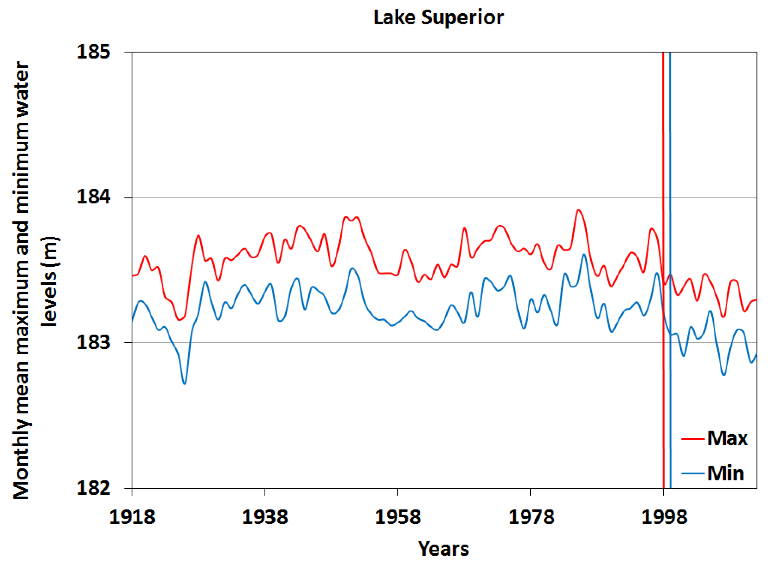
Lake Superior	0.0493	1998	1999	0.0627	1997	1998
Lakes Michigan-Huron	0.0204	-	-	0.0167	-	-
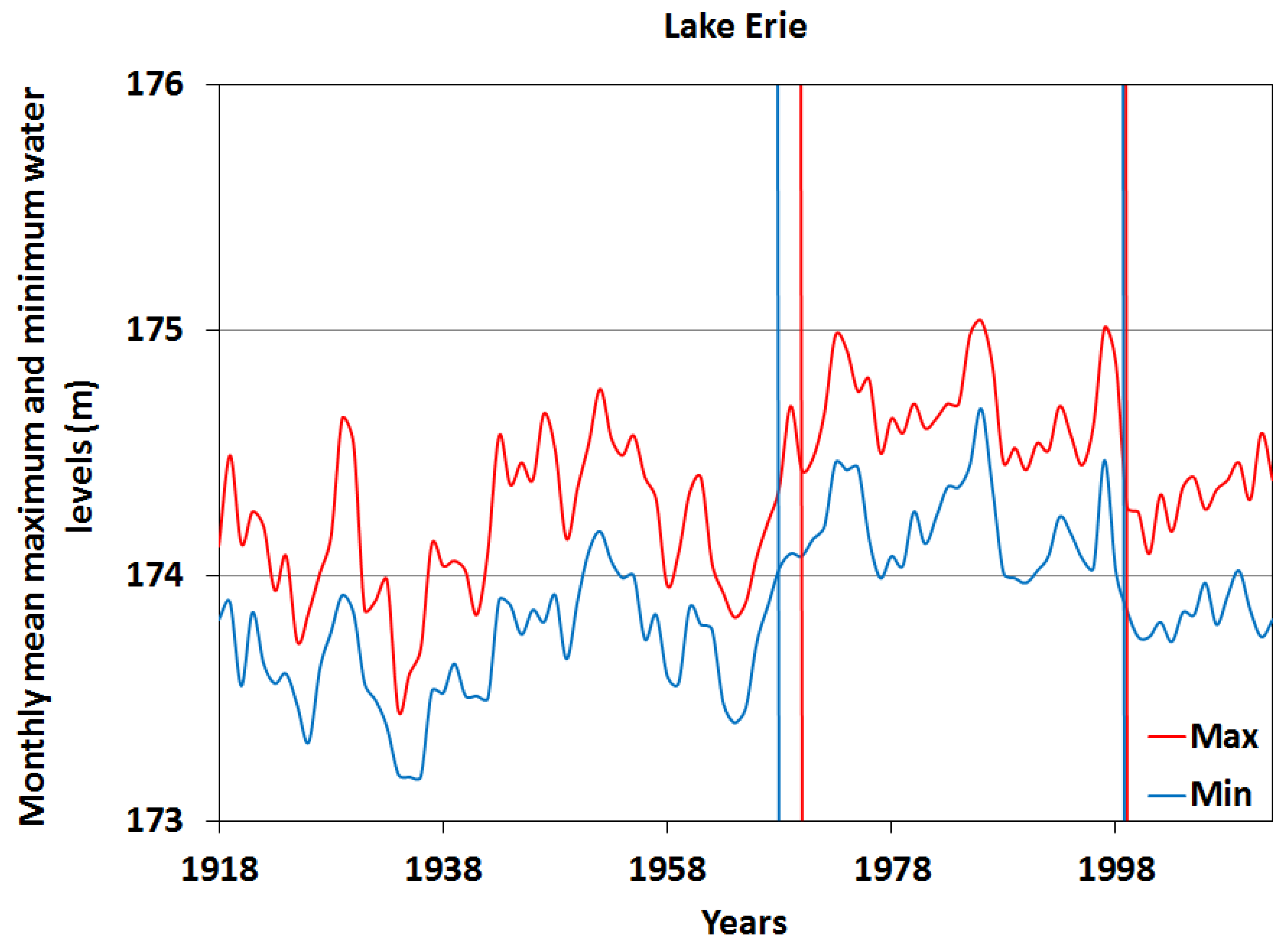
Lake Erie	0.2974	1966	1968	0.2300	1967	1970
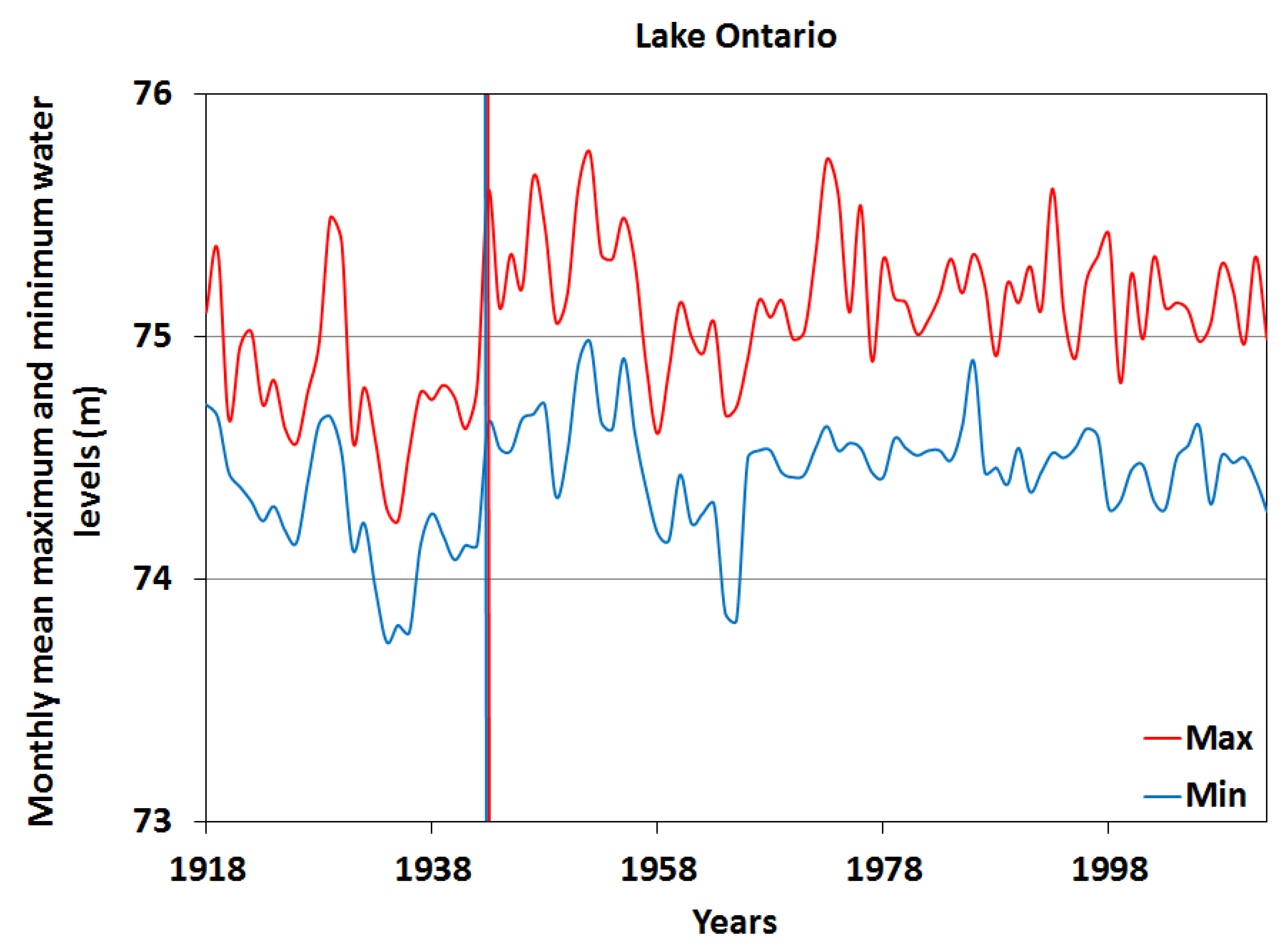
Lake Ontario	0.1236	1942	1943	0.0417	1942	1943
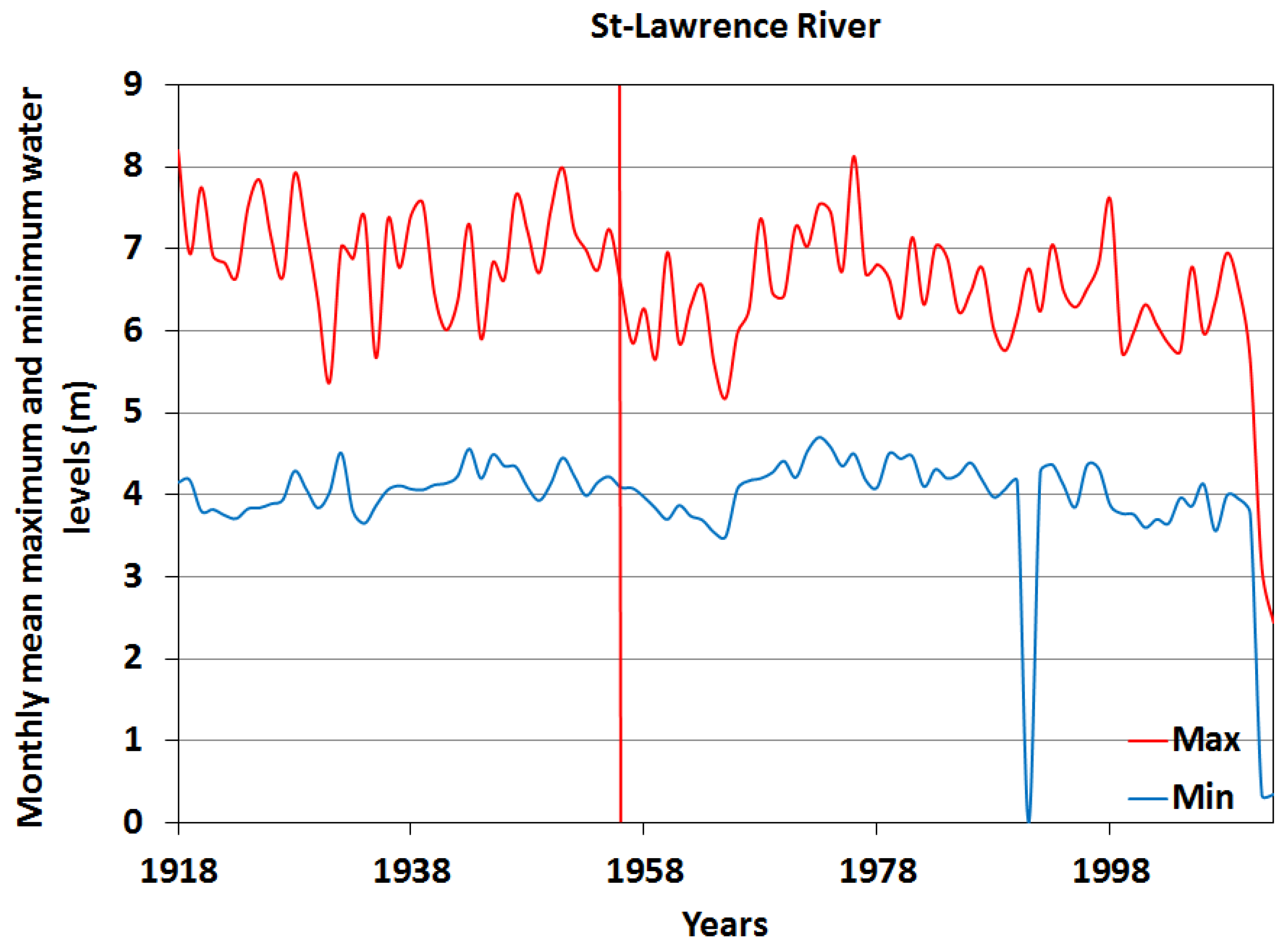
St. Lawrence River	0.0123	-	-	0.1042	1955	1956

Notes: Lombard test S_n values > 0.0403 are statistically significant at the 5% level. S_n = Lombard test value statistic. T1 and T2 are the years of start and end, respectively, of significant changes in mean and variance values of a given series.

and

Table 2. Lombard method results for monthly mean water levels prior and after the first shift.

Lake		Minimum			Maximum
	Periods	Sn	T1	T2	Sn	T1	T2
Superior	1918–1997	0.0201	-	-	0.0201	-	-
	1998–2012	0.0097	-	-	0.0286	-	-
Erie	1918–1965	0.0341	-	-	0.0276	-	-
	1969–2012	0.2262	1997	1999	0.1716	1998	1999
Ontario	1918–1941	-	-	-	0.0389	-	-
	1944–2012	-	-	-	0.0045	-	-
St. Lawrence	1918–1954	-	-	-	0.0063	-	-
	1957–2012	-	-	-	0.0104	-	-

Notes: Lombard test S_n values > 0.0403 are statistically significant at the 5% level. S_n = Lombard test value statistic. T1 and T2 are the years of start and end, respectively, of significant changes in mean and variance values of a given series.

and Figure 2, Figure 3, Figure 4, Figure 5 and Figure 6. For monthly mean minimum water levels, Lake Erie shows two shifts in mean values during the period from 1918 to 2012. The main shift, which is sharp, took place between 1966 and 1968. After this shift, mean values of the monthly mean minimum water levels increased significantly. This main shift was followed by another one which was just as sharp, between 1997 and 1999. After this shift, mean values of monthly mean minimum water levels decreased. A single sharp shift in mean characterizes monthly mean minimum water levels in Lakes Superior (in 1999) and Ontario (in 1943). No shift is observed for Lake Michigan-Huron and St. Lawrence River. In the case of Lake Superior, monthly mean minimum water levels decreased significantly after the shift, while for Lake Ontario, they increased significantly. As far as monthly mean maximum water levels are concerned, shifts in mean values occurred nearly synchronously with shifts in monthly mean minimum water levels for Lakes Superior, Erie and Ontario. In the St. Lawrence River, the sharp shift took place in 1956. No shift is observed for Lake Michigan-Huron. Finally, Lakes Superior and Ontario are the only lakes that show shifts in variance values (

Table 3. Lombard method results for monthly mean water levels in the North American Great Lakes over the period from 1918 to 2012. Analysis of variance values.

	Minimum			Maximum
	Sn	T1	T2	Sn	T1	T2
Lake Superior	0.0416	1996	1997	0.0245	-	-
Lakes Michigan-Huron	0.0233	-	-	0.0003	-	-
Lake Erie	0.0138	-	-	0.0286	-	-
Lake Ontario	0.2416	1965	1966	0.1962	1958	1959
St-Lawrence River	0.0161	-		0.0129	-	-

Notes: Lombard test S_n values > 0.0403 are statistically significant at the 5% level. S_n = Lombard test value statistic. T1 and T2 are the years of start and end, respectively, of significant changes in mean and variance values of a given series.

). For Lake Superior, this shift in variance occurred in 1997 for monthly mean minimum water levels, whereas for Lake Ontario, shifts occurred in 1959 and 1966, respectively, for monthly mean minimum and maximum water levels.

3.2. Analysis of Dependence Using the Copula Method

Results of the analysis of dependence, using the copula method, of water levels in the lakes taken in pairs are shown in

Table 4. Analysis of dependence between lakes monthly mean water levels. Results obtained using the copula method.

	Minimums				Maximums
	Mn	Vc	p-Values	T	Mn	Vc	p-Values	T
Superior-Michigan	0.6702	0.8763	0.1880	-	0.7651	0.8080	0.0730	-
Michigan-Erie	0.5418	0.5339	0.0430	1970	0.5209	0.5419	0.0670	-
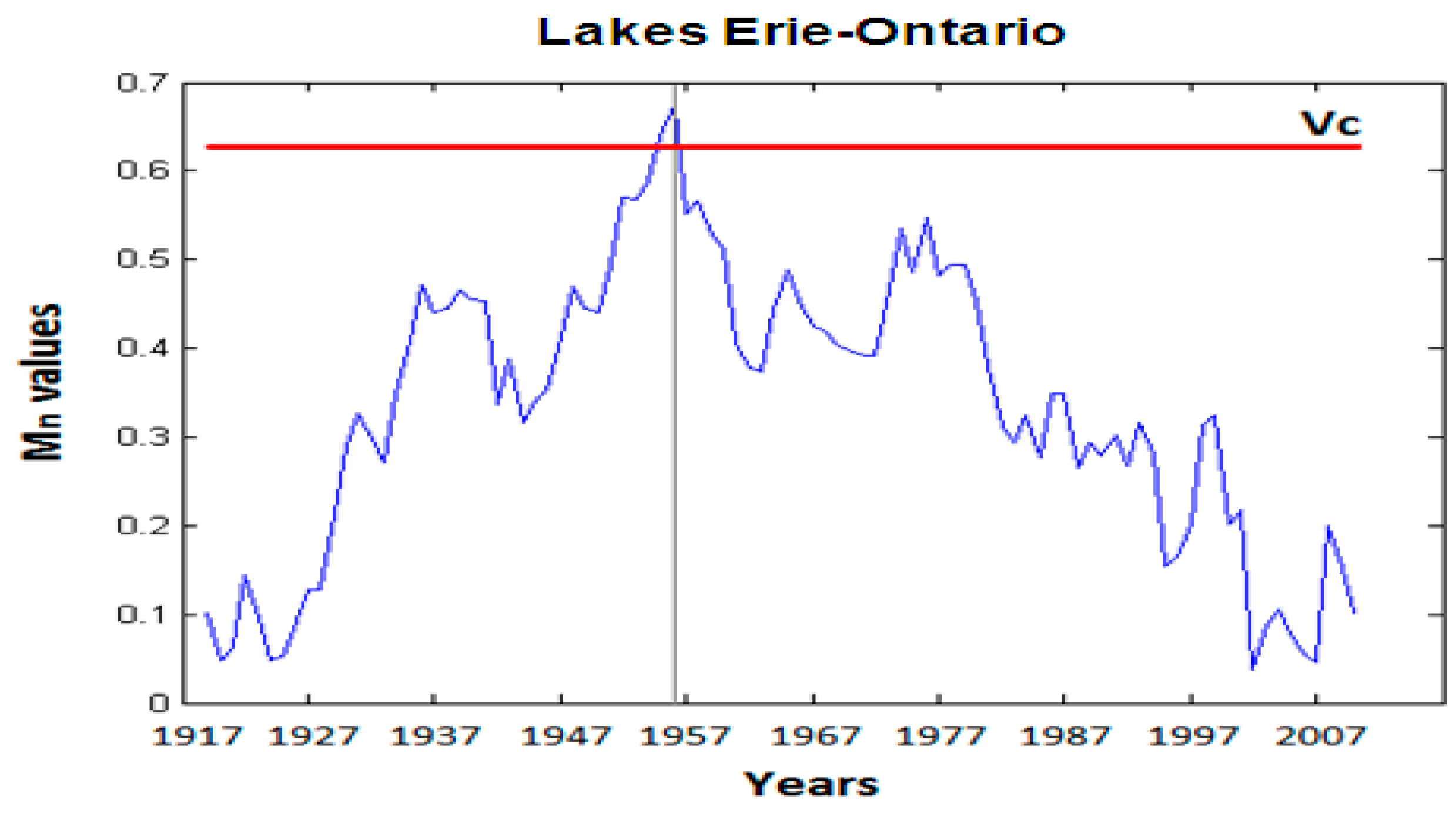
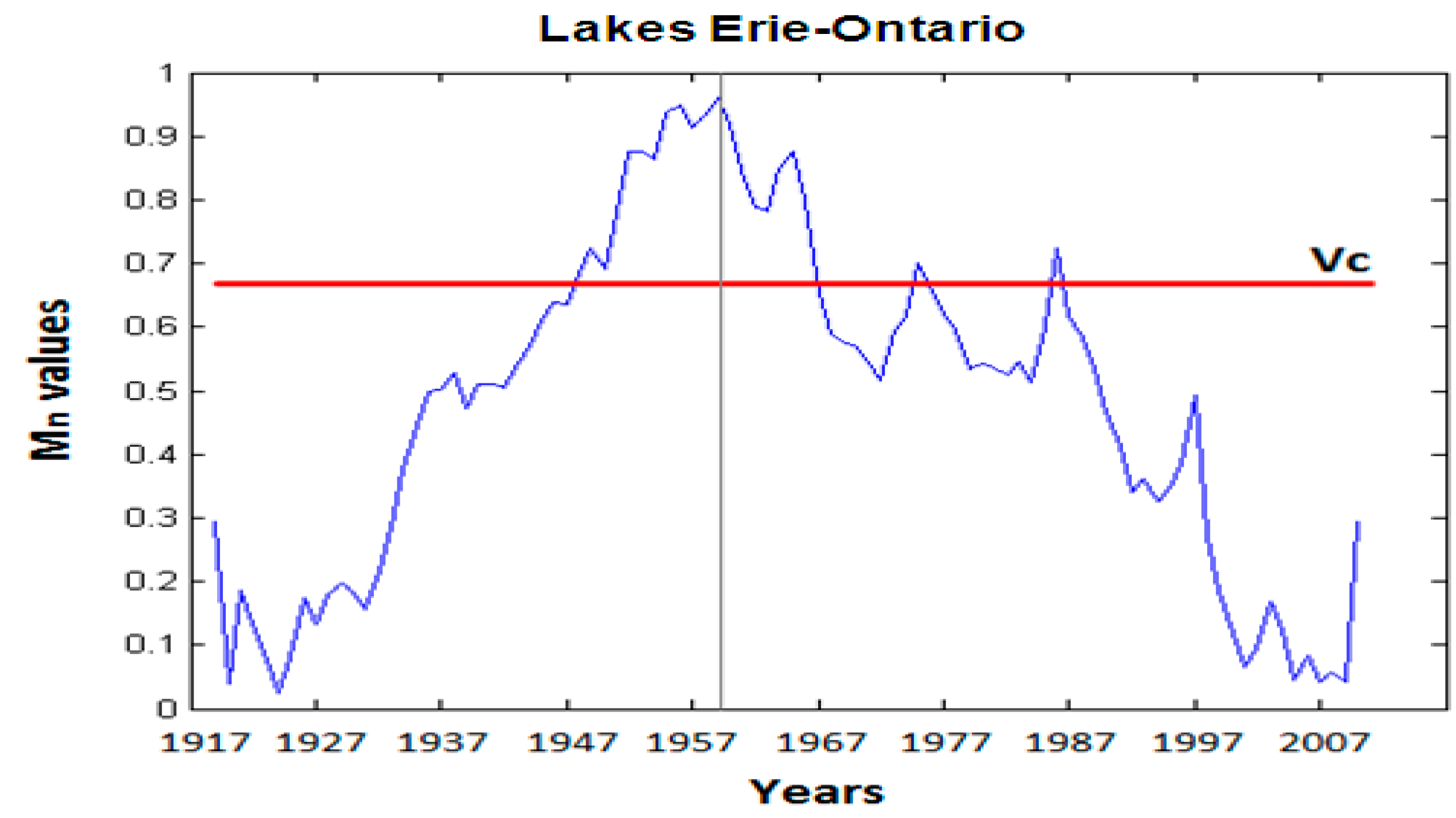
Erie-Ontario	0.9593	0.6690	0.0000	1958	0.6753	0.6278	0.0280	1956
Ontario-St.Lawrence	0.4620	0.8912	0.291	-	0.7641	0.7950	0.065	-

Notes: M_n = derived copula value; V_c = critical theoretical value; T = year of shift in dependence. Statistically significant M_n values at the 5% levels are shown in bold. Note: This is Lake Michigan-Huron.

. For monthly mean minimum water levels, a change in dependence is observed between water levels in Lakes Michigan-Huron and Erie (Figure 7), on one hand, and between water levels in Lakes Erie and Ontario (Figure 8), on the other hand. The former change occurred in 1970 and the latter in 1958. For monthly mean maximum water levels, a single change in dependence was detected, between water levels in Lakes Erie and Ontario (Figure 9). This change took place in 1956.

4. Discussion

The goal of the study was to constrain the impacts of man-made works on the stationarity (mean and variance) of monthly mean maximum and minimum water levels in the Great Lakes and St. Lawrence River on one hand, and on the evolution of their dependence on the other hand. Since the 19th century, many works have been built in the Great Lakes watershed, but the effects of these works on the various Great Lakes are not uniform, with large-scale water level regulation works mainly affecting Lakes Superior and Ontario, as well as the St. Lawrence River.

As far as stationarity is concerned, changes in mean and variance values did not affect the five Great Lakes in the same way, nor at the same time. For monthly mean minimum and maximum water levels, two shifts in mean values were detected for Lake Erie, while no shift was detected for Lake Michigan-Huron. These two lakes are the two Great Lakes least affected by water level regulation works. Thus, the temporal variability of their water levels is entirely determined by climate variability. It follows that shifts in the mean values of water levels in Lake Erie are caused by the succession of dry and wet periods in the Great Lakes watershed [6]. Analysis of precipitation and evaporation in the Great Lakes watershed reveals that the shift that occurred in the 1960s is linked with a large increase in precipitation while, unlike this first shift, the second shift that took place in the late 1990s cannot be linked to a substantial decrease in precipitation. It is rather interpreted to result from an increase in evaporation caused by higher water temperature due to decreasing ice cover in winter and fall (e.g., [11]). Although deeper, Lake Superior does show a shift in mean values at the end of the 1990s. This shift in mean is therefore interpreted to result from high evaporation due to the relatively strong warming of lake waters following a decrease in ice cover [21,22]. For instance, Austin and Colman [21] showed that water temperature in Lake Superior was increasing at a faster rate than the air temperature, resulting in enhanced evaporation. The absence of a shift in the mean values of monthly mean maximum and minimum water levels in Lake Michigan-Huron, despite the fact that it is less deep than Lake Superior, might suggest that water warming causing intense evaporation was less extensive in Lake Michigan-Huron than in Lake Superior. In addition, this absence of shifts in mean and variance was also observed in annual mean water levels in this lake [6]. Although Lake Ontario water levels are highly regulated as a result of the digging of the St. Lawrence Seaway during the 1950s, the shift in the mean values of monthly mean minimum water levels in this lake took place in the 1940s, before Seaway construction, and is the result of increased precipitation in the wake of the Great Drought of the 1930s. In contrast, the shift in variance of monthly mean maximum and minimum water levels occurred after the digging of the Seaway, this variance decreasing significantly over time due to water level regulation following the construction of dams and locks. The shift in mean values of monthly mean maximum water levels in the St. Lawrence River, which occurred in 1956, may be linked with the digging of the Seaway.

As far as dependence is concerned, a significant change is observed between monthly mean minimum and maximum water levels in Lakes Erie and Ontario that took place during the digging of the St. Lawrence Seaway. The most recent change in dependence was observed in 1970 between monthly mean minimum water levels in Lakes Michigan-Huron and Erie. This change in dependence between the two lake systems could be mainly accounted for by the significant increase in water levels in Lake Erie that occurred after 1970 (the two main shifts in mean water levels in Lake Erie occurred in 1968 for monthly mean minimum water levels and 1970 for monthly mean maximum water levels, see Table 1), a situation not observed for Lake Michigan-Huron, where water levels show no increase or decrease after that year. The effects of climate-induced changes in water levels in Lake Erie on the dependence of water levels between the two lake systems were likely amplified by dredging work carried out in the St. Clair and Detroit Rivers in 1970, which was followed by a significant increase in the depth of these two rivers. It would be interesting to constrain the relative influence of these two factors (climate variability and dredging) on this change in dependence of water levels in these two lakes.

5. Conclusions

This study highlights several shifts in mean and variance values of monthly mean maximum and minimum daily water levels for some of the Great Lakes and their natural outlet, the St. Lawrence River. These shifts are interpreted to be caused primarily by climate variability, with man-made works having had very little effect on the stationarity and dependence of water levels. The impacts of these works mainly resulted in a decrease in variance of water levels in Lake Ontario and of monthly mean maximum daily water levels in the St. Lawrence River after digging of the St. Lawrence Seaway on one hand, and a change in the dependence between water levels in Lakes Ontario and Erie on the other hand. The analysis did not bring out any impact of water level regulation on the stationarity and dependence of water levels in Lake Superior. In light of these results, the various works constructed since the 19th century have had a limited impact on the temporal variability of monthly mean maximum and minimum water levels in the Great Lakes and St. Lawrence River.

References

- Clites, A.H.; Quinn, F.H. The history of Lake Superior regulation: Implications for the future. J. Gt. Lakes Res. 2003, 29, 157–171. [Google Scholar] [CrossRef]
- Lee, D.H.; Quinn, F.H.; Sparks, D.; Rassam, J.C. Modification of great lakes regulation plans for simulation of maximum Lake Ontario outflows. J. Gt. Lakes Res. 1994, 20, 569–582. [Google Scholar] [CrossRef]
- Quinn, F.H. Lake Superior regulation effects. Water Resour. Bull. 1978, 14, 1129–1142. [Google Scholar] [CrossRef]
- Quinn, F.H. Anthropogenic changes to Great Lakes water levels. Gt. Lakes Update 1999, 136, 1–4. [Google Scholar]
- Assani, A.A.; Landry, R.; Stacey, B.; Frenette, J.J. Analysis of the interannual variability of annual daily extreme water levels in the St. Lawrence River and Lake Ontario from 1918 to 2010. Hydrol. Process. 2014, 28, 4011–4022. [Google Scholar] [CrossRef]
- Assani, A.A.; Landry, R.; Azouaoui, O.; Massicotte, P.; Gratton, D. Comparison of the characteristics (frequency and timing) of drought and wetness indices of annual mean water levels in the five North American Great Lakes. Water Resour. Manag. 2016, 30, 359–373. [Google Scholar] [CrossRef]
- Magnuson, J.J.; Webster, K.E.; Assel, R.A.; Bowser, C.J.; Dillon, P.J.; Eaton, J.G.; Evans, H.E.; Fee, E.J.; Hall, R.I.; Mortsch, L.R.; et al. Potential effects of climate changes on aquatic systems Laurentian Great Lakes and Precambrian Shield Region. Hydrol. Process. 1997, 11, 825–871. [Google Scholar] [CrossRef]
- Assani, A.A.; Gravel, E.; Buffin-Bélanger, T.; Roy, A.G. Impacts of dams on the annual minimum discharges according to artificialized hydrologic regimes in Quebec (Canada). J. Water Sci. 2005, 16, 103–127. (In French) [Google Scholar]
- Assani, A.A.; Stichelbout, E.; Roy, A.G.; Petit, F. Comparison of impacts of dams on the annual maximum flow characteristics in three regulated hydrologic regimes in Quebec (Canada). Hydrol. Process. 2006, 20, 3485–3501. [Google Scholar] [CrossRef]
- Government of Canada. Fisheries and Oceans. Historical Monthly and Yearly Mean Water Level 1918–2013. Available online: http://tides.gc.ca/C&A/historical-eng.html (accessed on 26 November 2013).
- Assel, R.A.; Quinn, F.H.; Sellinger, C.E. Hydroclimatic factors of the recent record drop in Laurentian great lakes water levels. Bull. Am. Meteorol. Soc. 2004, 85, 1143–1151. [Google Scholar] [CrossRef]
- Gronewold, A.A.; Fortin, V.; Logfren, B.; Clites, A.; Stow, C.A.; Quinn, F. Coasts, water levels, and climate change: A Great Lakes perspective. Clim. Chang. 2013, 120, 697–711. [Google Scholar] [CrossRef]
- McBean, E.; Motiee, H. Assessment of impact of climate change on water resources: A long term analysis of the Great Lakes of North America. Hydrol. Earth Syst. Sci. 2008, 12, 239–255. [Google Scholar] [CrossRef]
- Lombard, F. Rank tests for changepoint problems. Biometrika 1987, 74, 615–624. [Google Scholar] [CrossRef]
- Quessy, J.-F.; Favre, A.-C.; Saïd, M.; Champagne, M. Statistical inference in Lombard’s smooth-change model. Environmetrics 2011, 22, 882–893. [Google Scholar] [CrossRef]
- Villarini, G.; Smith, J.A.; Serinaldi, F.; Ntelekos, A.A. Analyses of seasonal and annual maximum daily discharge records for Central Europe. J. Hydrol. 2011, 399, 299–312. [Google Scholar] [CrossRef]
- Assani, A.A.; Landry, R.; Daigle, J.; Chalifour, A. Reservoirs effects on the interannual variability of winter and spring streamflow in the St. Maurice River Watershed (Quebec, Canada). Water Resour. Manag. 2011, 25, 3661–3675. [Google Scholar] [CrossRef]
- Mazouz, R.; Assani, A.A.; Quessy, J.-F. Comparison of the interannual variability of spring heavy floods characteristics of tributaries of the St. Lawrence in Quebec (Canada). Adv. Water Resour. 2012, 35, 110–120. [Google Scholar] [CrossRef]
- Quessy, J.-F.; Saïd, M.; Favre, A.-C. Multivariate Kendall’s tau for change-point detection in copulas. Can. J. Stat. 2012, 40, 1–18. [Google Scholar] [CrossRef]
- Guerfi, N.; Assani, A.A.; Mesfioui, M.; Kinnard, C. Comparison of the temporal variability of winter daily extreme temperatures and precipitations in southern Quebec (Canada) using the Lombard and copula methods. Int. J. Climatol. 2015, 35, 4237–4246. [Google Scholar] [CrossRef]
- Austin, J.; Colman, S. Lake Superior summer water temperature are increasing more rapidly than regional air temperature: A positive ice-albedo feedback. Geophys. Res. Lett. 2007, 34, L06604. [Google Scholar] [CrossRef]
- Van Cleave, K.; Lenters, J.D.; Wang, J.; Verhamme, E.M. A regime shift in Lake Superior ice cover, evaporation, and water temperature following the warm El Nino winter of 1997–1998. Limnol. Oceanogr. 2014, 59, 1889–1898. [Google Scholar] [CrossRef]