1. Introduction
Mining is common in many African countries and it brings substantial revenues to the governments. However, development of mining activities may seriously impact the environment [
1]; thus, water quality is one issue that has to be carefully addressed in the context of mining [
2,
3,
4,
5,
6,
7].
Mining is growing, the impacts are imminent, and the water quality monitoring programs in developing countries are not well established to assess the water quality changes [
8]. A lack of resources is one of the main constraints in implementing sustainable water quality monitoring programs in developing countries [
8]. This makes it important to develop less resource-demanding monitoring programs supported by mathematical models that minimize the required sampling and analysis, while retaining the capability to detect and quantify water quality changes, thereby allowing for the rapid implementation of measures to protect water resources.
There are a number of existing mathematical models that may be useful in connection with water quality monitoring programs, the most common being the Streeter–Phelps model, the QUAL Model, WASP Models, QUASAR Model, MIKE Models, BASIN Model, EFDC Model, and PHREEQ C [
9]. However, none of these models were developed specifically to deal with water quality evolution in rivers affected by mining. The models also require a lot of input data to perform simulations, while such data are not readily available in most developing countries.
The pH is of great importance in establishing the degree of contamination in rivers impacted by mining. This is because one of the well-known problems of mining is Acid Mine Drainage (AMD), which is produced when pyrite is exposed to air and water. Hence, it is useful to develop a model based on pH because it affects the concentrations of different ions in the water by influencing the solubility of minerals [
10]. Besides influencing the solubility of minerals, the pH also directly impacts life in aquatic systems [
11].
There are relatively few studies about concentration changes of major ions (MI) in rivers compared to minor ions and heavy metals. A thorough search of the literature by the authors of this study did not reveal any studies that include models to estimate the concentrations of MI in rivers. Although rather old, an interesting inventory of the concentrations of MI in rivers and lakes all over the world was carried out in the context of salt discharge to the oceans [
12]. The study resulted in an estimate of the total amount of salts discharged to the oceans by rivers and the average concentrations of MI in rivers per continent [
12,
13,
14,
15].
In this paper, a new, simplified mathematical model is presented that can estimate the concentration of MI in rivers affected by mining and other activities that influence the speciation of ions in water. The model is based on the input of pH, alkalinity, and temperature only. It is also shown that the model can be extended to incorporate other important parameters such as concentration of minor ions and heavy metals using the theory of solubility of minerals.
This model is useful when the aim is to obtain a general picture of the concentration of MI, some minor ions, and heavy metals in water in regions where there is lack of resources to do detailed monitoring and analysis. The main strategy in the present model development is to minimize the number of input parameters, thereby making the model easy to use when information is scarce and resources are limited.
2. Methods
The model was developed based on a review of relevant literature and data together with existing chemical models and theories that relate concentrations of different ions in river water to pH, alkalinity, temperature, and electric conductivity. These parameters were selected because they are rather easy to measure and can be determined in the field at low cost. The outcome of this review resulted in a mathematical model that was formulated and solved using a computer code implemented in the Fortran and Python programming languages. Subsequently, the model was tested by comparing predictions with recorded data at four monitoring stations in Swedish rivers. The selection of the Swedish rivers was justified by the availability of comprehensive data covering a long period of time. Although the focus of the present study was to develop a method to be applicable in developing countries, the governing laws for equilibrium concentration are universal and not site specific, which implies that a comprehensive data set from any river is suitable for testing the model. However, with regard to data availability, the model was formulated with two options: The first option, denoted as the generalized method, employs existing continental averages for the concentrations of MI in the database of the model and can be employed to get a first estimate of the concentration of MI in rivers without local data. The second model option, denoted as the customized method, requires the user to input local data on concentrations to tune the model to the specific conditions.
The theoretical concepts and relationships employed to develop this model are: (i) carbonate equilibrium; (ii) total alkalinity; (iii) statistics of MI; (iv) solubility of minerals; and (v) conductivity as function of MI in water.
2.1. Theory
In this section the different theories and concepts used to develop the model are reviewed. The model is developed to be used for freshwater that has a low concentration of total dissolved solids (TDS). The activity coefficients of chemical species in freshwater are close to one and, to simplify the approach, the molar concentration of an ion is assumed to be equal to its activity. This restricts the applicability of the model to freshwater, which is a reasonable hypothesis given that the TDS in rivers is generally low. For this modelling, water that has TDS or electrical conductivity below 1000 mg/L or 1500 μS/cm, respectively is considered freshwater [
16,
17].
(i) Carbonate equilibrium
The carbonate equilibrium is directly related to pH and alkalinity of water; thus, it is important to include the chemistry of carbonates to model pH and associated parameters. The equilibrium of carbonic acid is defined by Equations (1)–(4) [
10].
The equilibrium constants are dependent on temperature and there are several models developed to describe these dependencies. The models given by Equations (5) and (6) can be found in [
10].
(ii) Total alkalinity
Alkalinity is defined as the ability of water to neutralize acids. It expresses the excess of proton acceptors over proton donors. Total alkalinity (
TA) is given by Equation (7) [
18].
The total alkalinity can be determined with a higher accuracy using equations that are more complex than Equation (7), since the ability to neutralize acids does not depend only on the concentrations of ions included in this equation. There are many other ions competing to neutralize acids [
18]. However, for the purpose of the modelling here, Equation (7) is sufficient.
(iii) Major ions in water
Major ions in natural waters are the ones that usually appear in significantly larger concentrations compared to others. In surface water the most common major ions are:
Na+, K+, Mg2+, Ca2+,
HCO3−,
SO42−,
Cl−, and
NO3− [
15]. The average concentrations of each of these ions in rivers per continent are given in
Table 1 in mg/L (ppm). There are several sources of uncertainty affecting the estimated average concentrations. The main sources of uncertainty are the limited number of samples in space (rivers) and time, that the estimates are based on [
12]; as well as the variability in the concentrations of MI in rivers of the same continent. The uncertainty, and its implications for the variability per continent, was not estimated in [
12]. Nevertheless, the data is used when there is no river specific baseline data available to calibrate the model. The uncertainty associated with the average concentrations is estimated and discussed in
Section 2.2.
(iv) Solubility of minerals
The solubility of minerals is determined by the solubility constants, here illustrated through an example for the following hypothetic mineral (
AB2). Equations (8) and (9) give the chemical reaction and the equation for the solubility constant of the mineral, respectively [
10].
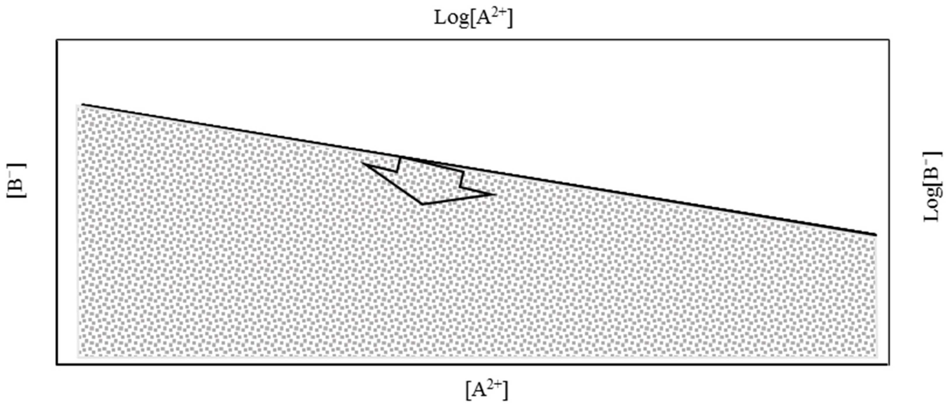
A comprehensive analysis of Equation (9) can be carried out by linearizing it (Equation (10)) and presenting the equation graphically (see
Figure 1).
In Equation (10),
b is a constant that depends on the solubility of the mineral. When the concentrations of
A2+ and
B− are presented graphically, as shown in
Figure 1, two domains appear: the super-saturated area in white and the non-saturated area (in grey) separated by the saturation line. In natural waters, the concentration of
A2+ and
B− should correspond to points in the non-saturated area or on the saturation line. When the concentration of one ion in the solution is known, the maximum possible concentration of the other ion can be estimated from the equilibrium concentration, because higher concentrations will lead to precipitation.
Solid phases and the solubility constants in
Table 2 were included in the model. More solid phases can be added to this list; these were selected to demonstrate the possibility of extending the model to estimate the concentration of ions at low concentration. A detailed study about the most relevant soluble phases, and more accurate solubility constants are necessary for further development of the model.
(v) Conductivity factors
There are quite complex methods to find the relationship between ion concentrations and electric conductivity in water. Some methods consider infinite dilution equivalent conductivity. This assumption allows the consideration that there is no pairing when oppositely charged ions are closer than a certain critical distance to make them act as a neutral molecule and hence they do not contribute to conductivity. However, assuming that there is no interaction between the molecules introduces uncertainty to the electro-conductivity estimated using this method. The electric conductivity calculated in this way lies within ±2% of experimentally determined values [
20]. The most complex and accurate methods include this effect [
21]. The main purpose of all these methods is to obtain conductivity factors of ions in water in [(μS/cm)/(mg/L)] to relate the concentration of single ions to the electric conductivity of water [
20]. The conductivity factors of ions commonly found in water are given in
Table 3.
The electric conductivity can be estimated using the concentrations (
Ci) and conductivity factors (
fi) of the ions present in water employing Equation (11).
The estimated conductivity will be used to indicate the overall accuracy of the model, see
Section 2.4.
2.2. Variation of Major Ions in Rivers
The first assumption made in the model development is that, considering only the MI, the concentration of positive ions and negative ions are in balance. This means that the sum of the concentrations of positive ions in meq/L is equal to the sum of the concentrations of negative ions considering only the MI. This assumption has to be verified before being used in the model. In the first step, to perform this verification, the average concentrations of ions in river waters in mg/L given in
Table 1 are converted to meq/L, see
Table 4; this allows for a charge balance between positive and negative ions. The concentrations are further converted into a percentage of each ion in relation to the total concentration of positive ions in the case of a positive ion, and in relation to the total concentration of negative ions in the case of a negative ion (
Table 5), to be subsequently used in the modelling.
Ideally the difference between the total concentration of positive and negative ions in meq/L should be zero, considering the electro-neutrality of water. Assuming that the MI are the only ions present in river waters, for the different continents, the difference between the positive and negative ions is less than 7% for all continents except Australia. The difference between the total concentration of positive and negative ions reflects the presence of ions other than the major ones. Thus, it is reasonable to assume that the concentration of positive and negative ions in meq/L are equal for all continents, except Australia, and this assumption is employed in the model. A more general case was also evaluated based on world averages. The use of world averages will be discussed in more detail in a later section of the paper.
The model will use average relative concentrations in percentage to estimate the concentrations of MI in rivers. These averages are made available per continent in the model, and are used as default values, see
Table 5. A more accurate version of the model denoted as the “customized method” uses average values based on measured data from the specific river being modelled.
As stated before, the average concentrations used are affected by uncertainty. This uncertainty is due to many factors, such as the spatial and seasonal variability of the concentrations of ions on the same continent. Using data from [
12] it was possible to estimate the standard deviation of the relative concentrations of ions per continent. Assuming that the relative concentrations follow a normal distribution, using a confidence level of 90%, the variability in MI around the estimated averages was calculated and given in
Table 6. The variability of ions is quite large ranging from about ±1% for nitrate concentration in Asia to ±33% for chlorine concentration in Australia. There are cases where the average relative concentration is very low, but its variability is large. That is the case for the concentration of nitrate in North America, which is 0.9 ± 5.5%. However, it does not mean that it is possible to get a negative concentration of nitrate, but if a measurement of the concentration of nitrate is carried out in a stream in North America there is a 90% probability of obtaining a value between 0 and 6.4% in relation to the sum of the concentrations for nitrate, chlorine, sulphate, and hydrogen carbonate in eq/L. Considering the average concentrations given in
Table 1 and
Table 4, the concentration of nitrite is equivalent to the ranges 0 to 0.119 meq/L and 0 to 28.3 mg/L, respectively.
The second main assumption made in the model development is that the relative concentrations do not change over time. This assumption about the relative stability of the concentrations (as a percentage) of major ions in
Table 5 over time was also investigated in detail. The data from four monitoring stations in Swedish rivers was used to evaluate temporal changes in the relative MI concentrations. Since the model was developed to be used in major rivers, the selected stations have large upstream catchment areas: Skellefte älv, Slagnas (6460 km
2), Vindelälven, Maltbrännan (9900 km
2), V. Dalälven, Mockfjärd (8493 km
2), and Klarälven, Edsforsen (8580 km
2) [
22].
Unfortunately, it was difficult to find high-quality data from other countries, but it is expected that such data will display similar behavior as the Swedish data. This is an assumption to be investigated in future studies.
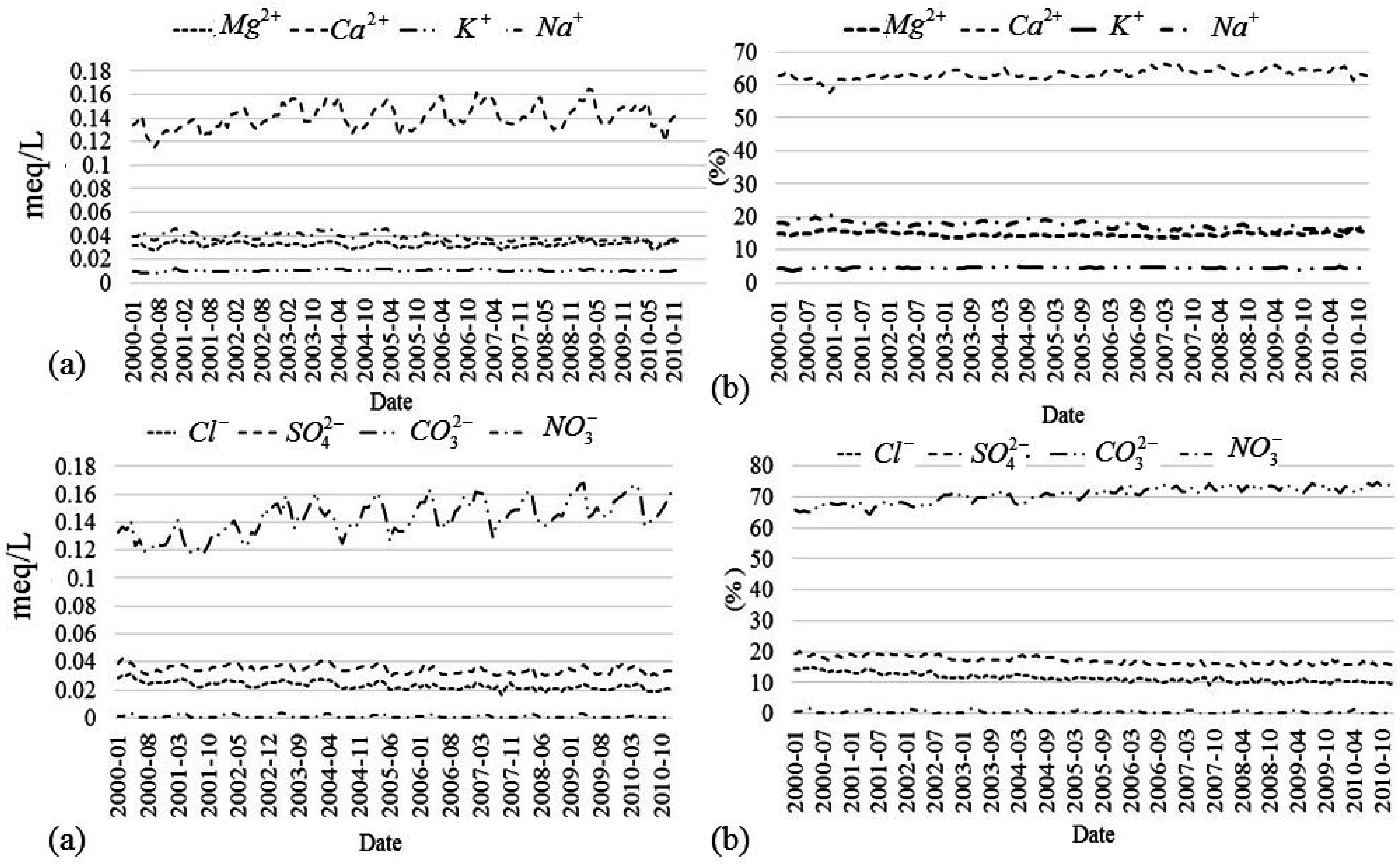
Data covering the period from 2000 to 2010 were used to analyze the temporal variations in the concentrations of
Mg2+,
Ca2+,
Na+,
K+,
HCO3−,
Cl−,
SO42−, and NO
3−. As a representative example, the data collected at Slagnäs station in Skellefte älv are shown in
Figure 2. The concentrations of these ions in meq/L show significant variability between the different seasons of the year, see
Figure 2a. However, this variability is always around an average value that exhibits a negligible trend, see
Table 5. The variability in the concentrations is caused by the seasonal variations in the catchment runoff and associated river flow. The relative concentrations expressed as a percentage (
Figure 2b) show less variability around the average values. This is because the concentrations of the different ions co-vary, making the relative concentration, as a percentage, less sensitive to seasonal changes.
The same behavior was found in the data from the other three stations, see
Table 6. The Mann–Kendall test (H) was used to evaluate the trend of the time series. The test was performed with a significance level of 0.05. The result is that, in most cases, there is enough evidence to say that there is no trend, (H = 0); however, in some cases, a trend (H = 1) cannot not be excluded at this significance level, see
Table 6. Linear regression was used to calculate the slope of the time series for the four monitoring stations selected for the study. The trending slopes of the time series are small; when evaluating the change in average relative concentration as a percentage (ΔC) over the 10 years studied (2000–2010) it is negligible compared to the average concentration.
The concentration of HCO3− shows a small positive trend, while the other anions show negative trends for the four stations. The average concentration of Ca2+ increases over time, while Mg2+ decreases and the other positive ions show different trends for the four stations. However, the trends found are small enough not to invalidate the assumption of constant relative concentrations of those ions over time and therefore the model can be used for practical applications. The trends may not be the same in all rivers over the world, but are likely to be small enough for model applications in many cases, since the concentrations depend mainly on the geology, which does not change over the typical engineering time scale, unless there is a marked human influence.
2.3. Model Algorithm
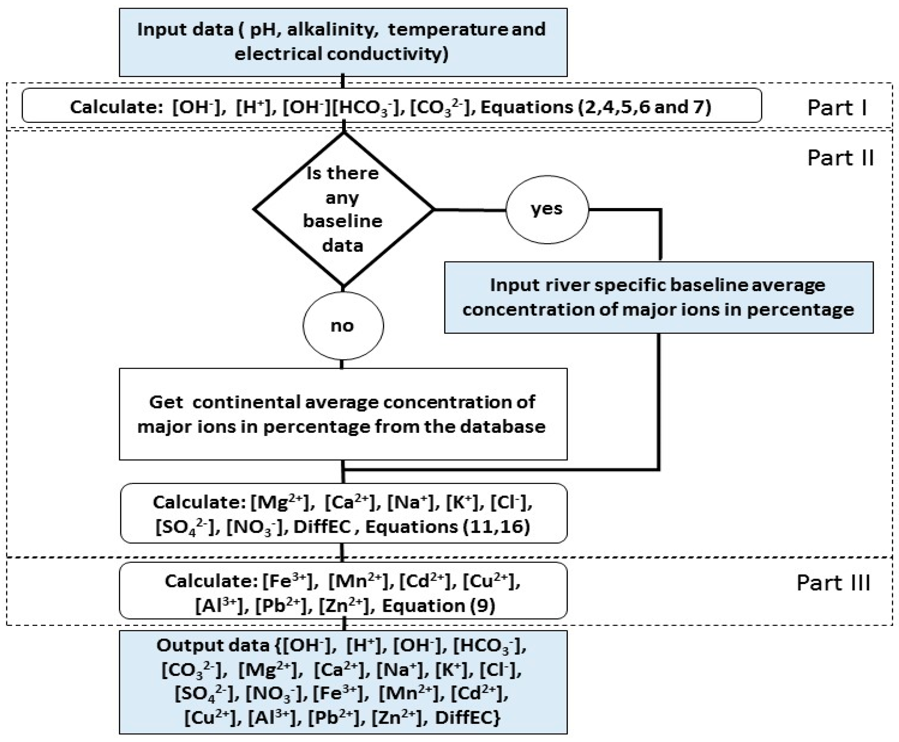
The model is divided into three parts, see
Figure 3.
In the first part, the model uses pH, alkalinity, and temperature to estimate the concentrations of H+, OH−, CO32−, HCO3−, and H2CO3.
In the second part, the concentrations of Ca2+, Mg2+, Na+, K+, HCO3−, Cl−, NO3−, and SO42− are estimated by the model from the concentration of HCO3− and the relative concentrations in (meq/L) in the database of the model for the generalized method or baseline-data for the customized method. Baseline data are the data of relative concentrations of MI necessary to calibrate the model. The relative concentrations are the major sources of error in the model, since it may change over time, as discussed above. The generalized method is an option that uses the default relative concentrations per region (Africa, North America, South America, Europe, Asia, Australia, or the “world”) in case there is no data on relative concentrations for the modelled river. The option “world” in the generalized method can be used for any region and it is possible to determine which option (regional or world) is giving better estimates by comparing the difference between estimated and measured electric conductivity [DiffEC(%)]. The model also estimates the total hardness as the sum of the concentrations of Ca2+ and Mg2+.
The
generalized method, which uses the continental averages, is to be employed only in cases where there are no possibilities to obtain specific river baseline data for model calibration, because it has the uncertainty associated with the continental averages in
Table 1, as discussed before. Since the
customized method does not use these averages, the estimated values will not be affected by this uncertainty. The estimated values using the
customized method will be affected by the uncertainty in the data used to calibrate the model and the assumption made that the only ions present in water are the MI. This uncertainty can be estimated for specific river data. However, a clue about the magnitude of this uncertainty is indicated for different continents and it is most likely to be large in Australia, and smaller for other continents because there is a significant difference between the sum of the concentrations of positive and negative ions in meq/L considering only the MI in Australia compared to other continents, see
Table 4.
In the third part of the model, the equilibrium equations are used to estimate the concentrations of iron, manganese, and some heavy metals using the equilibrium equations. The equilibrium constants used for the modelling are given in
Table 2. The main purpose of estimating heavy metals is to obtain maximum possible concentrations in order to decide whether there is a need for going to the field to take samples for more accurate analyses.
The overall mathematical formulation of the model is given by Equation (12).
where
T and
Alk are temperature and alkalinity, respectively.
In summary, the main input parameters are pH, alkalinity, and temperature, whereas measured conductivity may be used to estimate the error of the estimated results. Changes in the concentration of ions due to variation of flow caused by natural hydrological runoff are captured by the measured pH and alkalinity used as input parameters. Changes in the concentration of ions due to changes in the flow of contributing, contaminated streams, are more difficult to capture, and might lead to errors in the concentrations estimated by the model. These errors will, however, be detected by analyzing the magnitude of the
DiffEC variable, which is included in the model and discussed in
Section 2.4. The calculation method can be selected as general or customized. When the generalized method is selected, it is necessary to choose the continent where the river is located. If the customized method is selected, then it is necessary to input the relative concentrations of MI for the base month (or year) as a percentage, for the river to be modelled.
2.4. Evaluation of the Model Performance
(i) Difference between the measured and estimated electric conductivity as a percentage DiffEC(%)
In order to quantify the overall accuracy of the model, a parameter called
DiffEC(%) was introduced in the model. This parameter is the difference between the measured and estimated electric conductivity as a percentage, Equation (13).
Ideally, if all ions were included in the model, this value should be zero; however, the model estimates the electric conductivity using only the MI. The value should therefore always be higher than zero, because some ions are left out in the model. Sometimes the model may get DiffEC(%) less than zero, implying that it is underestimating the concentrations of ions with low electric conductivity factors (bicarbonate, sulfate, nitrate or potassium) or overestimating the ions with high electric conductivity factors (magnesium, calcium, chlorine or sodium). Even if the concentrations of ions with high electric conductivity are overestimated, the DiffEC(%) may still be positive when the concentrations of the ions not considered by the model are high.
When there is baseline data, the customized method can be used to estimate the concentrations of ions, and the value of DiffEC(%) for the base month (or the month in which data was collected to calibrate the model) should be higher than zero. The DiffEC(%) for the base month shows the relationship between the MI and the ions not considered by the model.
(ii) Root mean square error (RMSE)
To compare the modelled and the measured concentration values, the
root-mean-square error (
RMSE) was used, Equation (14).
where,
is the measured concentration of ions,
is the modelled value of the concentration and
is the number of samples used to evaluate the model.
The other parameters to quantify the error shown in
Table 5 are
RMSE min(%) and
RMSE max(%), which are
RMSE compared to the minimum and maximum measured value (as a percentage) (see Equations (15) and (16), respectively).
3. Results and Discussion
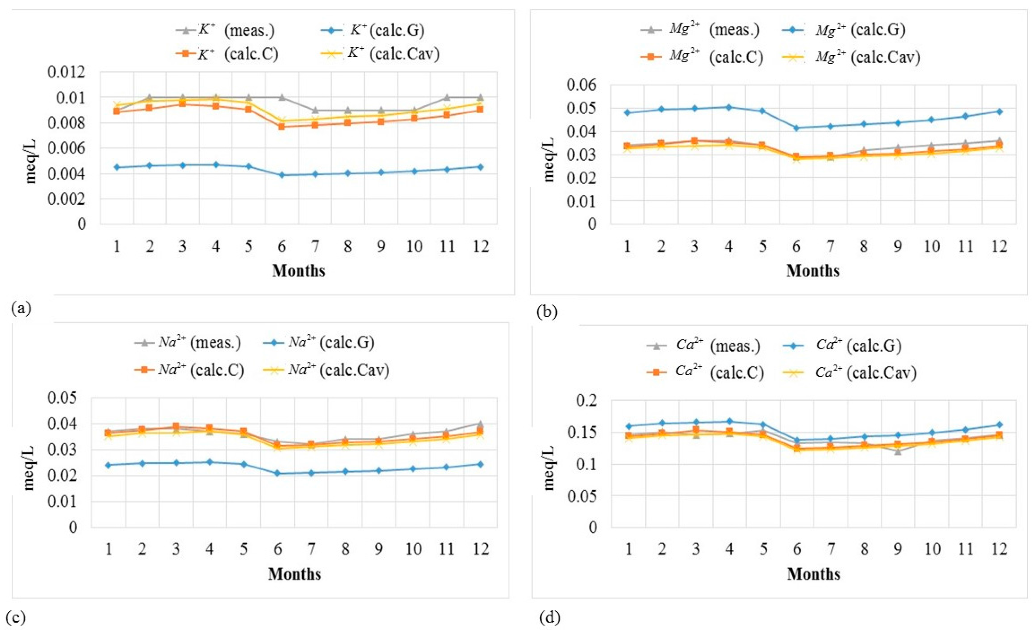
Measured concentrations at four monitoring stations in Swedish rivers were used to test the model for a period of twelve months in order to capture the annual variations. Both model options were used, i.e., the generalized method, which uses the continental averages of relative concentrations (in this case Europe), denoted by (G); and the customized method, which uses the river specific relative concentrations, denoted by (C) and (Cav). The two estimates performed using the customized method differ with regard to the data used to calibrate the model. The estimates denoted by (C) were made using relative concentrations calculated from a single sample during the first month, called the “base month”, to calibrate the model. The estimates denoted by (Cav) were obtained using averages for a period of one year to calibrate the model.
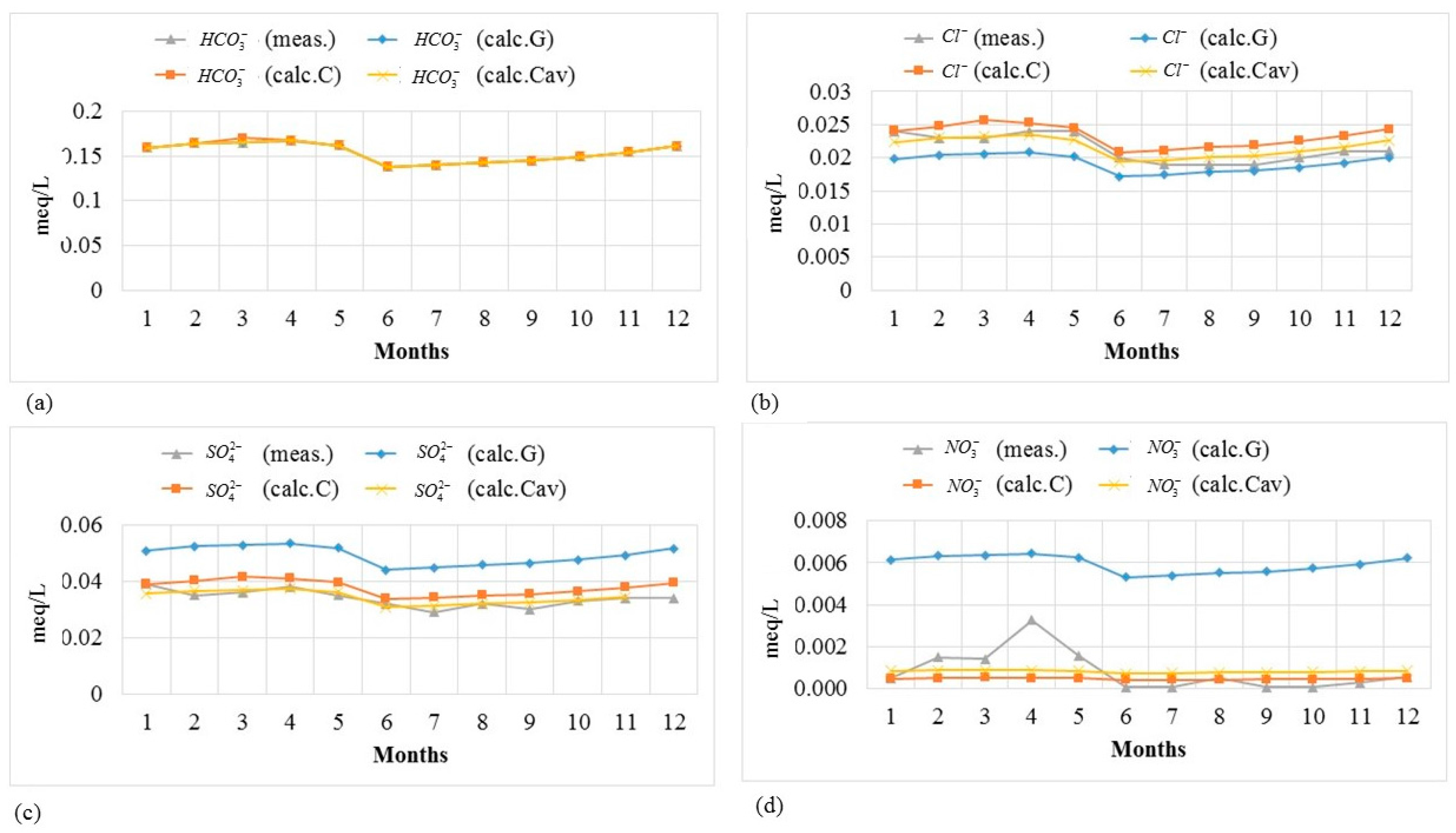
Figure 4 and
Figure 5 show the measured and modeled concentrations of ions for a period of one year at Slagnäs Station in Skellefte älv to illustrate how well the model captures the seasonal variation. The results show that the concentration values estimated by the model are quite similar to the measurements. Equally good results were found for the other three monitoring stations.
Figure 4 and
Figure 5, together with the results of the
RMSE analysis shown in
Table 7, demonstrate that the customized method gives better results than the generalized method, as expected. The model works better to estimate the concentrations of ions with relatively higher concentrations. For nitrate, which, in general, has lower concentrations at all four monitoring stations compared to the other ions, the modelled concentration values are quite different from the measured values; see
Figure 5d.
The values of
RMSE (%) for the
customized method are between 0 and 67%, but about 80% of the
RMSE (%) values are below 15%, for the four stations used in the model validation. For the
generalized method, the corresponding
RMSE (%) values are between 0 and 101% and about 80% of the
RMSE (%) values are below 50%. The analysis of
RMSE (%) was carried out excluding nitrate because its estimates exhibit larger errors and should not be trusted, as stated before, see
Table 7. Sometimes it is possible to obtain better results for some ions using the
generalized method, but this is probably coincidental.
The large errors in the estimated nitrate occur when the nitrate concentrations are being governed by factors other than pH, alkalinity and temperature. These factors include, for example, the increasing concentration of nitrogen in rivers in later autumn, reaching its peak in spring, which is explained by the increasing losses from soils and low biological activity in rivers [
23]. The lower concentrations of nitrogen in the summer and earlier autumn are caused by the consumption by phytoplankton, nitrogen uptake by crops and other biota, and the denitrification processes in soil and groundwater [
23].
In general, there is a small improvement in the estimated values when using the customized method with Cav (employing annual averages of relative concentrations to calibrate the model) compared to the customized method with C (employing a single sample during a base month to calibrate the model). This small improvement is reasonable since the annual averages used to calibrate the model take into consideration the variability of the concentration of each ion due to seasonal changes.
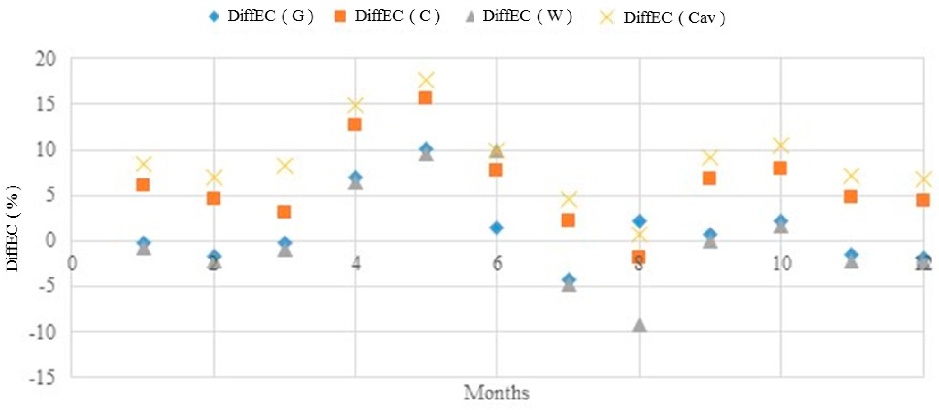
The
DiffEC(%) was also calculated when estimating the concentrations of ions at the four stations used to validate the model, see Equation (13). As an example,
Figure 6 shows
DiffEC(%) for Slagnäs Station in Skellefte älv. The
DiffEC(G) is the difference when using continental averages, in this specific case Europe;
DiffEC(C) and
DiffEC(Cav) are the differences when using the customized method; and the
DiffEC(W) is the difference when using the world averages. Note that there are no estimates of ion concentrations made using the (W) method. The
DiffEC(W) was calculated just to check its variability and to compare with the values obtained by the other methods.
The values of DiffEC(%) for the general method varied between −15% and +40%, but for the customized method it did not go beyond ±20% in relation to the baseline value at all four stations used to validate the model. Therefore, it is recommended that when doing estimates using the general method, the values of DiffEC(%) should be between −15% to +40% and when using the customized method, it is recommended that the values of DiffEC(%) do not go beyond ±20% from the baseline value. Employing the suggested limits on DiffEC(%) there is an 80% probability of having an RMSE (%) below 15% using the customized method and below 50% using the generalized method. If the value of DiffEC(%) goes beyond the suggested limits, the first option is to gather data from the river of interest to recalibrate the model; such deviations might be caused by disturbances to the river system from pollution discharge due to mining or other activities. If the value of DiffEC(%) still remains out of the normal range, the model is not recommended for the specific river; the reason could be that significant amounts of ions, other than the MI considered in the present model, cause considerable variability in the relative concentrations of ions.
The estimates of the concentrations of MI by the model can always be improved by extending the ions considered, thus reducing the DiffEC(%) for the base month. For the generalized method, improvements can be made through better continental averages used by the model (that is, more data) or by reducing the area to become more specific rather than employing continental averages.
In the case of mining, the concentrations of MI are not the only parameters of interest. It is also important to estimate the concentrations of other ions, such as
Fe3+,
Mn4+, and heavy metals. At this stage only
Fe3+,
Mn2+,
Cd2+,
Cu2+,
Al3+,
Pb2+, and
Zn2+ were considered as a demonstration of the potential of the model. The values that can be estimated by the model are the maximum possible concentrations, because it uses the equilibrium approach. The procedure of estimating the concentrations of ions using equilibrium concentrations is well known, see reference [
9], and it is not discussed in detail here. However, a brief discussion follows, about the limitations of employing equilibrium theory to estimate concentrations of ions in natural waters.
The ions in natural waters are usually not in equilibrium with the minerals at the bottom of the stream; thus, the procedure will most likely overestimate the concentrations, which is why the values are considered as maximum possible concentrations. However, it is possible to obtain higher concentrations when measuring non-filtered samples by instrumental methods. This is because the equilibrium theory only estimates the concentrations of free ions. There are some minor ions or heavy metals that tend to appear in water in other forms than free ions. This is the case for iron (Fe) and aluminum (Al), normally used as coagulants in water treatment processes. These elements can easily appear in the form of complexes or be bound to organic matter, and therefore the concentrations estimated by the model using equilibrium equations can be lower than the measured concentrations by instrumental methods. However, estimates by the model are still useful, since the reactivity of elements in water is more related to free ions.
Another potential model improvement, besides expanding the number of ions considered as MI, would be to develop a method to estimate the actual concentrations of minor ions and heavy metals, not the maximum possible concentration.
4. Applicability of the Model and Its Limitations
The proposed model can be used as a simple tool to estimate the concentrations of major ions (Na+, K+, Mg2+, Ca2+, HCO3−, SO42−, Cl−, and NO3− ) as well as some minor ions and heavy metals (Fe2+, Mn2+, Cd2+, Cu2+, Al3+, Pd2+ and Zn2+) in rivers when the pH, alkalinity, temperature, and electric conductivity are known. The model is not recommended for saline water, such as sea water or saline lagoons where the concentrations of ions are very high and the interaction between them is marked, making the ionic strength high.
The model was developed to minimize the input data required and it can be used with limited resources, while still yielding satisfactory estimates. This will make the model suitable for use in developing countries, but also in developed countries when there is no need to have very accurate information about the water quality obtained through sophisticated and costly monitoring programs.
It was difficult to find data good enough to test the model from developing countries. Only data from stations in Swedish rivers was used to test the model. However, it is not a problem, since for any application, the model has to be calibrated using local data. For the generalized method, continental averages are used and for the customized method, baseline data from the specific river to be modelled are used.
As discussed before, when using the generalized method, the model employs continental averages to estimate the relative concentrations of major ions, which may induce large uncertainty. However, this uncertainty can be partly overcome by using the customized method, which, instead of using continental averages, relies on baseline data for the specific river. Even with the uncertainty introduced by the continental averages, the concentrations of major ions estimated using the generalized method are reasonably good, as previously shown, although it is important to consider the recommended limits for DiffEC(%). Unfortunately, it was not possible to validate the predictive capability of the model for several continents or countries, especially for developing countries where the model is expected to be used, due to lack of data. This is something to be investigated in the future; however, the model was tested using Swedish data and gave good results.
There are many possibilities to further develop the model, such as including more ions, finding different methods to estimate the minor ions and heavy metals that do not use equilibrium concentrations, and including complex compounds in the model estimates. All these improvements, however, require data and more detailed studies.
5. Conclusions
A model was developed that uses only pH, alkalinity, and temperature to estimate the concentrations of major ions (MI) in rivers (Na+, K+, Mg2+, Ca2+, HCO3−, SO42−, Cl−, and NO3−) together with the maximum possible concentrations of minor ions and heavy metals (Fe2+, Mn2+, Cd2+, Cu2+, Al3+, Pd2+ and Zn2+). The model was tested using data from four monitoring stations in Swedish rivers.
In order to achieve good accuracy, it is important that the relative concentrations of MI in the water do not change considerably over time. This assumption was reasonably well confirmed by evaluating the trends using the Man–Kendell test together with linear regression for the four stations in Swedish rivers. Using the Man–Kendell test and a significance level of 0.05 it was found that, in most cases, there is sufficient evidence to conclude that there is no trend. The linear regression showed that the changes in relative concentrations during a period of 10 years did not exceed 10%.
The model developed includes two options to make estimates: the generalized method and the customized method. The generalized method uses continental averages of relative concentrations, whereas the customized method uses river specific baseline data, to perform the calibration. The values estimated by the model were compared to the measured data from the four monitoring stations using root-mean-square error, and the results were good. About 80% of the values of RMSE(%) are below 15% for the customized method and below 50% for the generalized method, for the four stations used to validate the model. The errors associated with the estimated concentration of nitrate (NO3−) are too high, and the results for this ion should not be trusted. The generalized method may be employed to obtain an overall estimate of the concentrations of ions in river water in case there is no baseline data for the calibration of the model.
A parameter DiffEC(%) was introduced to quantify the accuracy of the estimates provided by the model based on the difference between the measured and estimated electric conductivity as a percentage. It is recommended that, for the customized method, this value should not vary more than ±20% in relation to the baseline value, and for the generalized method it should be between −15% and +40%. Keeping the suggested limits on DiffEC(%), there is an 80% probability of having an RMSE (%) below 15% when using the customized method and below 50% when using the generalized method.
Although the uncertainties of the model are difficult to estimate, the new methodology of using the relative concentrations of ions was demonstrated to be useful in estimating the concentration of major ions in rivers. In practical applications, the model can be used to get an approximate estimate of the concentrations of MI when there is a lack of data and/or resources.


 ,
, 


