Modeling of Coupled Water and Heat Transfer in Freezing and Thawing Soils, Inner Mongolia

Abstract

Accurate simulation of soil water and heat transfer is critical to understand surface hydrology under cold conditions. Using an extended freezing code in HYDRUS-1D (freezing module), this study was conducted: (1) to evaluate the freezing module using field data collected in a grazed steppe of Inner Mongolia; and (2) to further simulate grazing effects on frozen soil hydrological processes. The experimental data consisted of soil water and temperature profiles measured during freeze-thaw cycles from 2005 to 2006 in two plots (ungrazed since 1979 (UG79) and winter grazing (WG)). To check the sensitivity of the freezing module, a model without a freezing scheme (normal module) was used for comparison. We found that while the normal module can only simulate soil water and heat transfer under unfrozen conditions, the freezing module can simulate well under both frozen and unfrozen conditions. The freezing module can reasonably compute water phase change and, therefore, substantially improved the simulation of the evolution of liquid water and temperature in frozen soil. It overestimated liquid water content during spring snowmelt and, thus, underestimated surface runoff from underlying frozen soil layers. Furthermore, the weak prediction of soil moisture at the WG site, compared with the UG79 site, might relate to the less than ideal parameterization of soil hydraulic properties. Our results confirmed that the freezing module was able to accurately predict behaviors of soil freezing and thawing, as well as the effects of land management. We suggest that detailed knowledge of the soil-atmosphere processes is needed to improve the surface runoff algorithm in the frozen soil module.

1. Introduction

Coupled water, vapor and heat movement in the vadose zone is a central process in many agricultural, ecological and engineering issues [1]. The need for coupled processes is especially true in cold and arid regions, where the annual freezing and thawing cycle of soil might significantly impact soil physical properties and the associated water and heat balance [2]. Frozen soil normally reduces infiltration capacity significantly due to the blocking effects of ice lenses in soil pores. Consequently, lateral flow and snow melt may release large quantities of water in the spring and early summer and cause substantial surface runoff or ponding water [3,4]. Furthermore, this behavior will increase the risk for soil erosion and nutrient loss. Although the former processes are widely recognized, the simulations of snow hydrology and soil freezing and thawing are rarely performed due to limited data availability to parameterize or validate such models and the lack of suitable models that describe the complex processes during phase changes.

Frozen soils are generally characterized by the coexistence of ice and liquid water. Thus, it is necessary to simulate the freezing and thawing process by specifically considering the phase change of ice and water at variable freezing points. Usually, the two prevalent classes of soil freezing and thawing models, namely hydrodynamic models (e.g., [5,6]) and frost heave models (e.g., [7]), have been used. These models mainly differ in the treatment of ice pressure, which is assumed to remain constant in hydrodynamic models and variable in the frost heave models [8]. As a result, the former offers accurate predictions under unsaturated conditions, but fails to predict frost heave, while the reverse situation occurs when using the latter model. In the unsaturated zone in soil science, it is customary to use the hydrodynamic model.

In recent years, efforts have been made to develop frozen soil parameterizations in land surface schemes for atmospheric models [9,10]. Water and energy balances are generally linked at the soil-atmosphere interface and controlled by climatic conditions and soil properties. A challenge with frozen soil parameterization is the difficulties in approximating the hydraulic conductivity in partially frozen soil. Soil freezing may result in dramatic reductions in infiltration rates [11], mainly due to the blocking effects of frozen water in soil pores [8,12]. However, it is often inaccurately predicted because of limited data to parameterize the related processes. Following Lundin, using an experimental method, Zhao et al. [2] measured the reduced hydraulic conductivity by blocking effects, i.e., defined impedance parameter, which had been incorporated into the freezing module of the HYDRUS model. This inclusion advanced the parameterization of frozen soil hydraulic conductivity in the numerical model.

To simulate water flow in the partly frozen soils, it is essential to know not only how to express the unsaturated hydraulic conductivities of the frozen soils, but also the impacts on the soil water retention curve (SRC; relationship between soil water and pressure head) and the coupled soil freezing curve (SFC; relationship between soil water and sub-zero temperature). Koopmans and Miller [13] measured the SFC and SRC of the same soils under freezing and drying processes and found a unique relationship between the negative temperature at which a given unfrozen water content occurs and the matric potential corresponding to a similar moisture content at room temperature. This relationship was seen as a function of temperature alone by using the generalized Clapeyron equation. Harlan [5] derived the SFC from SRC using this relationship, assuming the same pore geometry for both frozen and unfrozen soils. However, numerical simulations indicated that this assumption overestimated water flow near the freezing front. Currently, Harlan’s concept and the impedance factor have been considered in several numerical codes, e.g., SHAW [6] and HYDRUS [14].

Studies have shown that the models with an explicit frozen soil scheme give a much more realistic soil temperature simulation during the winter than those models without a frozen scheme [15]. A frozen soil model with realistic simulation of soil temperature, moisture content and ice content also improves the climate model’s ability to simulate greenhouse gas exchange processes in cold regions [16]. These findings emphasize the need to better understand snowmelt and freezing and thawing processes. Currently, there are several numerical codes, e.g., SVAT [17], SHAW [6] and HYDRUS [14], developed for simulating coupled water and heat flow in frozen soils. However, these numerical models are limited to the mutual interactions between water and heat flows in the frozen soil in terms of laboratory observation and/or field applications. All of these interactive effects through the coupling of thermal and hydrological processes are more prominent in the frozen zone with abrupt phase transitions. However, only a few schemes for frozen soil deal with these cross effects [18]. In terms of the freezing module in the HYDRUS model, it must be validated by field-measured data according to the short-term laboratory tests by Hansson et al. [8].

A complication in performing the simulations is that soil heat and water regimes may be modified by different land uses, which are further complicated by snow melt and soil freezing and thawing processes. For instance, a platy soil structure may result from animal trampling during grazing in winter and is associated with frost-created platy aggregates [19]. Thus, lateral water movement on the upper frozen layer is expected to be high during soil thawing, as a frozen and platy-structured underlying soil horizon prevents infiltration [3]. For Inner Mongolia grasslands, despite the existence of little winter precipitation, the snowmelt might create annual peak discharge due to an abrupt transition to higher temperatures in spring. During this period, the frozen soil layers impede infiltration and retention of melt water in the deeper soil layers and, consequently, create lateral flow [12]. These changing relationships require a full integration of the interwoven thermo-hydro-mechanical interactions in transport modeling [20].

In Zhao et al. [21], grazing effects on soil hydraulic and thermal properties have been parameterized by calibrating the model HYDURS-1D, based on data for soil moisture and temperature measurements, water interception (obtained by the model SHAW) and hydraulic parameters (laboratory-derived hydraulic properties). This work was limited to show the effects of grazing on coupled water and heat fluxes during the growing period, i.e., unfrozen conditions. Here, we particularly attend to the snowmelt and soil freezing and thawing processes. This study addresses the field application of the hydrodynamic model HYDRUS-1D for frozen soil conditions. In the current newest program, an extended freezing code is incorporated, which numerically solves coupled equations governing phase changes between water and ice and heat transport with a mass- and energy-conservative method [8]. Our objectives are: (1) to assess the model ability in reflecting soil freezing and thawing dynamics using field-measured data in a grazed steppe; and (2) to simulate grazing effects on frozen soil hydrological processes. For those aims, two field plots with different grazing intensities were selected and compared.

2. Materials and Methods

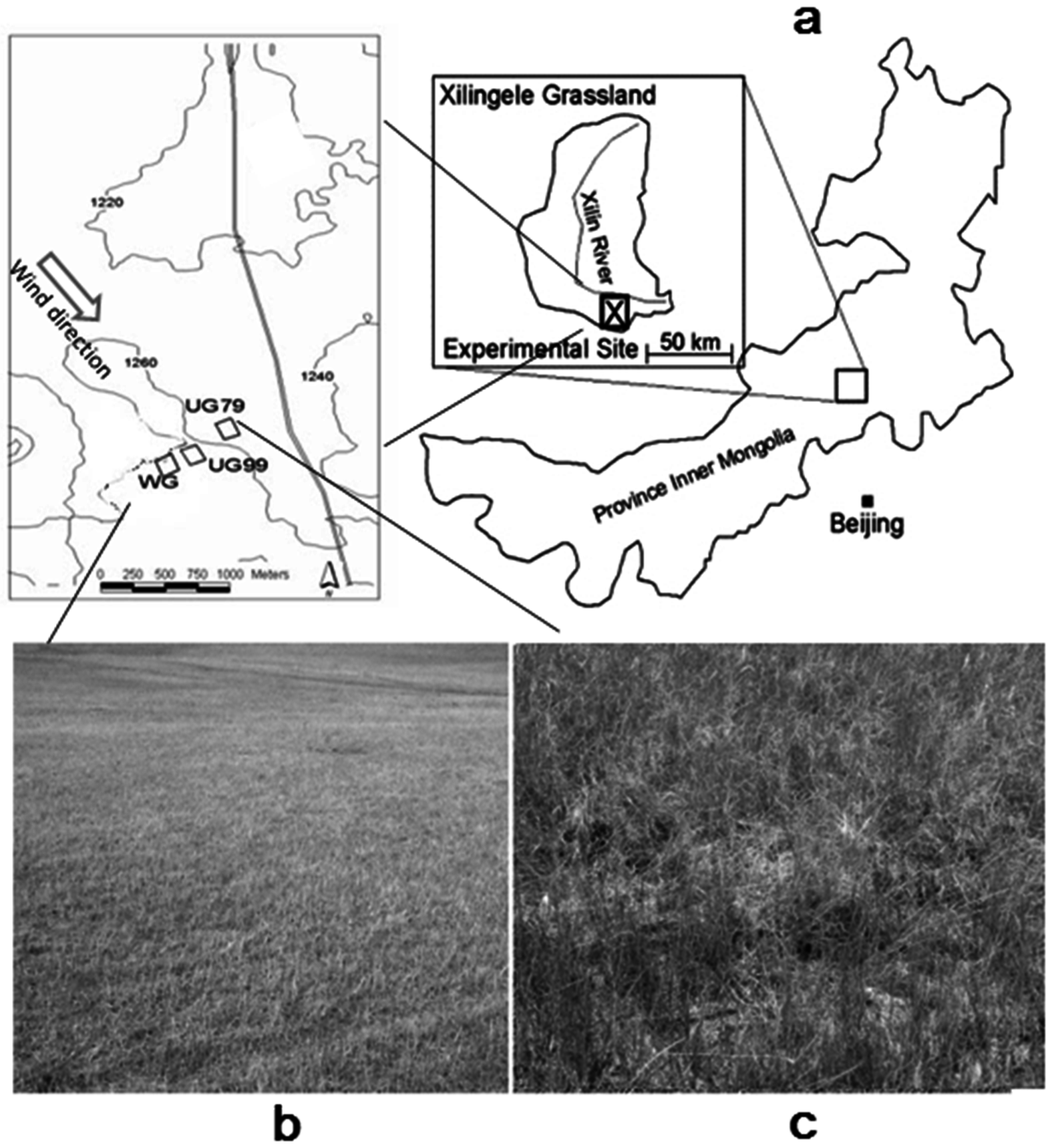
2.1. Study Area

The study was performed at a long-term experimental site of the Inner Mongolia Grassland Ecosystem Research Station (IMGERS, 43°37′50′′ N, 116°42′18′′ E). During the period of 2004–2009, soil moisture and temperature were recorded by a data-logger (DL2e, Delta-T Devices, Cambridge, UK) at 30-min intervals in summer and at 1-h intervals in winter under four different grazing intensities, respectively [22]. Soil water content was measured at 5-, 20- and 40-cm depths by theta-probes (Type ML2x, Delta-T Devices, Cambridge, UK). In cases where the soil is frozen, the theta-pore reading refers to the volumetric unfrozen water content. Soil temperature was measured at soil depths of 2, 8, 20, 40 and 100 cm using platinum ground temperature probes (Pt-100, Omega, Manchester, UK). Precipitation and other weather variables, such as net radiation, air temperature, relative humid, and wind speed were recorded by a standard micrometeorological station (located 50 m from the monitoring plot; Ketzer et al. [23]). Winter precipitation as snow was treated as a snow water equivalent during measurement and calculations when the air temperature was lower than 0 °C [24]. Snow water equivalent was measured using a 50-mm internal diameter aluminum snow-survey tube. To determine root length density, root samples were taken to a 100-cm depth. In addition, undisturbed soil samples were taken at several depths to determine the water retention characteristics and hydraulic conductivities.

Zhao et al. [22] reported that strong annual cyclic characteristics were displayed for soil moisture and temperature during long-term monitoring. In this study, we only focused on a 1-year dataset including complete soil freezing and thawing cycles. For the comparison of grazing impacts, we selected two contrasting sites with identical topography, but that differ in their grazing intensity [25]. One 24-ha site (ungrazed since 1979 (UG79)) was fenced in 1979 and had not been grazed since that time. The other 40-ha site (winter grazing (WG)) had been moderately grazed (2 sheep ha⁻¹) from 1979 to 2001 and was then used for winter grazing, in which grazing had been prevented between May and October, and there were about 4–5 sheep ha⁻¹ grazed from November to April. The soil at both sites is a sandy-loam texture, but with slightly more clay at the WG site (

Table 1. The basic soil parameters at the two investigated sites used in the model. UG79: ungrazed since 1979; WG: moderately grazed.

Treatment	Soil Depth (cm)	Sand (%)	Silt (%)	Clay (%)	Bulk Density (g·cm−3)	Soil Organic Carbon (g·kg−1)	θr (cm3·cm−3)	θs (cm3·cm−3)	α (cm−1)	n (-)	Ks (cm·day−1)
UG79	4–8	62.0	22.2	15.8	1.14	22.0	0.075	0.572	0.026	1.766	165.0
	18–22	73.0	14.6	12.4	1.39	16.5	0.086	0.472	0.019	2.199	133.3
	30–34	78.1	11.0	10.9	1.44	10.1	0.079	0.453	0.015	2.549	113.7
	40–44	78.7	11.6	9.7	1.43	8.2	0.071	0.452	0.016	2.120	71.9
WG	4–8	53.7	27.2	19.1	1.18	22.2	0.075	0.57	0.021	1.636	54.7
	18–22	58.4	23.9	17.7	1.29	13.2	0.050	0.526	0.023	1.616	69.8
	30–34	59.3	24.3	16.5	1.27	11.4	0.072	0.529	0.012	1.791	72.7
	40–44	60.4	22.8	16.9	1.34	11.6	0.079	0.517	0.014	1.742	61.3

), and is classified as a Mollisol according to the USDA [26]. The upper 4 cm are CaCO₃-free, but deeper soil layers contain significant amounts of carbonate [27]. The vegetation is dominated by a perennial rhizome grass, Leymus chinensis and Stipa gradis steppe. Differences were observed with vegetation coverage and dead standing plant material being greater at the UG99 site than at the WG site (Figure 1).

2.2. Liquid and Ice Water Flow

Simulations of soil water, vapor and heat flow were performed with the extended freezing module of the HYDRUS-1D software package [8]. Variably saturated water flow for above- and sub-zero temperatures is described using the modified Richards equation:

$$\frac{\partial {\theta }_u(h)}{\partial t}+\frac{p_i}{p_w}\frac{\partial {\theta }_i(T)}{\partial t}=\frac{\partial }{\partial z}\left[K_{Lh}\frac{\partial h}{\partial z}+K_{Lh}+K_{LT}\frac{\partial T}{\partial z}+K_{vh}\frac{\partial h}{\partial z}+K_{vT}\frac{\partial T}{\partial z}\right]-S$$

(1)

where θ_u (L³·L⁻³) is the volumetric unfrozen water content (= θ + θ_v; θ and θ_v are the volumetric liquid and vapor water content, respectively); θ_i is the volumetric ice content; p_w and p_i are the density of liquid and ice water, respectively; t is the time; z is the soil depth; h is the pressure head; T is the temperature; and S is a sink or source term, which normally accounted for root water uptake. In Equation (1), the first five terms on the right-hand side represent liquid flows due to gradients in the pressure head (K_Lh, (L·T⁻¹)), gravity and temperature (K_LT, (L² T⁻¹·K⁻¹)) and vapor flows due to gradients in the pressure head (K_vh) and temperature (K_vT), respectively.

Equation (1) is highly nonlinear, because of the dependencies of the water content and the hydraulic conductivity on the gradients of pressure head and temperature, i.e., θ(h), θ_i(T), K_Lh(h) and K_LT(h). The K_Lh is described by the following expressions [29]:

$$S_e(h)=\frac{\theta (h)-{\theta }_r}{{\theta }_s-{\theta }_r}=\frac{1}{{(1+{\left|\alpha h\right|}^n)}^m}$$

(2)

$$k_{Lh}(h)=k_s\times S_e^l{(1-{(1-S_e^{1/m})}^m)}^2$$

(3)

where S_e is the effective saturation; θ_s and θ_r are the saturated and residual water contents, respectively; the symbols α (L⁻¹), n and m = 1 − 1/n are empirical shape parameters; and the inverse of α is often referred to as the air entry value or bubbling pressure; K_s is the saturated hydraulic conductivity (L·T⁻¹); and l is a pore connectivity parameter.

The hydraulic conductivity of frozen soil is significantly reduced by ice lens, which is accounted for by an impedance factor, Ω [30]:

$$K_{fLh}{=10}^{-\mathsf{\Omega }\mathrm{Q}}{K}_{Lh}$$

(4)

where the parameter Q is the ratio of the ice content to the total water content (i.e., θ_i/(θ_i + θ_u)), which accounts for the more significant blocking effects with the increase in ice content. The impedance parameter is set as 4.2 based on our measurement [2].

The thermal hydraulic conductivity, K_LT, is defined as follows (e.g., [31]):

$$K_{LT}=K_{Lh}(h{G}_{wT}\frac{1}{{\gamma }_0}\frac{d\gamma }{dT})$$

(5)

where G_wT is the gain factor, which quantifies the temperature dependence of the soil water retention curve [32], γ is the surface tension of soil water (= 75.6 − 0.1425T − 2.38 × 10⁻⁴ T² g·s⁻²) and γ₀ is the surface tension at 25 °C (= 71.89 g·s⁻²).

2.3. Soil Heat Transport

The governing equation for the movement of energy in a variably-saturated rigid porous medium is given by the following conduction–convection heat flow equation (e.g., [8]):

$$\frac{\partial C_{p}T}{\partial t}-L_f\rho i\frac{\partial {\theta }_i}{\partial t}+L_0(T)\frac{\partial \theta v(T)}{\partial t}=\frac{\partial }{\partial z}\left[\lambda (\theta )\frac{\partial T}{\partial z}\right]-C_w\frac{\partial q_{l}T}{\partial z}-C_v\frac{\partial qvT}{\partial z}+L_0(T)\frac{\partial qv}{\partial z}-C_{w}ST$$

(6)

where L_f is the latent heat of freezing and L₀ is the volumetric latent heat of water vaporization, respectively. In Equation (6), the three terms on the left-hand side represent changes in the energy content, the latent heat of the frozen and vapor phases, respectively. The terms on the right-hand side represent, respectively, soil heat flow by conduction, convection of sensible heat with flowing water, transfer of sensible heat by the diffusion of water vapor, transfer of latent heat by the diffusion of water vapor and the uptake or provision of energy associated with the sink or source term. C_p is the volumetric heat capacity of the bulk soil, which is determined as the sum of the volumetric heat capacities, including solid (C_n), organic (C_o), liquid (C_w), ice (C_i) and vapor (C_v) phases multiplied by their respective volumetric fractions [33].

The symbol λ(θ) in Equation (6) denotes the apparent thermal conductivity; q is the water flux density, and T is the soil temperature. The apparent thermal conductivity combines the thermal conductivity of the porous medium in the absence of flow and the macro-dispersivity, which is assumed to be a linear function of velocity and modified as follows:

$$\lambda (\theta )={\lambda }_0(\theta )+\beta C_w\left|q_L\right|$$

(7)

$${\lambda }_0(\theta )=b_1+b_2({\theta }_w+F{\theta }_i)+b_3{({\theta }_w+F{\theta }_i)}^{0.5}$$

(8)

where β is the thermal dispersivity (m). The thermal conductivity, λ₀(θ), is described with a simple equation given by [34]. The ice enhancement factor F (–), compensating for the higher thermal conductivity of ice with respect to water, was defined by [8] as follows:

$$F=1+F_1{{\theta }_i}^{F_2}$$

(9)

where F₁ and F₂ are empirical parameters.

The phase change between water and ice is controlled by the generalized Clapeyron equation, which defines a relationship between the liquid pressure head and temperature when ice is present in the porous material [35]. Hence, the unfrozen water content can be derived from the liquid pressure head as a function of temperature alone when ice and pure water co-exist in the soil. The form of the generalized Clapeyron equation was:

$$h=\frac{L_f}{g}\ln \frac{T}{T_0}$$

(10)

where g is the gravitational acceleration (L·T⁻²), T is the temperature (K) and T₀ = 273.15 K is the freezing point of free water.

2.4. Initial and Boundary Conditions

In this study, value-specified initial and boundary conditions at each site were used. Initial conditions were set in the model in terms of measured moisture and temperatures at the beginning of the simulation period. An atmospheric boundary condition, including solving surface energy balance and a free drainage condition, was imposed at the soil surface and bottom boundary of the flow domain, respectively [1]. The potential evapotranspiration was estimated from the FAO Penman–Monteith equation [36]. The potential evaporation and transpiration was partitioned according to Beer’s law as a function of cover area index of material covering the soil (see details in Zhao et al. [21]). The soil profile was considered to be 100 cm deep. Root water uptake was simulated using the model of Feddes et al. [37].

2.5. Water and Heat Flow Simulations

In this study, the current HYDRUS-1D version including the soil frozen code (denoted as the freezing module) was employed to consider the phase changes between water and ice, as well as the surface energy and water balances. The total variably saturated water flow and heat transport equations (Equations (1) and (6)) were both solved numerically using the finite element method for spatial discretization and finite differences for the temporal discretization. The freezing module either can consider continuous values of the net radiation and other meteorological variables measured at any time interval, which are then used directly in the energy balance equation, or can calculate the continuous values from daily meteorological data. The algorithms in HYDRUS-1D for the description of soil temperature and water movement during the freezing and thawing process were tested and adjusted to the local conditions. To verify the function of the freezing module, the “normal” version, including the snow hydrology component without the soil frozen code (denoted as the normal module), was also run as a reference. In the algorithm of snow hydrology, it was assumed that all precipitation is in the form of snow when the air temperature (soil surface) is below −2 °C and in the form of liquid when the air temperature is above 2 °C. There is a linear interpolation between −2 and 2 °C, i.e., 50% of precipitation is snow and 50% is water for a temperature equal to zero [38]. The soil profile was considered to be 100 cm deep, with observation nodes located at 0-, 5-, 20-, 40- and 100-cm soil depths. Three soil layers were defined according to the measured and calibrated layered-soil parameters [21].

Grazing-induced changes in soil physical parameters were also considered in our simulation. In Zhao et al. [21], soil hydraulic and thermal parameters were proven to be a function of grazing intensity under unfrozen conditions. For instance, the van Genuchten hydraulic parameters θs, α and Ks are smaller and θr and n are larger at the grazed sites than those at the ungrazed sites due to the grazing-induced soil compaction. Under freezing conditions, the differences in those parameters might be enlarged due to the blocking effects of ice lenses. Furthermore, Zhao et al. [39] showed that the thermal parameters were also influenced by the grazing intensity. Soil heat capacity decreases with increasing grazing intensity due to higher water contents at the ungrazed sites and similar soil textural classes for each site (Equations (7)–(10)). Thermal conductivity, which shows a non-linear dependency on water content and geometrical arrangement of particles, has also been included in the current freezing module (e.g., Equation (9)). Model accuracy is evaluated in terms of root mean square error (RMSE) [40], which is defined as:

$$RMSE=\sqrt{\frac{1}{N}{\displaystyle \sum _{i=1}^N{(P_i-O_i)}^2}}$$

(11)

where N is the number of observations and P_i and O_i are the simulated and measured values, respectively.

3. Results and Discussion

3.1. Grazing Effects on Soil Properties, Soil Water and Temperature Regimes

Sand content and bulk density were greater and soil organic carbon was less in the subsoil (18–44 cm) than the topsoil layer (4–8 cm) for both sites (Table 1). Site UG79 had greater sand content in the topsoil than the WG site and is related to its sandy parent material. The bulk density of the topsoil significantly increased with increasing grazing intensity (p < 0.05), due to animal trampling. Below the topsoil layer, soil physical properties were not significantly influenced by hoof compaction [21]. Water retention characteristics, represented by van Genuchten parameters, also reflected the differences in pore size distribution at the different sites. Saturated hydraulic conductivities (Ks) decreased with increasing soil depth at the UG79 site, but not for the WG site where Ks showed no depth-dependent trend. An increase of Ks was observed in the WG site compared to the UG79 site, which may be attributed to improved pore continuity resulting from over twenty years without grazing.

Table 2. Monthly-averaged soil temperatures in different depths at the two investigated sites from October 2005 to September 2006. UG79: ungrazed since 1979; WG: moderately grazed in winter.

Treatment	Depth (cm)	Month (October 2005–September 2006)												Average in Winter	Period of Ground Freezing (Day)
		10	11	12	1	2	3	4	5	6	7	8	9
UG79	2	5.1	−5.3	−12.9	−13.6	−11.5	−4.3	4.2	15.5	18.5	20.8	22.2	11.0	−7.2	144
	8	5.7	−4.3	−11.8	−12.9	−11.2	−4.6	3.5	13.8	17.6	20.2	21.3	11.6	−6.9	146
	20	6.7	−2.5	−9.8	−11.5	−10.3	−4.9	2.4	11.2	16.1	19.0	20.1	12.4	−6.1	145
	40	8.0	−0.1	−6.9	−9.4	−8.9	−5.0	0.9	8.4	13.9	17.1	18.5	13.3	−4.9	148
	100	10.2	4.6	−1.0	−4.2	−5.2	−4.0	−0.9	4.3	9.4	13.1	14.9	13.7	−1.8	136
WG	2	4.9	−5.5	−14.8	−15.5	−12.6	−4.5	4.7	15.9	19.0	21.1	22.6	12.2	−8.0	143
	8	4.9	−5.2	−14.3	−15.3	−12.8	−5.2	3.8	14.0	17.8	20.4	21.6	12.0	−8.2	146
	20	6.8	−2.5	−11.1	−13.2	−11.4	−5.3	2.5	10.9	15.9	19.0	20.2	12.8	−6.8	145
	40	7.2	−1.6	−9.6	−12.1	−10.7	−5.3	2.1	9.9	15	18.3	19.6	12.9	−6.2	144
	100	9.8	4.7	−1.0	−4.7	−5.5	−3.8	−0.8	3.4	8.1	12.0	13.9	12.6	−1.9	136

shows soil temperatures during the studied periods as a function of soil depth at the two sites. At the WG site, the topsoil (2 cm) began to freeze on 6 November 2005, i.e., the date from which the daily mean temperature became successively negative. As expected, with increasing soil depth, the freezing process started progressively later. The soil at the 100 cm depth did not freeze until 12 December 2006. Furthermore, the thawing process shows a similar trend with depth; the deeper soil layers begin to thaw later. The duration of ground freezing is consistently 140–150 days within the 100-cm depth and is substantially reduced with increasing soil depth.

The highest monthly average soil temperature in the study period occurs for the surface soil in August for both sites and is 22.2 °C for site UG79 and 22.6 °C for site WG (Table 1). Though the UG79 site had higher monthly average temperatures than the WG site, the difference between the two sites is less than 1 °C. The lowest monthly average temperature occurred in January and is −13.6 °C for site UG79 and −15.5 °C for site WG. In contrast to the summer temperatures, site UG79 had higher temperatures in the winter, and the differences in temperatures between the two sites are much larger and can be as high as 2.7 °C at the soil depth of 40 cm. Soil temperature is obviously affected by grazing intensity, and the monthly mean of soil temperature decreases in winter and increases in summer with increasing grazing intensity. These differences are attributed to the differences in thermal insulation at the soil surface. The dense vegetation at the ungrazed sites (Figure 1) protects soil from receiving strong radiation in summer, resulting in lower soil temperatures in the summer. In the winter, however, the litter/residue coverage reduces energy loss from the soil to the atmosphere because of the lower thermal conductivities in the winter. It was also observed that the soil temperature amplitudes are higher for the grazed sites than the ungrazed sites.

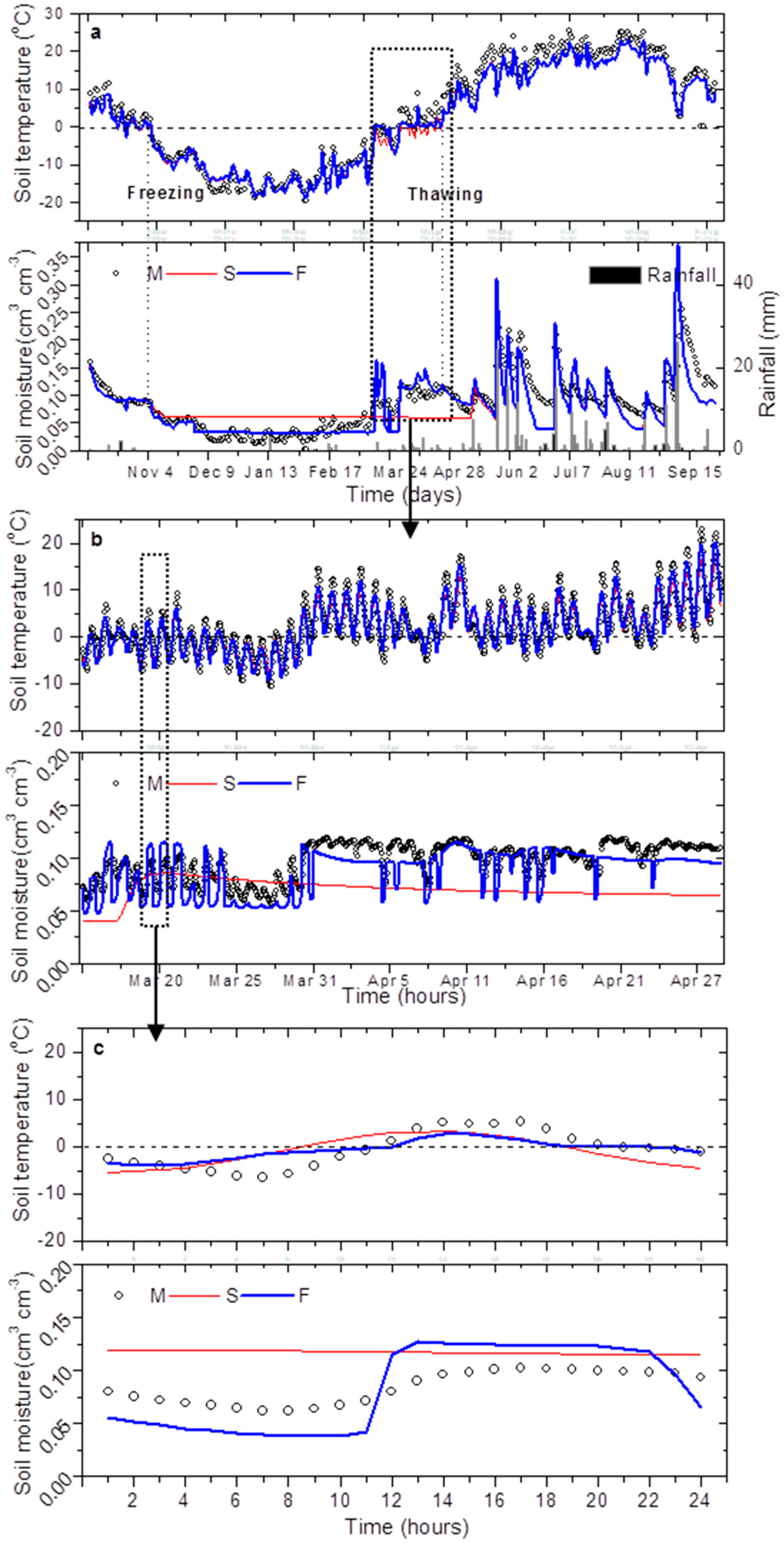
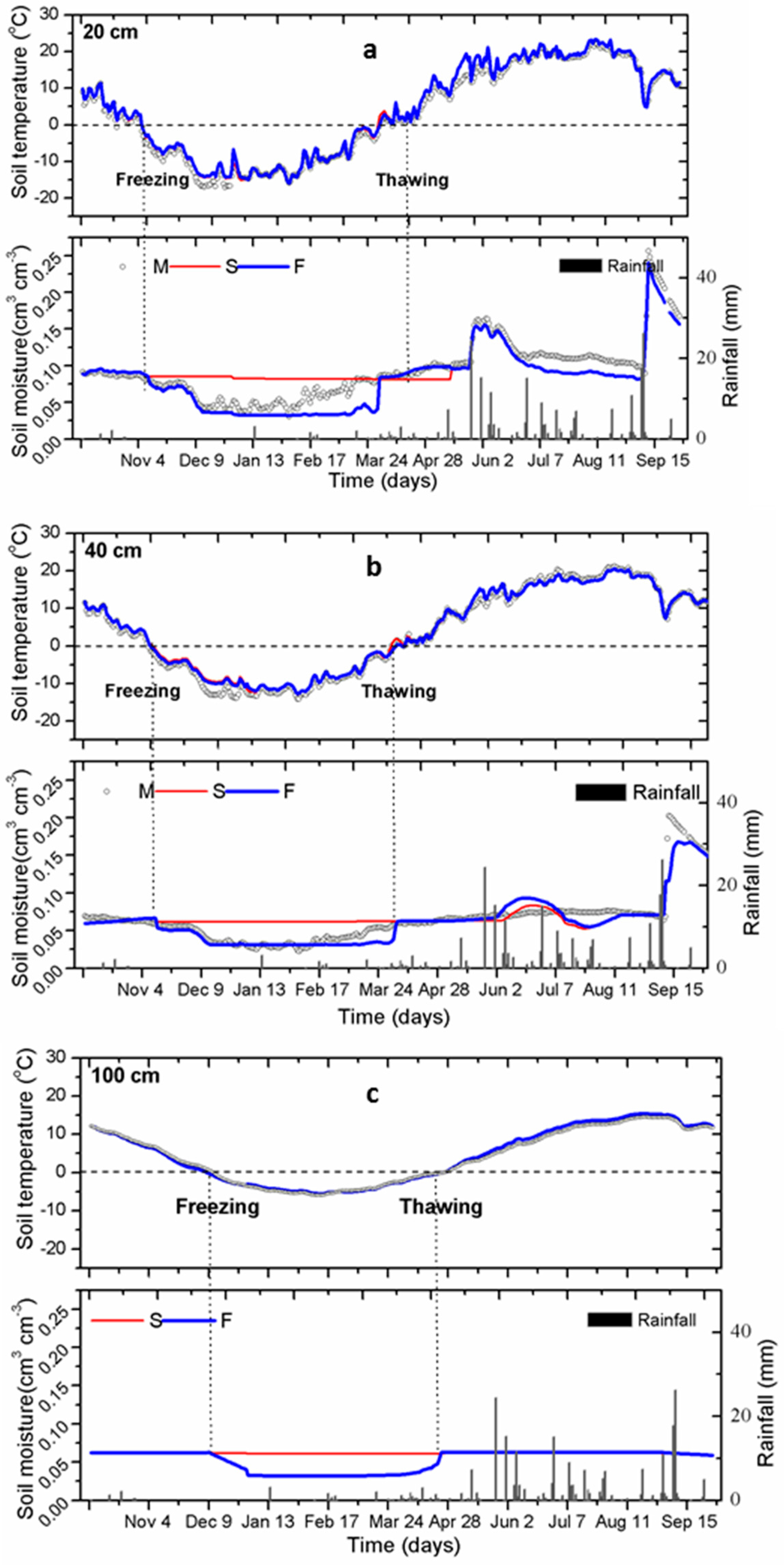
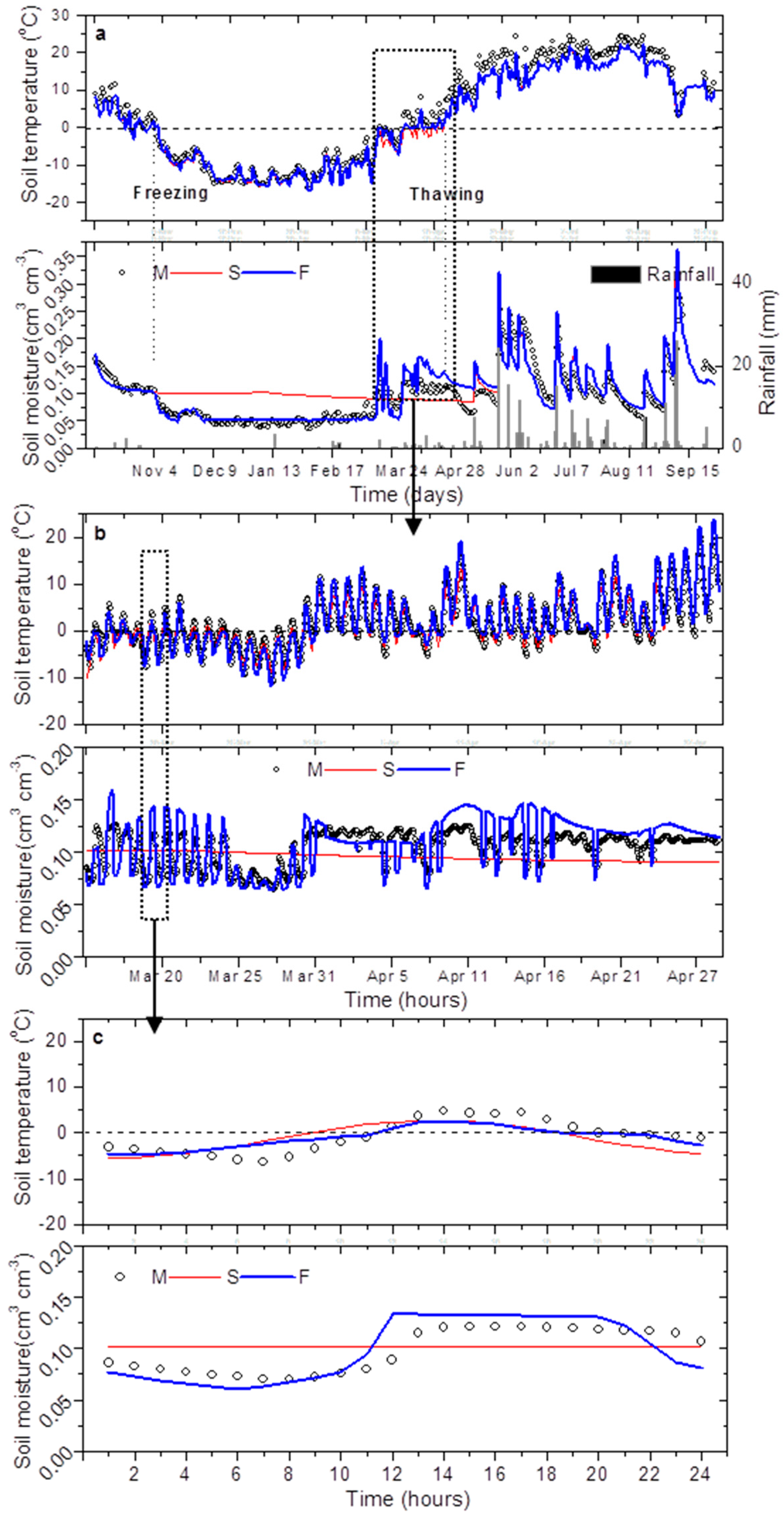
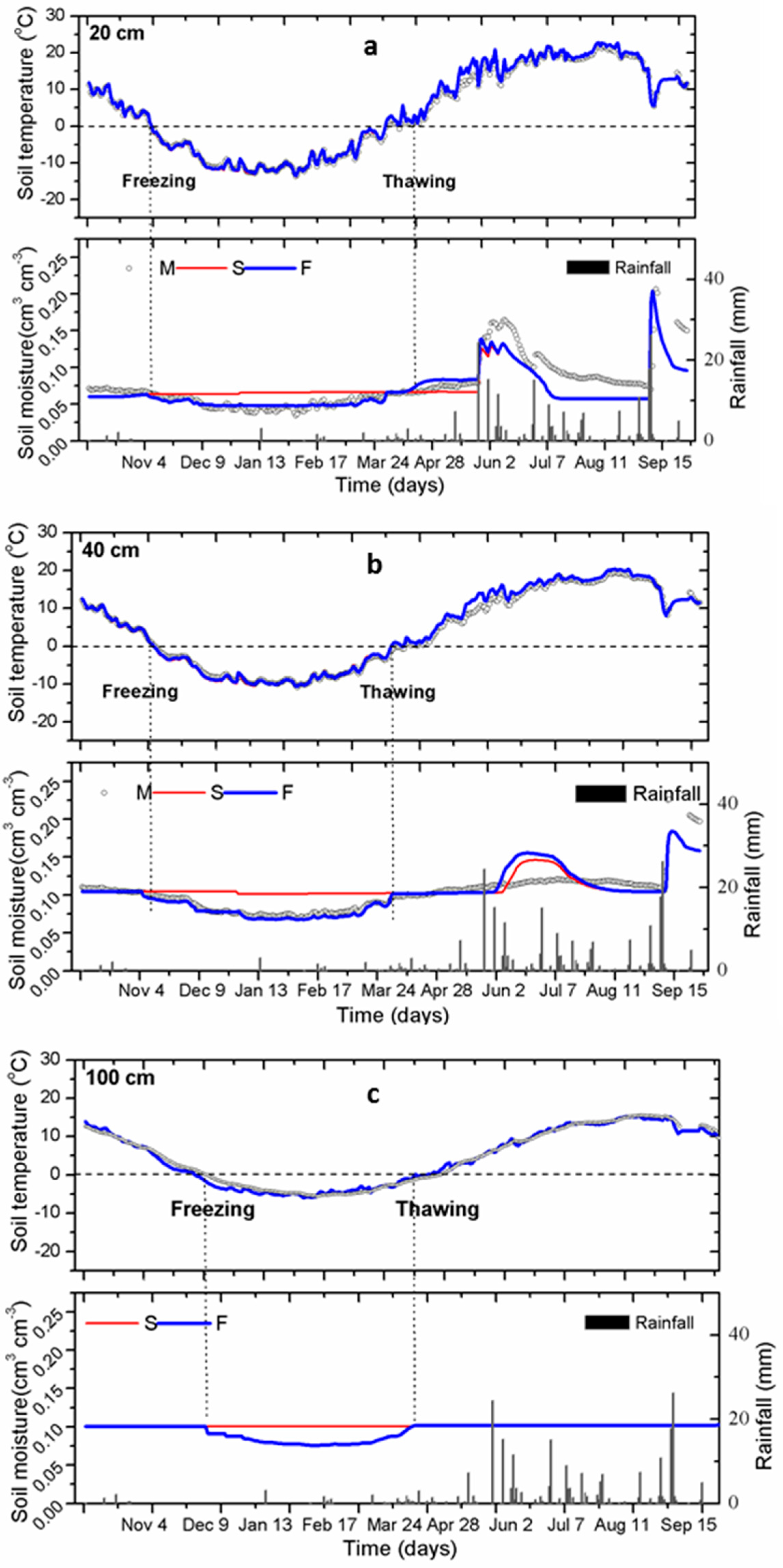
3.2. Simulated Soil Temperatures and Water Contents

Soil water and heat fluxes were numerically simulated for 2006 at site UG79 (Figure 2 and Figure 3) and site WG (Figure 4 and Figure 5). The simulated and measured soil water contents (SWC) are generally comparable during the studied period in terms of root mean square errors (0.02–0.07 cm³·cm⁻³ for UG79 and 0.02–0.08 cm³·cm⁻³ for WG). There is good agreement between the measured and simulated responses to rainfall amounts at the 5-cm soil depth for the WG site (Figure 2a). Soil moisture increased sharply right after each significant rainfall event for the WG site. However, soil moisture at the 5-cm depth at the UG79 site responded only to two large rainfall events and had little response to other rainfall events. The different soil moisture response to the rainfall events between the two sites is primarily attributed to the differences in vegetation cover. As shown in Figure 1, the UG79 site had much thicker vegetation cover than the WG site. The thicker vegetation covers at the UG79 site resulted in substantial rainfall interception, which easily was evaporated, preventing most rainfall events from infiltration to the 5-cm depth and beyond.

The freezing module provides good estimations of the diurnal water dynamics, which coincides with soil freezing and thawing cycles, i.e., soil moisture increases with increasing soil temperature and vice versa (Figure 2b and Figure 4b). These results suggest that the freezing and thawing processes can be very accurately simulated by the applied freezing code. These results are somewhat better than our expectations, since in the literature, there are few works simulating soil freezing and thawing behavior in such an accurate and detailed fashion. Note that although the initial freezing code in HYDRUS was previously described [8], it has not yet been validated by actual field-measured observations. In contrast, the normal module only fits SWC under unfrozen conditions. Under frozen conditions, there are clear disparities between the liquid water content line simulated by the freezing module and the total water content line simulated by the normal module (Figure 2a). Note that the new equations currently implemented in the freezing module only work under frozen soil conditions. Otherwise, the two modules (i.e., freezing code and normal code) are the same. Therefore, this discrepancy is apparently related to differences in computing soil water transfer and the solution of Richards’ equation between the two modules and may be used to approximate the ice content in the soil considering that the total water contents between two simulations are comparable. From this perspective, the comparison between the two models just provides a way to calculate the ice content, given that there has been no strong water migration during soil freezing and thawing processes [41]. For instance, the SWC simulated by the freezing module drops shortly after 6 November 2005 associated with the soil freezing at site UG79 (Figure 2a). However, the SWC simulated by the normal module remains constant. From these differences, an ice content of 0.07 cm³·cm⁻³ may be estimated. Similarly, the ice content at site WG is 0.05 cm³·cm⁻³ (Figure 4a). It should be mentioned that currently, it is difficult to accurately and precisely measure soil ice water content in the field based on either thermo-time domain (TDR) techniques [42] or the heat pulse method [43]. Recently, Tian et al. [44] used a thermo-time domain reflectometry (T-TDR) probe to determine soil ice content during freezing and thawing and found that T-TDR probes were able to measure soil ice content changes with acceptable accuracy at temperatures below −5 °C, but failed at temperatures between −5 and 0 °C because of temperature field disturbances from the latent heat of fusion. Alternative methods, such as a combination of neutron probe and dielectric permittivity measurements, require different sampling locations so that the sensors do not interfere with each other [41].

When soil temperature increased to above 0 °C in late March, both measured and simulated SWC by the freezing module increased at the 5-cm soil depth, while simulated SWC by the normal module remained constant (Figure 3 and Figure 5). This difference further indicates that the freezing module provides good estimations of increases in the SWC due to soil thawing. An increase in the SWC in the subsoil layers (20 and 40 cm) accompanied by soil thawing was also clearly predicted (Figure 3 and Figure 5). However, there were no indications of vertical water movement since the soil water content is relatively low in comparison to the maximum values of soil water retention. Note that the discrepancies of measured and simulated water might stem from the model representation of the physical processes involved in the freezing of unsaturated soil. For instance, the current HYDRUS freezing module, like other similar models, assumed that the phase transition between ice and liquid water reaches equilibrium instantaneously, even though we know the process likely is not instantaneous.

In contrast to the soil water simulations, the soil temperature is simulated reasonably well by both the freezing module and normal module (Figure 2, Figure 3, Figure 4 and Figure 5). It should be noted that the freezing module matches the detailed diurnal variations of measured soil temperatures better than the normal module under frozen soil conditions (Figure 2c and Figure 4c). These differences provide evidence of the impact of the function of the frozen soil module on soil temperature simulations, as an indication of the model credibility to solve the coupled equations governing liquid water, freezing water and heat transport and making a temperature prediction using the coupled equations. Water that penetrates into a partially frozen soil serves as a potential source of latent heat, although initially, it may simply increase the liquid water content and the temperature of the frozen soil layer [4]. When the soil freezes, soil temperature decreases, and energy is released, which is subsequently used to warm up the soil. However, given that no changes occur in the soil water content, the thermal conductivity of frozen soil would be higher than that of the unfrozen soil due to the presence of ice. Consequently, the upward soil heat flux would be higher when the soil gets frozen, and thus, it tends to make the soil cooler [45]. However, the effect of thermal conductivity is likely to be much smaller than that of the water phase change. Consequently, the freezing module, which considers both processes, provides a more reasonably and realistic simulation of soil temperature and, thus, the duration of freezing than the normal module.

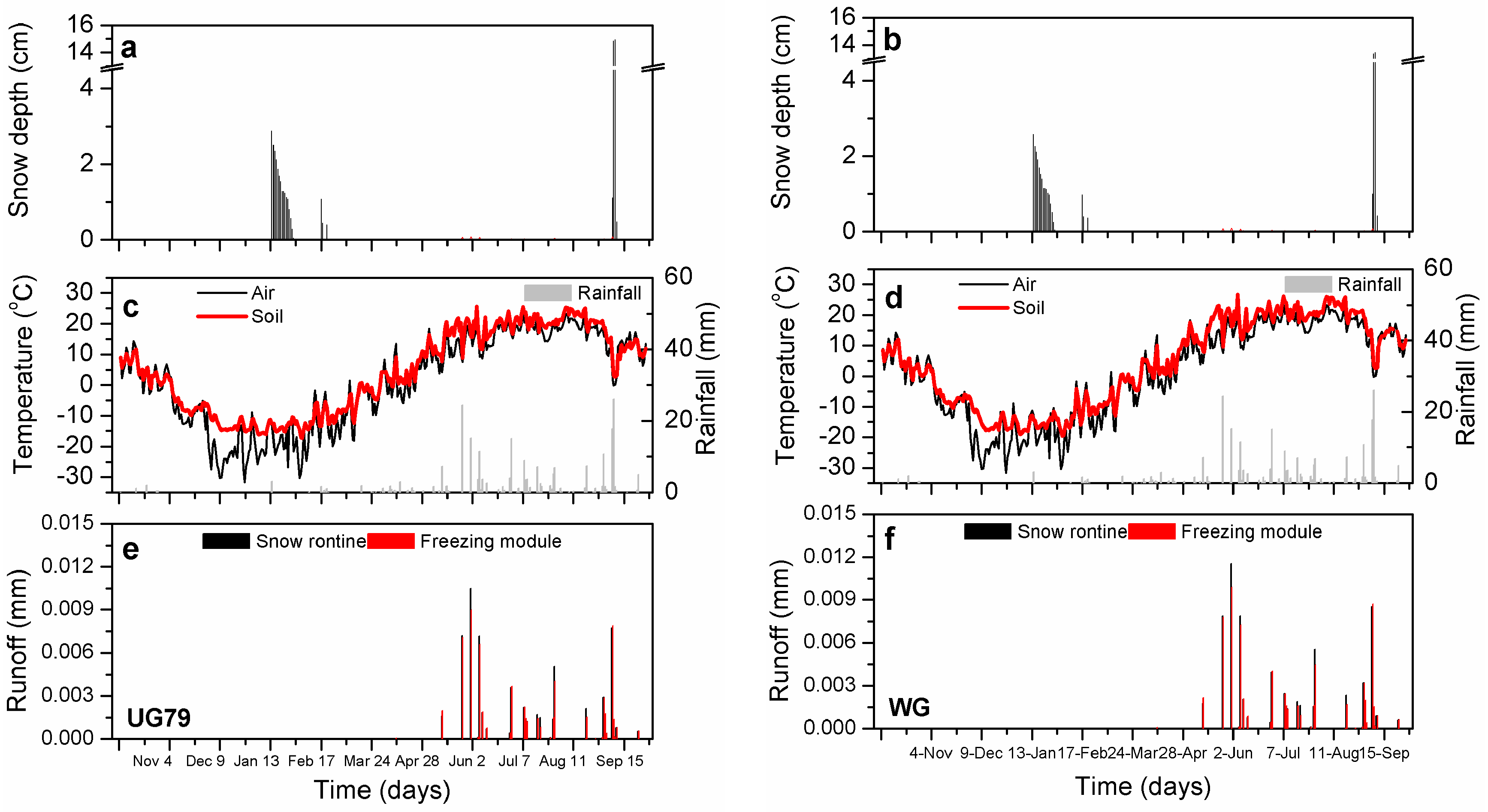
3.3. Simulation of Runoff in Frozen Soil

The temperature threshold at which precipitation is considered to be snow is specified as −2 °C in the normal module of HYDRUS. The normal module predicts up to a 15-cm snow depth (Figure 6a); however, the simulated runoff is negligible when the air temperature is above 0 °C (Figure 6c). This omission is obvious because the normal module does not consider the subsurface soil frozen process, thus discounting for surface runoff above the frozen soil layer. It is likely that surface runoff is generated during snowmelt while soil is fully or at least partially frozen (Figure 6b). Unexpectedly, the freezing module, which can account for the subsurface soil frozen processes, also did not generate surface runoff during winter (Figure 2c). We found that the simulated SWC by the freezing module is higher than the measured values in the transition time when soil begins to thaw (Figure 2a and Figure 4a). This difference implies that the freezing module might overestimate water content and thus underestimate surface runoff during spring snowmelt. Therefore, the freezing module does not seem to be sufficiently sensitive to estimate surface runoff resulting from snowmelt above the frozen soil layer. This shortcoming might relate to the fact that the current freezing module adopts soil surface temperature as the atmospheric boundary condition instead of air temperature and neglects the lag-effects of energy transfer. Consequently, the freezing module may have incorrectly partitioned all of the snowmelt water into infiltration, as both soil thawing and snow melting happen simultaneously. In a real-world situation, the snow melt is controlled by air temperature, whereas the soil thaw is regulated by soil temperature. A transferable boundary condition (e.g., one accounting for air temperature and other accounting for soil temperature) may be suggested so that the surface runoff resulting from snowmelt above the frozen soil layer may be adequately considered. It should also be noted that the gradual release of water (especially ice) from the frozen soil profile increases the soil water infiltration rate and, thus, might also reduce the maximum rate of runoff. A complication at our field sites is that the soil is dry, which may result in a low ice content that allows the melt water to infiltrate easily. The partitioning between surface runoff and frozen soil infiltration is also highly dependent on the selection of the hydraulic soil properties in the model, in particular on the soil hydraulic conductivity. We considered our measured soil hydraulic parameters, as well as the impedance factors as reasonably accurate.

In contrast to the freezing module, an ‘implicit’ frozen soil code that is used in many studies stipulates that the snow melt water has to run off while the soil is still frozen (e.g., [46]). As a result, this stipulation may cause water infiltration to cease inside the soil. Infiltration is only allowed when the frozen soil layer moves downward and the upper soil layer is available for infiltration. In contrast, an ‘‘explicit’’ frozen soil code like the freezing module as we used is theoretically more reasonable as the infiltration rate is dictated by soil temperature, soil ice content and soil hydraulic properties [15]. Frozen soil was expected to have a great influence on the runoff simulation [47]. A previous study by Pitman et al. (1999) did not obtain improved runoff simulation when the soil ice was included in their model. Cherkauer and Lettenmaier [48] also found that the frozen soil module had a relatively small effect on runoff. They explained that the meltwater percolation could occur in the unfrozen topsoil even though snow was present. It is generally accepted that Hortonian surface runoff can always find its way to infiltrate somewhere over a large region because of the spatial variability of soil properties. Although the current freezing soil module has little effect on the simulations of surface runoff, a detailed study of the soil-atmosphere processes and effects of boundary conditions would improve the surface runoff algorithm in the freezing code. Additionally, a 2D simulation may provide more realistic and mechanistic processes of snowmelt water runoff than the 1D simulation used in this study.

3.4. Simulation of Grazing Effects on Soil Freezing and Thawing

In addition to the effects of a frozen soil layer on the water and heat transfer rates, land management also plays a central role in modifying soil hydraulic and thermal parameters through changing the soil structure [49]. Freezing normally reduces the permeability of soils owing to the impeding effect of ice lenses, as well as structural changes. In the grazed sites with a poorly-structured soil [12], freezing often leads to a higher level of aggregation induced by dehydration and the pressure of ice crystals. In contrast, expansion of the freezing soil may have caused the aggregates to break down in the ungrazed sites with a well-structured soil.

Soil water and thermal dynamics were well simulated by the frozen module as a function of grazing management, indicating the model credibility in simulating the land use change. The relatively poor prediction for site WG might be partially attributed to the poor parameterization of the hydraulic parameters that is associated with a platy soil structure created by the growth of ice segregation blades due to winter grazing [19]. Indications that this hypothesis is correct may be observed by a decrease in soil moisture at a 20-cm depth being slower for the WG site than for the UG79 site because of relatively low evaporation attributed to a less continuous pore system for the WG site (Figure 3 and Figure 5). The less continuous pore system for the WG site (Figure 3 and Figure 5) may result in relatively low evaporation, which in turn caused the soil moisture at a 20-cm depth to decrease more slowly in the WG site than in the UG79 site. The decrease in soil moisture at a 5-cm depth after rainfall is slower for the WG site than for the UG79 site since water supplied to the topsoil layer lasts longer for the WG site because of its lower hydraulic conductivity. However, the constant water contents at a 40-cm depth in both sites show that the residual water content is reached and maintained in the deeper layers due to the damped influence either by water infiltration or by soil evaporation. Moreover, the soil water dynamics for the WG site is less responsive to freezing and thawing processes than for the UG79 site. Due to the smaller unsaturated hydraulic conductivity at the WG site, there is greatly reduced moisture migration to the freezing front than at the UG79 site. Consequently, lower water contents were estimated for the WG site than for the UG79 site.

Grazing is the dominant land use for Inner Mongolia grassland where water is normally limited and the soils experience long-term frost periods. Zhao et al. [21] showed that grazing decreased plant available water in summer. In the winter, it is obvious that much less snow trap was associated with the grazed site due to the relatively bare ground as compared to the ungrazed site. The bare ground is frozen more strongly in winter than the ungrazed soil, which further prevented snowmelt infiltration and, consequently, resulted in smaller soil water content at the grazed site even after soil thawing. These model simulations addressed that the soil freezing and thawing processes significantly affected soil water balance, which differed in different treatments. Our findings further imply that the water availability during the summer is also closely associated with water transfer from winter to summer, and winter precipitation stored in the soil provides an important water source for the following growing season. This process strongly influences the local ecohydrological regimes. Thus, understanding and simulating soil freezing and thawing processes are important components of the broader scientific investigation of the impact of future land use change and climate change in cold regions.

4. Conclusions

We compared the normal module of the well-known HYDRUS-1D model with a frozen module that coupled frozen soil processes to show the importance and accuracy of accounting for soil freezing and thawing in the simulation of soil water and heat transfer at a long-term experimental site characterized with a cold and arid climate in the Inner Mongolia grassland (Northern China). The results showed that both the freezing module and the normal module perform very well in estimating the measured soil water and temperature under the unfrozen condition, whereas the freezing module substantially improved the simulation results under the frozen condition. The freezing model performed well in simulating the intraday water phase changes with the dynamics of soil temperature, which to our knowledge is not well reflected by other models. The freezing module did not produce surface runoff generated by snowmelt or soil thawing from the frozen soil layer. We suggest that seasonal water balances, especially considering rainfall water stored as snow, snow drift and the lateral water flow on frozen soil layers, need to be further investigated because of the complicated interactions at the soil-atmosphere interface and, thus, the effects of using the correct boundary conditions during the simulations.

References

1. Saito, H.; Šimůnek, J.; Mohanty, B.P. Numerical analysis of coupled water, vapor, and heat transport in the vadose zone. Vadose Zone J. 2006, 5, 784–800. [Google Scholar] [CrossRef]
2. Zhao, Y.; Nishimura, T.; Hill, R.; Miyazaki, T. Determining hydraulic conductivity for air-filled porosity in an unsaturated frozen soil by the multistep outflow method. Vadose Zone J. 2013. [Google Scholar] [CrossRef]
3. Lewkowicz, A.G.; Kokelj, S.V. Slope sediment yield in arid lowland continuous permafrost environments: Canadian Arctic Archipelago. Catena 2002, 46, 261–283. [Google Scholar] [CrossRef]
4. Bayard, D.; Stahli, M.; Parriaux, A.; Fluhler, H. The influence of seasonally frozen soil on the snowmelt runoff at two Alpine sites in southern Switzerland. J. Hydrol. 2005, 309, 66–84. [Google Scholar] [CrossRef]
5. Harlan, R.L. Analysis of coupled heat-fluid transport in partially frozen soil. Water Resour. Res. 1973, 9, 1314–1323. [Google Scholar] [CrossRef]
6. Flerchinger, G.N.; Saxton, K.E. Simultaneous heat and water model of a freezing snow-residue-soil system I. Theory and development. Trans. ASAE 1989, 32, 565–571. [Google Scholar] [CrossRef]
7. Miller, R.D. Freezing phenomena in soils. In Applications of Soil Physics; Hillel, D., Ed.; Academic Press: New York, NY, USA, 1980; pp. 254–299. [Google Scholar]
8. Hansson, K.; Šimůnek, J.; Mizoguchi, M.; Lundin, L.-C.; van Genuchten, M.T. Water flow and heat transport in frozen soil: Numerical solution and freeze-thaw applications. Vadose Zone J. 2004, 3, 693–704. [Google Scholar] [CrossRef]
9. Wang, L.; Koike, T.; Yang, K.; Jin, R.; Li, H. Frozen soil parameterization in a distributed biosphere hydrological model. Hydrol. Earth Syst. Sci. 2010, 4, 557–571. [Google Scholar] [CrossRef]
10. Zhang, X.; Sun, S.; Xue, Y. Development and testing of a frozen soil parameterization for cold region studies. J. Hydrometeorol. 2007, 8, 690–701. [Google Scholar] [CrossRef]
11. Seyfried, M.S.; Murdock, M.D. Use of air permeability to estimate infiltrability of frozen soil. J. Hydrol. 1997, 202, 95–107. [Google Scholar] [CrossRef]
12. Zhao, Y.; Peth, S.; Horn, R. Modeling of coupled water and heat fluxes in both unfrozen and frozen soils. In Proceedings of the HYDRUS Workshop, Prague, Czech, 28 March 2008; Šimůnek, J., Kodešová, R., Eds.; Czech University of Life Sciences: Prague, Czech Republic, 2008; pp. 55–60. [Google Scholar]
13. Koopmans, R.W.R.; Miller, R.D. Soil freezing and soil water characteristic curves. Soil Sci. Soc. Am. J. 1966, 30, 680–685. [Google Scholar] [CrossRef]
14. Šimůnek, J.; van Genuchten, M.T.; Šejna, M. Recent developments and applications of the HYDRUS computer software packages. Vadose Zone J. 2016. [Google Scholar] [CrossRef]
15. Luo, L.F.; Robock, A.; Vinnikov, K.Y.; Adam Schlosser, C.; Slater, A.G. Effects of frozen soil on soil temperature, spring infiltration, and runoff: Results from the PILPS 2(d) Experiment at Valdai, Russia. J. Hydrometeorol. 2003, 4, 334–351. [Google Scholar] [CrossRef]
16. Wolf, B.; Kiese, R.; Chen, W.; Grote, R.; Zheng, X.; Butterbach-Bahl, K. Modeling N2O emissions from steppe in Inner Mongolia, China, with consideration of spring thaw and grazing intensity. Plant Soil 2012, 350, 297–310. [Google Scholar] [CrossRef]
17. Jansson, P.-E.; Halldin, S. Soil Water and Heat Model: Technical Description; Swedish Coniferous Forest Project. Tech. Rep. 26; Swedish University of Agricultural Sciences: Uppsala, Sweden, 1980. [Google Scholar]
18. Kurylyk, B.L.; Watanabe, K. The mathematical representation of freezing and thawing processes in variably-saturated, non-deformable soils. Adv. Water Res. 2013, 60, 160–177. [Google Scholar] [CrossRef]
19. Krümmelbein, J.; Wang, Z.; Zhao, Y.; Peth, S.; Horn, R. Influence of various grazing intensities on soil stability, soil structure and water balance of grassland soils in Inner Mongolia, P. R. China. In Advances in Geoecology; Horn, R., Fleige, H., Peth, S., Peng, X., Eds.; Catena Verlag: Reiskirchen, Germany, 2006; Volume 38, pp. 93–101. [Google Scholar]
20. Liu, Z.; Yu, X. Coupled thermo-hydro-mechanical model for porous materials under frost action: Theory and implementation. Acta Geotech. 2011, 6, 51–65. [Google Scholar] [CrossRef]
21. Zhao, Y.; Peth, S.; Horn, R.; Krümmelbein, J.; Ketzer, B.; Gao, Y.; Doerner, J.; Bernhofer, C.; Peng, X. Modelling grazing effects on coupled water and heat fluxes in Inner Mongolia grassland. Soil Tillage Res. 2010, 109, 75–86. [Google Scholar] [CrossRef]
22. Zhao, Y.; Peth, S.; Reszkowska, A.; Gan, L.; Krümmelbein, J.; Peng, X.; Horn, R. Response of soil moisture and temperature to grazing intensity in a Leymus chinensis steppe, Inner Mongolia. Plant Soil 2011, 340, 89–102. [Google Scholar] [CrossRef]
23. Ketzer, B.; Liu, H.Z.; Bernhofer, C. Surface characteristics of grasslands in Inner Mongolia as detected by micrometeorological measurements. Int. J. Biometeorol. 2008, 52, 563–574. [Google Scholar] [CrossRef] [PubMed]
24. Iwata, Y.; Hayashi, M.; Suzuki, S.; Hirota, T.; Hasegawa, S. Effects of snow cover on soil freezing, water movement, and snowmelt infiltration: A paired plot experiment. Water Resour. Res. 2010, 46, 1–11. [Google Scholar] [CrossRef]
25. Liu, C.; Holst, J.; Brüggemann, N.; Butterbach-Bahl, K.; Yao, Z.; Jin, Y.; Han, S.; Han, X.; Krümmelbein, J.; Horn, R.; et al. Winter-grazing reduces methane uptake by soils of a typical semi-arid steppe in Inner Mongolia. China Atmos. Environ. 2007, 41, 5948–5958. [Google Scholar] [CrossRef]
26. United States Department of Agriculture. Keys to Soil Taxonomy, 10th ed.Natural Resources Conservation Service, United States Department of Agriculture: Washington, DC, USA, 2006.
27. Steffens, M.; Kölbl, A.; Totsche, K.U.; Kögel-Knabner, I. Grazing effects on soil chemical and physical properties in a semiarid steppe of Inner Mongolia (PR China). Geoderma 2008, 143, 63–72. [Google Scholar] [CrossRef]
28. Hoffmann, C.; Funk, R.; Li, Y.; Sommer, M. Effect of grazing on wind driven carbon and nitrogen ratios in the grasslands of Inner Mongolia. Catena 2008, 75, 182–190. [Google Scholar] [CrossRef]
29. Van Genuchten, M.T. A closed-form equation for predicting the hydraulic conductivity of unsaturated soils. Soil Sci. Soc. Am. J. 1980, 44, 892–898. [Google Scholar] [CrossRef]
30. Lundin, L.-C. Hydraulic properties in an operational model of frozen soil. J. Hydrol. 1990, 118, 289–310. [Google Scholar] [CrossRef]
31. Noborio, K.; McInnes, K.J.; Heilman, J.L. Two-dimensional model for water, heat and solute transport in furrow-irrigated soil: I. Theory. Soil Sci. Soc. Am. J. 1996, 60, 1001–1009. [Google Scholar] [CrossRef]
32. Nimmo, J.R.; Miller, E.E. The temperature dependence of isothermal moisture vs. potential characteristics of soils. Soil Sci. Soc. Am. J. 1986, 50, 1105–1113. [Google Scholar] [CrossRef]
33. De Vries, D.A. The thermal properties of soils. In Physics of Plant Environment; Van Wijk, R.W., Ed.; North-Holland Publishing Company: Amsterdam, The Netherlands, 1963; pp. 210–235. [Google Scholar]
34. Chung, S.; Horton, R. Soil heat and water flow with a partial surface mulch. Water Resour. Res. 1987, 23, 2175–2186. [Google Scholar] [CrossRef]
35. Dall’Amico, M.; Endrizzi, S.; Gruber, S.; Rigon, R. A robust and energy-conserving model of freezing variably-saturated soil. Cryosphere 2011, 5, 469–484. [Google Scholar] [CrossRef] [Green Version]
36. Allen, R.G.; Pereira, L.S.; Raes, D.; Smith, M. Crop Evapotranspiration. Guidelines for Computing Crop Water Requirements; Irrigation and Drainage Paper No. 56; FAO: Rome, Italy, 1998; p. 300. [Google Scholar]
37. Feddes, R.A.; Kowalik, P.J.; Zaradny, H. Simulation of Field Water Use and Crop Yield; John Wiley and Sons: New York, NY, USA, 1978. [Google Scholar]
38. Jarvis, N.J. The MACRO Model (Version 3.1), Technical Description and Sample Simulations; Reports and Dissertations 19; Deptment of Soil Sciences, Swedish University of Agricultural Sciences: Uppsala, Sweden, 1994. [Google Scholar]
39. Zhao, Y.; Huang, M.B.; Horton, R.; Liu, F.; Peth, S.; Horn, R. Influence of winter grazing on water and heat flow in seasonally frozen soil of Inner Mongolia. Vadose Zone J. 2013, 12. [Google Scholar] [CrossRef]
40. Li, H.; Yi, J.; Zhang, J.; Zhao, Y.; Si, B.; Hill, R.; Cui, L.; Liu, X. Modeling of soil water and salt dynamics with shallow water table and its effects on root water uptake in Heihe Arid Wetland, Gansu, China. Water 2015, 7, 2382–2401. [Google Scholar] [CrossRef]
41. Yi, J.; Zhao, Y.; Shao, M.A.; Zhang, J.G.; Cui, L.L.; Si, B.C. Soil freezing and thawing processes affected by the different landscapes in the middle reaches of Heihe River Basin, Gansu, China. J. Hydrol. 2014, 519, 1328–1338. [Google Scholar] [CrossRef]
42. He, H.L.; Dyck, M. Application of multiphase dielectric mixing models for understanding the effective dielectric permittivity of frozen soils. Vadose Zone J. 2013, 12. [Google Scholar] [CrossRef]
43. Zhang, Y.; Treberg, M.; Carey, S.K. Evaluation of the heat pulse probe method for determining frozen soil moisture content. Water Resour. Res. 2011, 47, 143–158. [Google Scholar] [CrossRef]
44. Tian, Z.C.; Heitman, J.; Horton, R.; Ren, T.S. Determining soil ice contents during freezing and thawing with thermo-time domain reflectometry. Vadose Zone J. 2015, 14. [Google Scholar] [CrossRef]
45. Smirnova, T.G.; Brown, J.M.; Benjamin, S.G. Performance of different soil model configurations in simulating ground surface temperature and surface fluxes. Mon. Weather Rev. 1997, 125, 1870–1884. [Google Scholar] [CrossRef]
46. Mitchell, J.F.B.; Warrilow, D.A. Summer dryness in northern mid-latitudes due to increased CO2. Nature 1987, 341, 132–134. [Google Scholar] [CrossRef]
47. Pitman, A.J.; Slater, A.G.; Desborough, C.E. Uncertainty in the simulation of runoff due to the parameterization of frozen soil moisture using the Global Soil Wetness Project methodology. J. Geophys. Res. 1999, 104, 16879–16888. [Google Scholar] [CrossRef]
48. Cherkauer, K.A.; Lettenmaier, D.P. Hydrologic effects of frozen soils in the upper Mississippi River basin. J. Geophys. Res. 1999, 104, 19599–19610. [Google Scholar] [CrossRef]
49. Hillel, D. Environmental Soil Physics; Academic Press: London, UK, 1998; p. 771. [Google Scholar]
Figure 1. (a) Location of the experimental plots with the indication of the dominant northwest wind direction; (b) photographs of the vegetation coverage for the site that has been moderately grazed in winter (WG); and (c) for the site that has been ungrazed since 1979 (UG79). Modified from Hoffmann et al. [28].
Water 08 00424 g001
Figure 2. Measured and simulated soil temperatures, total soil water contents and liquid soil water contents at the 5-cm depth at site UG79 (a) during the hydric year from October 2005 to September 2006; (b) zoomed spring soil melting period; and (c) the zoomed diurnal cycles. M: measured liquid water content; S: simulated total water content running the snow routine; and F: simulated liquid water content running the freezing module.
Water 08 00424 g002
Figure 3. Measured and simulated soil temperatures, total soil water contents and liquid soil water contents for the (a) 20 cm, (b) 40 cm and (c) 100 cm soil depths at site UG79 during the hydric year from October 2005 to September 2006 (M: measured liquid water content; S: simulated total water content running the snow routine; and F: Simulated liquid water content running the freezing module).
Water 08 00424 g003
Figure 4. Measured and simulated soil temperatures, total soil water contents and liquid soil water contents at a 5-cm soil depth at site WG (a) during the hydric year from October 2005 to September 2006; (b) zoomed spring soil melting period; and (c) and the zoomed diurnal cycles. M: measured liquid water content; S: simulated total water content running the snow routine; and F: simulated liquid water content running the freezing module.
Water 08 00424 g004
Figure 5. Measured and simulated soil temperatures, total soil water contents and liquid soil water contents at (a) 20 cm, (b) 40 cm and (c) 100 cm soil depths at site WG during the hydric year from October 2005 to September 2006 (M: measured liquid water content; S: simulated total water content running the snow routine; and F: simulated liquid water content running the freezing module).
Water 08 00424 g005
Figure 6. (a,b) Simulated snow depth; (c,d) air and soil surface temperatures (2 cm) and rainfall; and (e,f) measured runoff at site UG79 and site WG during the hydric year from October 2005 to September 2006.
Water 08 00424 g006