Secondary Currents and Turbulence over a Non-Uniformly Roughened Open-Channel Bed

Abstract

Large-eddy simulations (LES) of the flow over a non-uniformly roughened channel bed are carried out to study the effect of non-uniform bed roughness on turbulence driven secondary currents and turbulence statistics. The channel bed is comprised of alternating rough and smooth strips, the width of which corresponds to the water depth. The Reynolds number based on hydraulic radius and bulk velocity is 34,000. The LES are successfully validated using experimental data. The secondary flow and bed roughness have a significant effect on the streamwise velocity and second order turbulence statistics. Turbulence is enhanced over rough strips and suppressed over smooth strips. Significant lateral momentum transfer takes place due to both advection and turbulence. The bed shear stresses over the smooth strips are approximately four times less than over the rough strips a result of near bed low momentum fluid being transported from the rough strips to the smooth strips and high momentum fluid being convected from the surface towards the bed. The most significant terms in the streamwise momentum equation are quantified and discussed with regard to momentum transfer.

1. Introduction

Secondary currents are considered an important aspect in river engineering because they affect the primary mean flow field, the spanwise variation of bed shear stresses (and consequently the bed and banks erosion), the transport of bed-load and suspended sediments as well as the conveyance and mixing of dissolved matters. In straight open channel flow, secondary currents are a result of turbulence anisotropy (Prandtl’s second kind [1]). Near the water surface, secondary currents transport low momentum fluid from the side walls towards the center of the channel, where high-momentum fluid is suppressed below the free-surface. This triggers a downflow of near surface fluid towards the bed, which results in the velocity dip observed in natural channels (a good summary of early work on this topic is found in Nezu and Nakagawa’s 1993 textbook [2]). The distribution of wall shear stresses along the wetted perimeter in an open-channel is affected by these secondary currents, resulting in local bed shear maxima wherever there is downflow of high momentum fluid and in local bed shear minima wherever there is upward movement (Figure 1). The non-uniform distribution of the wall shear stress in the transverse direction of open channels is important in explaining the longitudinal striping of sediments that has been observed in channels and rivers by Vanoni [3], Culbertson [4], Karcz [5], Colombini [6], and others. On the basis of field observations, Nezu and Nakagawa [7] inferred multi-cellular secondary currents and associated sand ribbons. With Laser Doppler Anemometry (LDA) and an ultrasonic bedform instrument, Nezu et al. [8] and Onitsuka and Nezu [9] found that the organized fluid motions and the associated sediment transport occurred intermittently on a movable plane sand bed and, after the sand ridges were formed, the secondary-current cells appeared stable in the entire channel cross section. Such secondary currents are also generated on beds with smooth and rough striping [10,11,12,13,14]. Gyr and Kinzelbach [15] argue that secondary currents lead to the demixing of sediments in a channel, by transporting fine material laterally towards the smooth strips while maintaining the rough strips through bed amouring. This feedback process further stabilizes the smooth-rough-strip patterns.

Figure 1. Organization of secondary currents in open channel flows, with associated velocity dip regions and bed shear maxima and minima.

Figure 1. Organization of secondary currents in open channel flows, with associated velocity dip regions and bed shear maxima and minima.

Most of the numerical work to date focused on the calculation of secondary currents in closed channels. The first calculation of secondary flow in straight ducts was carried out by Launder and Ying [16], who derived a method that is based on approximating the Reynolds stresses with algebraic expressions by simplifying the corresponding transport equations proposed by Hanjalic and Launder [17]. This model has subsequently been employed, sometimes with modifications, in numerous studies (e.g., [18,19]) to calculate secondary flows in ducts. Recently, new explicit algebraic stress models (EASM) have become popular as an alternative to full Reynolds Stress Models (RSM) to reduce the computational effort [20,21]. A few Direct Numerical Simulation (DNS) studies of flow in ducts exist (e.g., [22,23]). The direct computation of all quantities and the high resolution in space and time allowed these researchers to gain insight into the details of the flow and to investigate the details of the Reynolds stress budgets. Among large-eddy simulations of the flow in square ducts some were performed at similar Reynolds numbers to the DNSs described above (e.g., [24]) and others at much higher Reynolds numbers [25]. A detailed study of flows in narrow ducts with a free surface is provided by Broglia et al. [26]. They investigated the mean flow field and a variety of turbulence statistics and highlighted the complex structure of the flow near the corners formed by the free surface and the side wall. Broglia et al. [26] were able to explain the existence and origination of secondary motions in the context of stress balance equations. Shi et al. [27] performed an LES in a smooth rectangular channel at a Reynolds number of approximately 90,000 and showed that LES allows very accurate predictions of turbulence statistics and boundary shear stress distributions are feasible. Some recent works show the potential of LES to describe the secondary flow patterns and turbulence statistics of curved open-channels (e.g., [28,29,30]). However, flow in bends exhibits different mechanics as the centripetal force contributes to the generation of spanwise motion (Prandtl’s first kind [1]) together with the aforementioned turbulence anisotropy.

Though recent progress has been made to understand turbulence-driven secondary currents in rivers, there are still many knowledge gaps that have to be addressed [31]. In this paper results of an LES of open-channel flow over non-uniformly distributed roughness are reported. LES resolves the energetic, large-scale motion of the flow [32], thus allows to simulate directly flow features created by turbulence, such as the turbulence driven secondary currents to be observed herein. The objectives of this study are to provide a detailed description of turbulence statistics of the flow over a non-uniformly roughened bed, shed light on the generation and virtue of secondary currents and the effect of non-uniform roughness on the bed shear stress, quantify the apparent stress and analyze the streamwise momentum balance. The study intends to further the present level of understanding of the interdependence of secondary currents, turbulence production and anisotrphy, and the distribution of shear stresses momentum in open channel flows.

2. Numerical Framework

The large-eddy simulation code (Hydro3D) used in this study is based on a finite volume discretization on a Cartesian grid with collocated variable arrangement [33] and has been validated thoroughly for many different flows [34,35,36,37,38,39,40,41]. The Hydro3D code solves the filtered Navier-Stokes equations for incompressible fluid flow (e.g., [42]):

$$\frac{\partial {\widehat{u}}_i}{\partial x_i}=0$$

(1)

$$\frac{\partial {\widehat{u}}_i}{\partial t}+\frac{\partial {\widehat{u}}_i{\widehat{u}}_j}{\partial x_j}=-\frac{\partial \widehat{p}}{\partial x_j}+\nu \frac{\partial (2S_{ij})}{\partial x_j}-\frac{\partial {\tau }_{ij}}{\partial x_j}$$

(2)

where ${\widehat{u}}_i$ and ${\widehat{u}}_j$ (i or j = 1, 2, or 3) are the resolved velocity vectors (i.e., ${\widehat{u}}_1=\widehat{u}$, ${\widehat{u}}_2=\widehat{v}$, and ${\widehat{u}}_3=\widehat{w}$ denoting the velocity components in x, y and z axis direction, respectively) and $\widehat{p}$ is the resolved pressure divided by the density. These quantities are filtered in space. Similarly, $x_i$ and $x_j$ represent the spatial location vectors in x, y, and z axis direction, respectively, $\upsilon$ is the kinematic viscosity and $S_{ij}$ is the filtered strain-rate tensor, defined as $S_{ij}$=$\frac{1}{2}\left(\frac{\partial {\widehat{u}}_i}{\partial x_j}+\frac{\partial {\widehat{u}}_j}{\partial x_i}\right)$. The term ${\tau }_{ij}$ results from the unresolved sub-grid scale fluctuations and needs to be modeled by a sub-grid scale (SGS) model. The dynamic version [43] of the original Smagorinsky [44] sub-grid scale (SGS) model is employed to approximate the anisotropic part of ${\tau }_{ij}$, i.e., ${\tau }_{ij}^a$, as ${\tau }_{ij}^a$ = ${\tau }_{ij}-\frac{2}{3}{\delta }_{ij}{k}_r$ ($=-2{\nu }_t{S}_{ij}$), where ${\delta }_{ij}$ is the Kronecker delta and $k_r$ is the residual kinetic energy. An anisotropic filter ($\Delta ={(\Delta x\Delta y\Delta z)}^{1/3}$) together with the characteristic filtered rate of strain ($\left|S\right|={(2S_{ij}{S}_{ij})}^{1/2}$) are used to compute the sub-grid scale eddy viscosity ${\nu }_t$ as ${\nu }_t={(C_s\Delta )}^2\left|S\right|$. The Smagorinsky constant C_s is calculated locally by making use of the flow information available from the smallest resolved scales. A double filtering procedure leads to a closed expression, commonly referred to as Germano’s identity, relating the smallest resolved stresses to the largest unresolved stresses at the two different filter levels. This additional information is then used to determine the model parameter C_s through local averaging. The filtered equations are integrated over finite control volumes and convective and diffusive fluxes are computed using central differences, which ensure second-order accuracy in space. An explicit three-step Runge-Kutta scheme is used to integrate the equations in time providing third-order accuracy.

3. Boundary Conditions and Setup

The computational setup of the LES is selected in analogy to the laboratory experiments of Wang and Chen [1], the data of which are used to validate the LES results. The channel cross-section is divided into alternating rough and smooth strips of width λ, which equals the water depth, h. The channel width to depth ratio is B/h = 8.0 (Figure 2). The roughness in the rough strips is composed of uniform gravel and the relative submergence of the roughness is h/dm = 31, with dm being the mean grain diameter. The Reynolds number based on the hydraulic radius (hr) and the bulk velocity u (bulk) is Re = 34,000. The flow is driven by a pressure gradient dp/dx that unambiguously provides the global shear velocity $u_{*}$ from $\overline{\tau }={dp/dx\cdot h}_r$ and $u_{*}=\sqrt{\overline{\tau }/\rho }$, with $\overline{\tau }$ being the global shear stress.

Figure 2. Cross-sectional view of the setup of the large-eddy simulations (LES).

Figure 2. Cross-sectional view of the setup of the large-eddy simulations (LES).

The computational domain of the simulation spans 16 h in streamwise, 8 h in spanwise and h in the vertical directions, respectively. The streamwise extent is chosen to be big enough to include all relevant turbulence structures, which is verified by performing two-point correlations of the streamwise velocity fluctuation over the smooth strips. This justifies the use of periodic boundary conditions to be applied in the streamwise direction mimicking a fully developed turbulent channel flow. The free surface is set as a frictionless rigid lid and is treated as a plane of symmetry. This treatment is reasonably accurate considering the low Froude number (Fr ≈ 0.35) of the simulation; it is generally accepted that for open channel flows with Froude numbers below approximately 0.5, deformations at the free surface can be considered to be negligibly small and the free surface pressure can be considered to be hydrostatic [45,46,47]. On the smooth strips and the smooth side wall the no-slip condition is applied. The roughness closure model needed to simulate the flow over the roughness employs the method proposed and validated by Stoesser [48]. The bed roughness is incorporated by using a forcing term that is added to the right-hand side of the normalized momentum equations. For the U-equation this force reads in time-discrete form:

$$f=\{\begin{array}{cc}C-D+ \Delta P+\frac{\Delta V}{\Delta t}\left(U_t- U^n\right) & \mathrm{inside} \mathrm{the} \mathrm{roughness}\\ 0& \mathrm{elsewhere}\end{array}$$

(3)

in which C = discrete convection term; D = discrete diffusion term; P = resolved pressure divided by the density; Uⁿ = resolved velocity in streamwise direction in the previous time step; and U_t = target velocity.

Two computational grids were used and only the results of the fine grid simulation are presented and discussed. The fine grid consists of approximately 41 million grid points. The grid is uniform in the horizontal plane using 600, 576 cells in the x and z directions, respectively. The grid spacing in wall units is Δx⁺ ≈ 48 and Δz⁺ ≈ 32, based on the global shear velocity. In the vertical, the grid varies such that it is lowest near the bed and then stretched towards the water surface, where the grid spacing is Δy⁺ ≈ 18. Over the rough strips the vertical spacing is approximately Δy⁺ ≈ 16.0 and over the smooth strips Δy⁺ ≈ 4 .0, which is due to the non-uniform distribution of the wall shear stress across the channel. Figure 3 shows the computational grid in a cross-section (for clarity only every third grid line is plotted). The simulation was initially run for a period of 80 eddy turn-over times, (t_e = h/u_*) to develop the flow and was then continued for another 260 t_e to acquire first and second order statistics.

Figure 3. Cross-sectional view of the fine grid (only every 3rd grid line is plotted).

Figure 3. Cross-sectional view of the fine grid (only every 3rd grid line is plotted).

4. Results and Discussion

4.1. Time-Averaged Flow

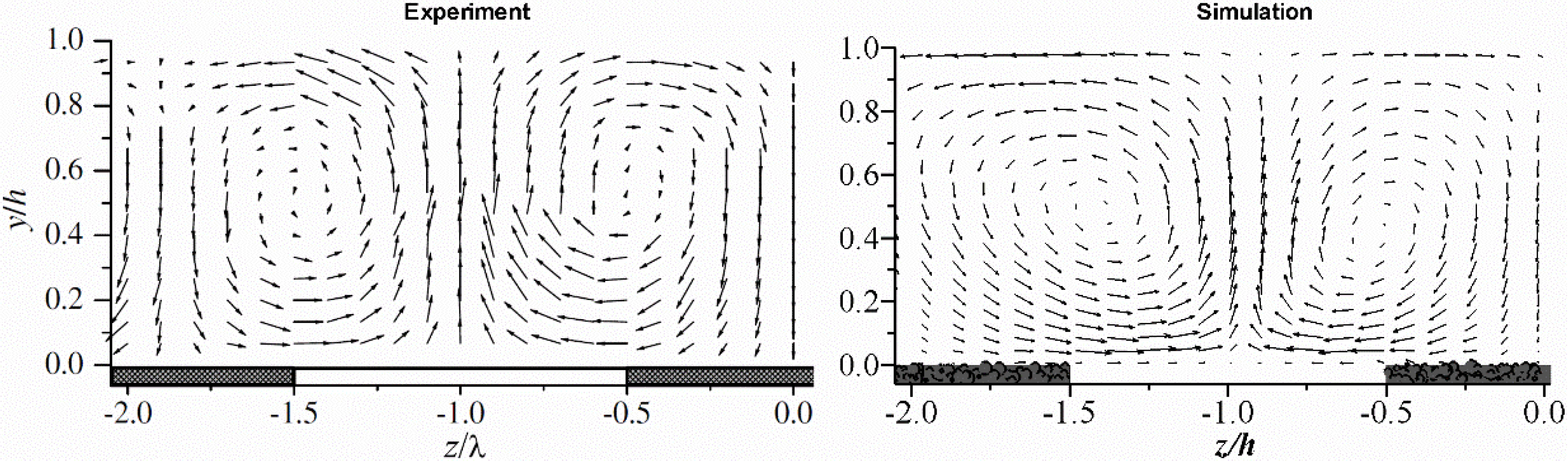
The validation of the LES method employed herein is carried out first by comparing different quantities between the experiment of Wang and Chen [1,2] and the large-eddy simulation. Figure 4 shows measured (a) and calculated (b) secondary currents in a part of the cross-section. The LES predicts accurately the pair of secondary vortices that forms as a result of channel geometry and non-uniform roughness in the cross section. The downward movement of fluid over the rough strips and the upward movement over the smooth strips is matched quite accurately. Some deviations are found in the location of the vortex core and the size of the vortices.

Figure 4. Streamwise-averaged velocity vectors in the vertical-spanwise plane, showing secondary currents: (a) experiment; (b) simulation.

Figure 4. Streamwise-averaged velocity vectors in the vertical-spanwise plane, showing secondary currents: (a) experiment; (b) simulation.

The measured vortex core is at approximately y/h = 0.5, whereas the simulated core is at approximately y/h = 0.4. The measured vortices are almost symmetric whereas the LES predicted vortices differ slightly in size and shape. A possible reason for these slight discrepancies is the rather poor grid resolution in the wall normal direction at the channel side walls. A grid spacing of Δz⁺ ≈ 32 is not considered sufficient to properly resolve the turbulent boundary layer in these regions; wall functions and/or increased near-wall resolution will therefore be implemented in the continuation of the study. However, the overall agreement is quite satisfying. 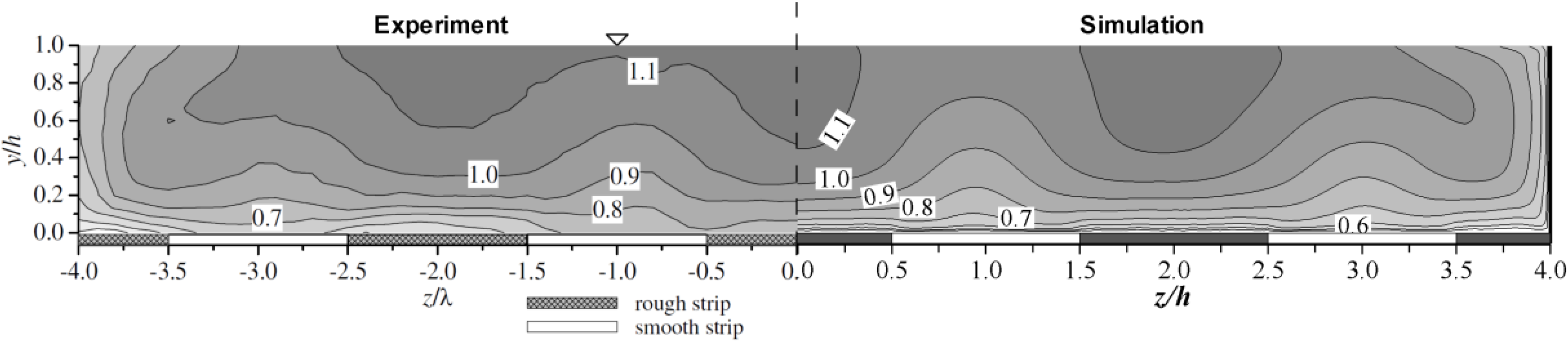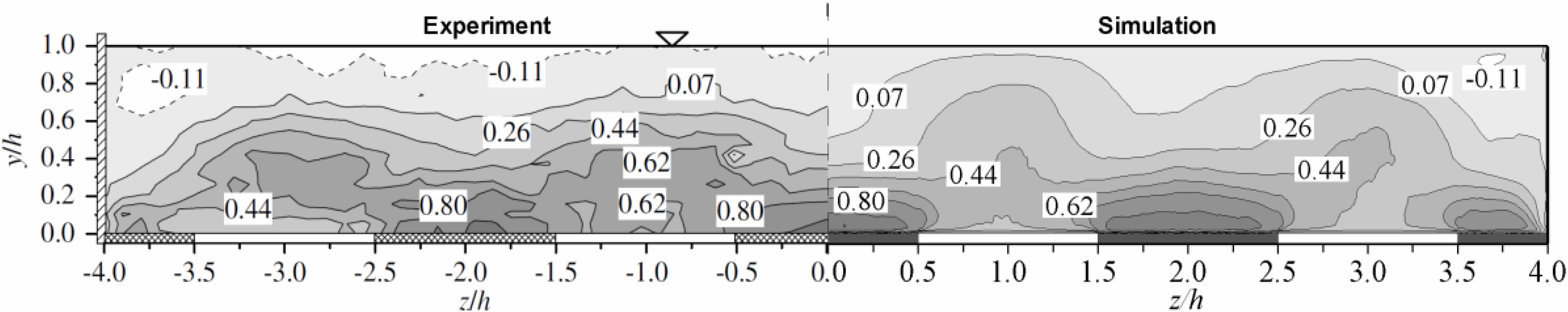Figure 5 presents measured (left part) and calculated (right part) contours of the time-averaged streamwise velocity. Overall the agreement is quite good: simulations and experiments describe quite accurately the location of the high streamwise momentum regions located above the rough strips. The primary flow is influenced strongly by the prevailing secondary currents: The downward movement of high-momentum fluid over the rough strips creates pockets of high streamwise velocity there and the well-known velocity dip. The flow bulges over the smooth strips, which is due to low-momentum near-bed fluid being transported away from the wall. The corner vortex pair causes the flow to bulge towards the corners by transporting high-momentum surface fluid towards the bed-sidewall corner. The differences in this figure and also the ones mentioned above are most likely a result of the modeling inherent in LES, such as the SGS model, the rigid lid assumption, the treatment of roughness or the periodic boundary conditions. This validation of the LES method allows further detailed analysis.

Figure 5. Contours of time-averaged streamwise velocity, normalized on the bulk velocity, for experiments ((left) half of the cross section) and LES (right). The contours provided by the simulation were averaged in the streamwise axis.

Figure 5. Contours of time-averaged streamwise velocity, normalized on the bulk velocity, for experiments ((left) half of the cross section) and LES (right). The contours provided by the simulation were averaged in the streamwise axis.

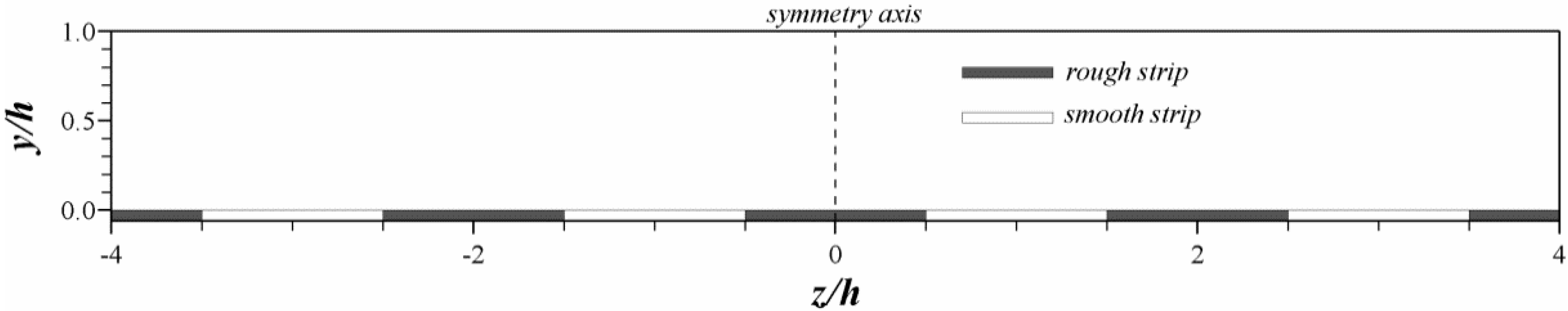
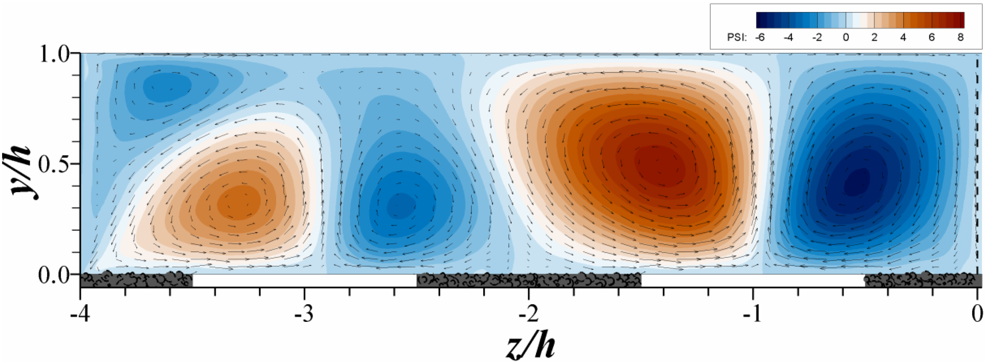
Figure 6 presents velocity vectors and contours of the stream function φ. The flow is symmetric about z/h = 0.0, so for better visibility from now on only the left hand side is shown. Five secondary vortices form in each half of the channel, the shapes of which differ quite significantly from one another. The vortex that is located closest to the centerline rotates clockwise and spans one water depth in both spanwise and wall-normal directions. At the smooth sidewall a corner vortex pair forms with a counter-clockwise rotating vortex near the bed and a clockwise rotating vortex near the free-surface. This vortex pair is not symmetric about the corner-bisector, due to the difference in roughness between the lower (bed-sidewall) and upper (sidewall-free surface) corners. The remaining two vortices have also opposite directions of rotation and differ in size and intensity.

Figure 6. Contours of the streamfunction together with the vectors of the secondary flow in the left half of the cross-section.

Figure 6. Contours of the streamfunction together with the vectors of the secondary flow in the left half of the cross-section.

4.2. Second Order Turbulence Statistics

Figure 7 compares measured (left part) normalized primary shear stresses, $-\overline{u\prime v\prime }/u_{*}^2$, with the one obtained from the simulation (right part). The measurements seem to suffer from insufficient averaging time, however, overall the match is reasonable. The simulation seems to underpredict the positive values of the shear stress found at the free surface in the middle of the channel, which might be a result of the artificial slip boundary condition used in the LES. There is a considerable area of positive shear stress in the side-wall-free-surface-corner, which is predicted correctly by the LES, a result of negative gradients of the streamwise velocity, or the fact that streamwise momentum is transported away from the free surface during inward motion (i.e., u' < 0 and w' < 0), respectively. Near the bed the shear stress is considerably higher above the rough strips than over the smooth strips. 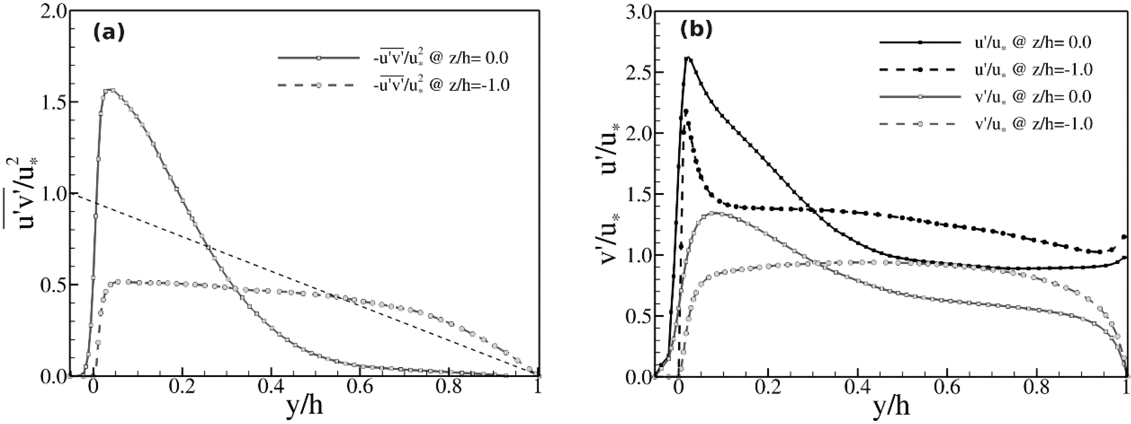The magnitudes of the normalized shear stress over the rough (z/h = 0.0) and smooth strips (z/h = −1.0) in comparison with the theoretical straight line for two-dimensional flows is provided in Figure 7a. The peak of the shear stress over the rough strip is more than 50% greater than the squared mean shear velocity, whilst the shear stress over the smooth strips is suppressed to approximately half of the squared shear velocity. This has two reasons, the first, most obvious one, is that shear stresses are generally higher over rough walls than over smooth walls. The second reason is a result of the prevailing secondary flow. The transport of high momentum towards the bed over the rough strips leads to steeper streamwise velocity gradients there and hence to enhanced shear. The opposite occurs over the smooth strips, where low momentum fluid is convected away from the wall, thereby reducing streamwise velocity gradients. The streamwise and wall-normal turbulence intensity profiles are presented in Figure 8b. They also show that over the rough strip significantly higher values are observed than over the smooth strip. Over the smooth strip the streamwise turbulence intensity profile features a distinct peak (with u'/u_* = 2.2) near the bed. Over the rough strip the peak intensity is about 25% higher (with u'/u_* = 2.6) than over the smooth strip and there is considerable streamwise turbulence until approximately 30% of the water depth (i.e., y/h = 0.3). Interestingly, further away from the bed (i.e., y/h > 0.3) the streamwise turbulence over the smooth strips is slightly higher than over the rough strips. A similar trend is found for the wall normal turbulence intensities.

Figure 7. Contours of measured (left) and simulated (right) shear stress, normalized on the squared global shear velocity, in the cross-section.

Figure 7. Contours of measured (left) and simulated (right) shear stress, normalized on the squared global shear velocity, in the cross-section.

Figure 8. Profiles of the primary shear stress (a) and streamwise and wall normal turbulence intensities (b) over smooth (z/h = −1.0) and rough (z/h = 0.0) strips. In both plots the global shear velocity has been used for normalisation.

Figure 8. Profiles of the primary shear stress (a) and streamwise and wall normal turbulence intensities (b) over smooth (z/h = −1.0) and rough (z/h = 0.0) strips. In both plots the global shear velocity has been used for normalisation.

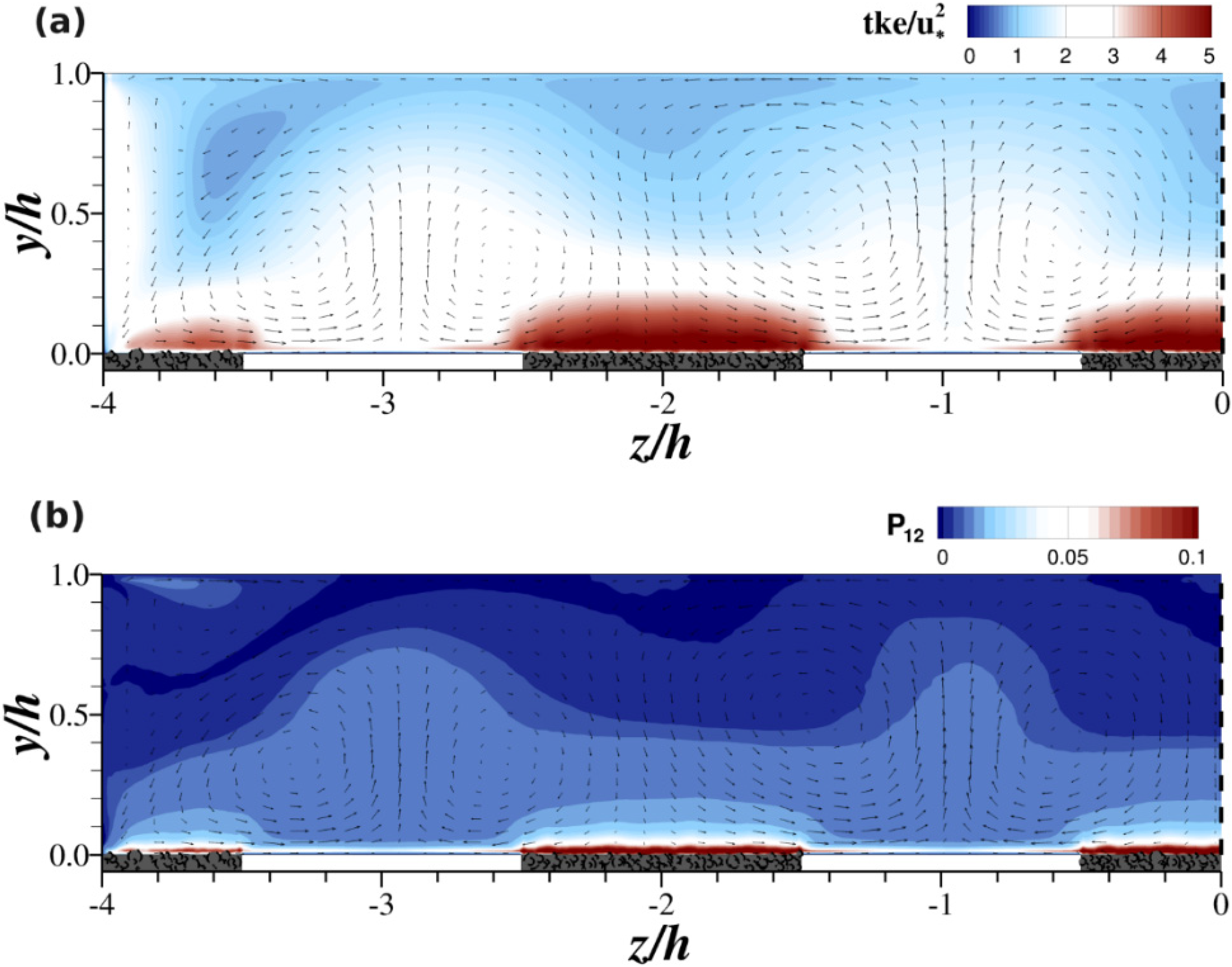
Figure 9a presents contours of the normalized kinetic energy in the left half of the domain, providing a better view of the spatial distribution of turbulence in the cross section. There are pockets of high turbulent kinetic energy over the rough bed, a result of bed roughness but also of the steeper velocity gradients. Turbulence levels, in terms of kinetic energy, over the rough bed are about 70% higher than over the smooth strips and approximately 50% higher than adjacent to the smooth side walls. On the other hand the turbulent kinetic energy decreases much quicker over the rough strips than over the smooth strips, which is owed to the fact that over the smooth strips the wall-normal velocity gradients (i.e., dU/dy) remain throughout the water depth and that the wall-normal Reynolds stress attains non-zero values only very close to the water surface (see Figure 3 and Figure 7). On the other hand over the rough strips dU/dy and $\overline{u\prime v\prime }$ are negligibly small already at approximately half the water depth and dU/dy even becomes negative close to the water surface. Contours of the dominant turbulence production term $\hspace{0.17em}{P}_{12}=-\overline{u\prime v\prime }\frac{\partial U}{\partial y}\hspace{0.17em}$ are plotted in Figure 9b and visualize the statements made above quite well. Clearly, turbulence production occurs mainly over the rough strips, and P₁₂ is relatively small close to the smooth wall. The region of very large P₁₂ values (i.e., P₁₂ larger than about 0.07) extends for between 4 and 6 grid points in the vertical direction above the rough strips, which corresponds to a distance of approximately 16 to 24 wall units.

Figure 9. Contours of the normalized turbulent kinetic energy (a) and normalized dominant turbulence production term (b) in the left half of the cross-section.

Figure 9. Contours of the normalized turbulent kinetic energy (a) and normalized dominant turbulence production term (b) in the left half of the cross-section.

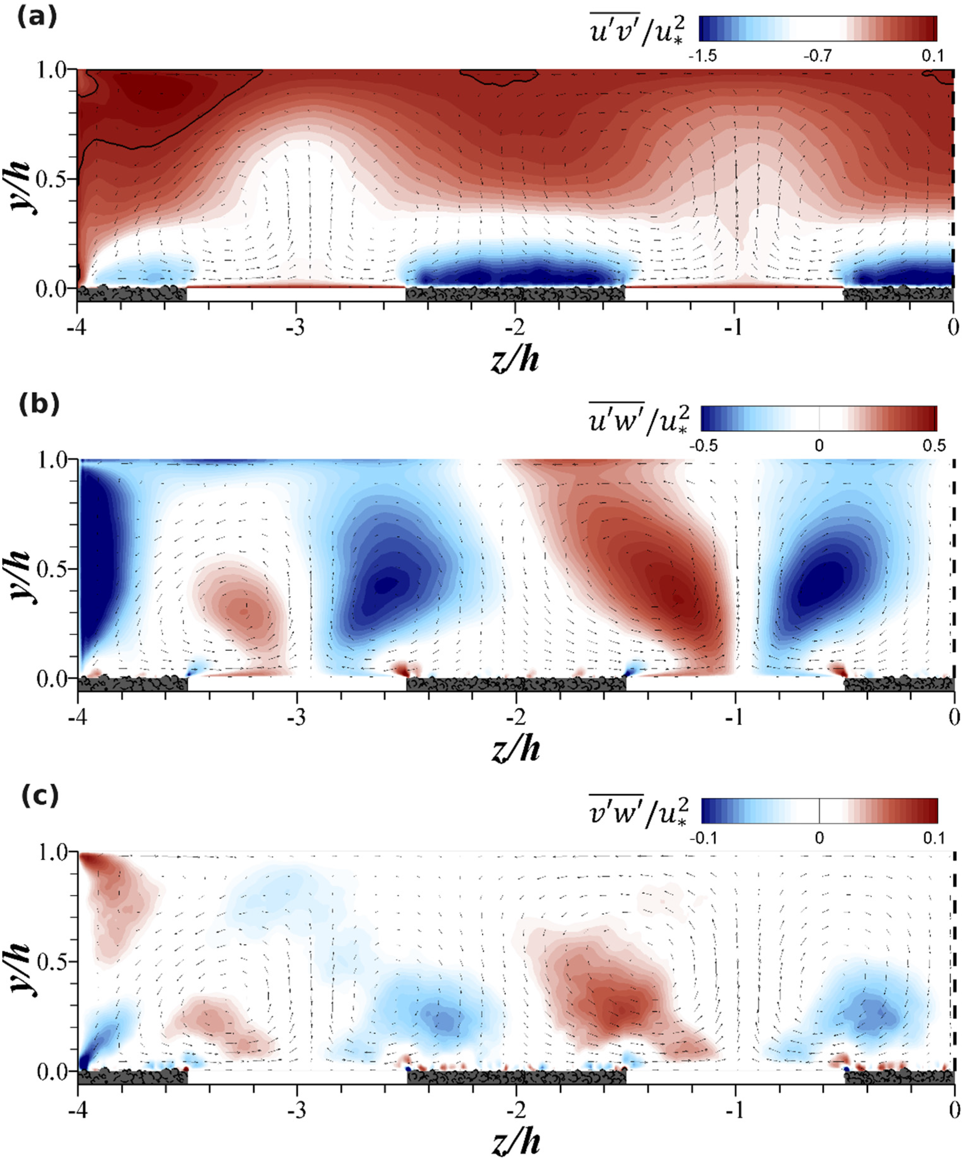
Figure 10 presents the distribution of the three shear stress components together with secondary flow vectors in one half of the cross-section. The primary shear stress, Figure 10a, has been discussed above and its distribution is shown again to highlight interesting features in conjunction with the other two components. Positive $\overline{u\prime v\prime }$ values are found mainly in the free-surface corner but also close to the free surface over the rough strips, which are highlighted by the isoline of $\overline{u\prime v\prime }=0$ (black line). Except very close to the rough wall (where $\overline{u\prime v\prime }$ attain their peaks) spanwise shear stresses, $\overline{u\prime w\prime }$, depicted in Figure 10b, are of comparable magnitude to the primary shear stress and maximum values are observed near the side wall and in the cores of the secondary circulation vortices. This suggests that streamwise momentum transfer in the spanwise direction is quite significant. High values of $\overline{u\prime w\prime }$ are also present at the free surface and near the smooth wall, where W is zero and |V| attains local maxima, indicating streamwise momentum transfer in the spanwise direction by both turbulence and convection. Another interesting feature of the spanwise shear stress is that $\partial \overline{u\prime w\prime }/dz<0$ for upflow, i.e., V > 0, and $\partial \overline{u\prime w\prime }/dz>0$for downflow, i.e., V < 0 (which also applies to flow in smooth bed channels, [4]) and that in areas of dominant or plain up- and downflow. Figure 10c presents cross-plane, or secondary, shear stresses. $\overline{v\prime w\prime }$ reaches local maxima of approximately 10% of the squared shear velocity, which is quite considerable, and are not only found in the channel corners but also at the interface of rough and smooth strips. Significant levels of the secondary shear stress, $\overline{v\prime w\prime }$, and the spanwise shear stress, $\overline{u\prime w\prime }$, are a result of the prevailing secondary currents and, away from the side wall, exhibit a high level of symmetry with respect to the center of the strips (e.g., z/h = 0, z/h = −1.0, z/h = −2.0). This clearly supports the hypothesis that the interplay between secondary currents and cross-stream sediment demixing, i.e., rough-smooth strip formation process as described in [15], leads to a stabilization of such longitudinal bedforms.

Figure 10. Contours of the normalized primary shear stress (a); normalized spanwise shear stress (b) and secondary shear stress (c) in the left half of the cross-section.

Figure 10. Contours of the normalized primary shear stress (a); normalized spanwise shear stress (b) and secondary shear stress (c) in the left half of the cross-section.

The origin of secondary currents was first explained in 1926, when Prandtl [1] suggested that the secondary motion in non-circular ducts was caused by turbulence. He was the first to distinguish between secondary currents that are caused by vortex stretching (first kind) and secondary currents that are generated by the anisotropy of turbulence (second kind). The streamwise vorticity equation is used to describe the origin of secondary currents and can be obtained by eliminating the pressure term in the streamwise component of the momentum equation [49]. For a steady, incompressible, uniform turbulent flow in a straight channel this equation has the exact form [4]:

$$\hspace{0.17em}\hspace{0.17em}\underset{A}{\underbrace{V\frac{\partial \text{Ω}}{\partial y}+W\frac{\partial \text{Ω}}{\partial z}}}=\underset{B}{\underbrace{\frac{{\partial }^2}{\partial y\partial z}\left(\overline{w\prime w\prime }-\overline{v\prime v\prime }\right)}}-\underset{C}{\underbrace{\left(\frac{{\partial }^2}{\partial z^2}-\frac{{\partial }^2}{\partial y^2}\right)\hspace{0.17em}\overline{v\prime w\prime }}}\hspace{0.17em}+\underset{D}{\underbrace{\nu \hspace{0.17em}\left(\frac{{\partial }^2\text{Ω}}{\partial y^2}+\frac{{\partial }^2{\text{Ω}}_1}{\partial z^2}\right)}}$$

(4)

in which ${\text{Ω}}_1\equiv \frac{\partial V}{\partial z}-\frac{\partial W}{\partial y}$ is the streamwise vorticity. Term A represents the convection of streamwise vorticity by the mean flow and D represents the viscous diffusion of Ω. Terms B and C are generation terms of streamwise vorticity and both involve turbulent Reynolds stresses. The origin of secondary currents has been argued about amongst researchers [4,50,51], however, Broglia et al. [26] suggest that in open channels the turbulence anisotropy of the normal stresses (i.e., $\overline{w\prime w\prime }-\overline{v\prime v\prime }$) term dominates the secondary shear stress term in the free surface corner in particular. 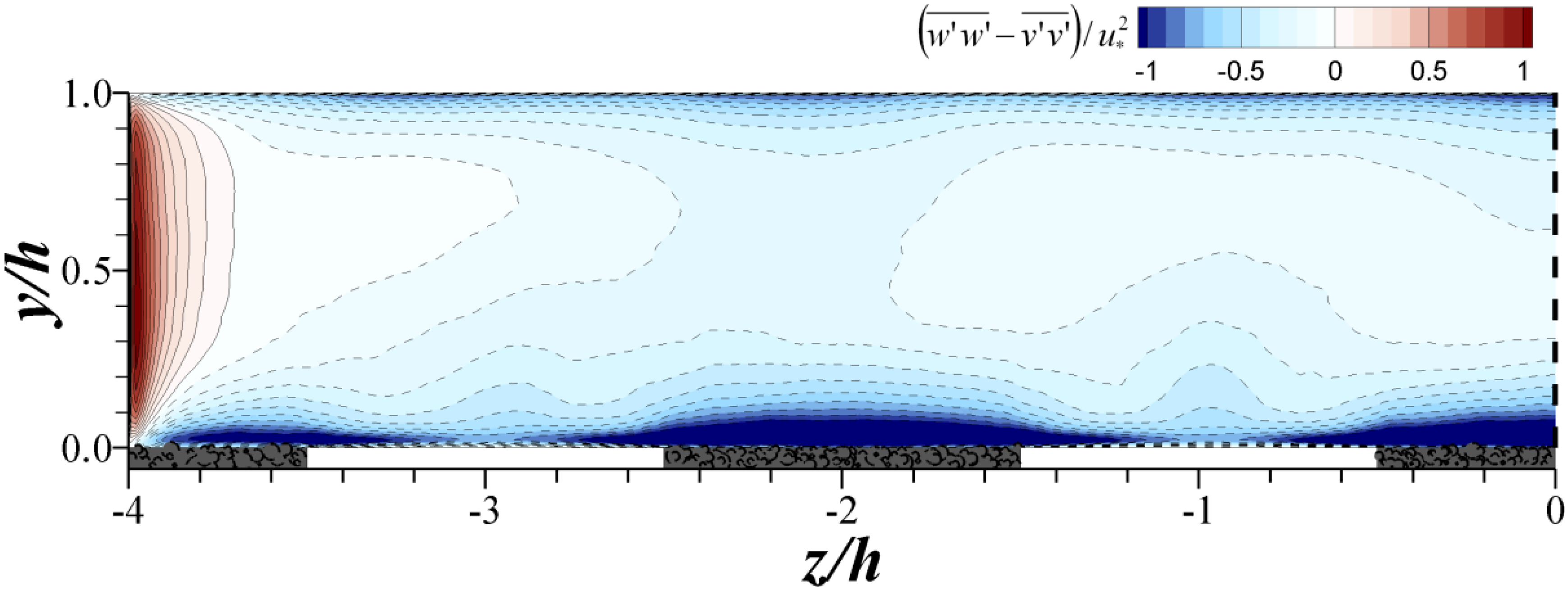Figure 11 presents the distribution of normalized turbulence anisotropy in one half of the domain and supports previous findings which suggest that the secondary currents have their origin in the channel corners, where both $\overline{w\prime w\prime }-\overline{v\prime v\prime }$ and $\overline{v\prime w\prime }$ have local maxima or minima, respectively. The normal stress anisotropy is an order of magnitude greater than the shear stress, and in the corner regions it is of opposite sign. This indicates significant contribution of $\overline{w\prime w\prime }-\overline{v\prime v\prime }$ to streamwise vorticity generation. Substantial gradients of $\overline{w\prime w\prime }-\overline{v\prime v\prime }$ are also found above the rough strips and near the bed at the interface of rough and smooth strips, suggesting that this kind of bedform enhances the generation of secondary currents. In summary, the above discussions showed that secondary currents and the arrangement of non-uniform bed roughness, chosen here, form a closely interrelated system which appears to form stable smooth-rough-strip patterns.

Figure 11. Contours of the normalized normal stress anisotropy in the left half of the domain.

Figure 11. Contours of the normalized normal stress anisotropy in the left half of the domain.

4.3. Bed Shear Stress and Apparent Shear Stress

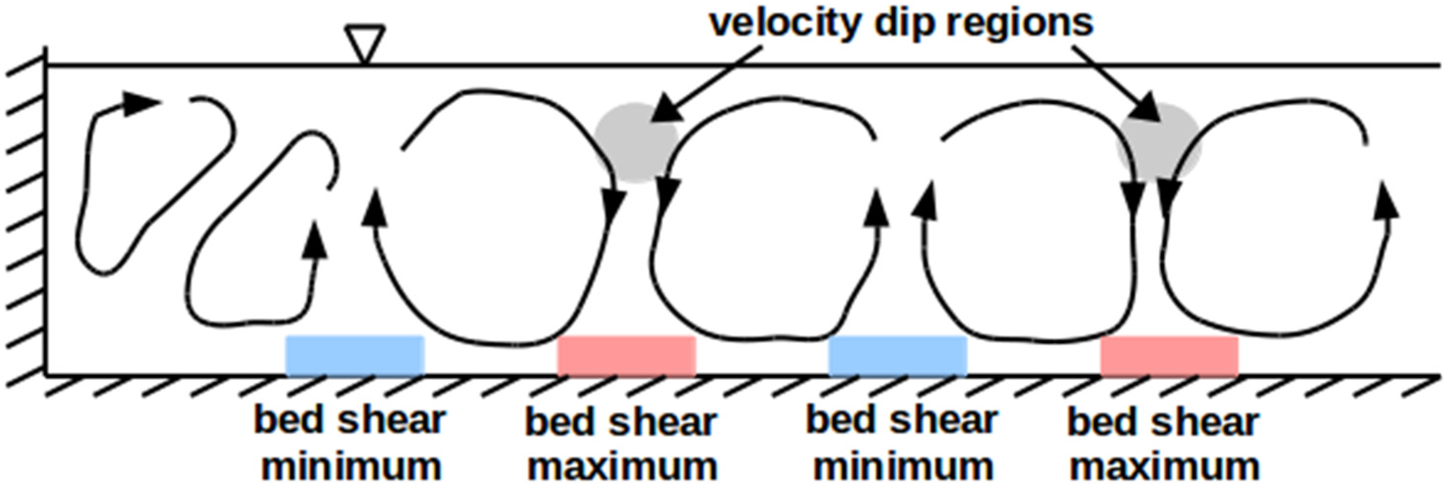
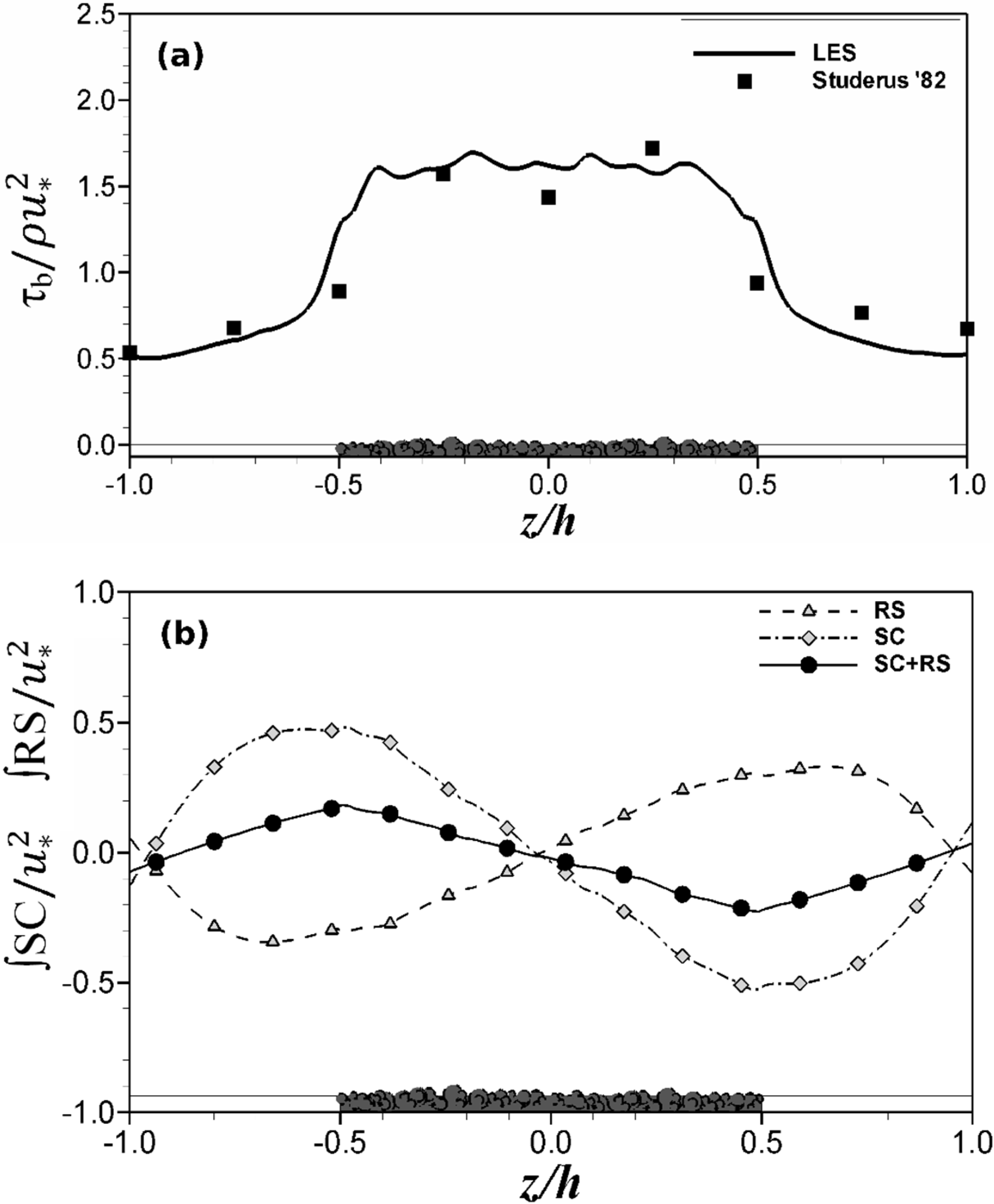
The presence of secondary currents markedly affects the distribution of the wall shear stress along the wetted perimeter of the channel [52,53]: Bed shear stresses are magnified in regions of downflow and are reduced in regions of upflow. The presence of non-uniform bed roughness enhances this pattern, due to the fact that downflow occurs over rough strips where the bed shear stress is naturally greater. Figure 12a presents the spanwise distribution of the normalized bed shear stress, τb$/{\mu }_{*}^2$, in the center section of the channel (i.e., −1 ≤ z/h ≤ 1). The bed-shear stress over the rough bed is obtained from the vertical distribution of $\overline{u\prime v\prime }$, while the bed shear stress over the smooth strips is accurately calculated from the velocity gradient at the first grid point off the wall. Additionally plotted are experimental data of Studerus [13]. Simulation and experimental data agree quite well, though the bed roughness and experimental conditions are not exactly the same. However, the ratio of bedform width to water depth, λ/h, is the same, i.e., λ/h = 1.0, which seems to be the dominant parameter and another indicator of the aforementioned bedform stabilization process. The bed shear stress over the rough strips is about twice as big as the global shear stress, i.e., $\rho {\mu }_{*}^2$, and approximately four times greater than over the smooth strips. Bed shear stress non-uniformity, as a result of sediment demixing, leads to streamwise momentum loss near the rough bed, which has to be compensated for by lateral transport of streamwise momentum via convection and/or turbulence. The presence of secondary currents and non-zero spanwise shear stresses result in the so called apparent stress. The contributions of secondary currents and transverse shear stresses to the squared bulk shear velocity, $u_{*}^2$, can be analyzed with the Reynolds- and depth-averaged streamwise momentum equation, which, for a uniform flow in a straight channel, reads:

$$\hspace{0.17em}\frac{\partial }{\partial z}\hspace{0.17em}\underset{{\displaystyle \int SC}}{\underbrace{{\displaystyle \int UWdy}}}+\hspace{0.17em}\frac{\partial }{\partial z}\underset{{\displaystyle \int RS}}{\underbrace{{\displaystyle \int \overline{u\prime w}\prime dy}}}+\frac{{\tau }_b}{\rho }=u_{*}^2$$

(5)

here the viscous stress contribution is neglected because it is very small except very close to the sidewalls. This equation expresses that the spanwise gradient of the depth integrated secondary current (SC) and Reynolds stress (RS) terms together with the bed shear stress sum to the integral shear velocity, however both ${\displaystyle \int SC}$ and ${\displaystyle \int RS}$ can have opposite signs, so that they may compensate each other. Figure 12b plots the two components of the apparent stress, which are normalized with the squared bulk shear velocity, $u_{*}^2$, in the center section of the channel (i.e., −1 ≤ z/h ≤ 1). The two components have opposite signs over the entire section plotted and the flow is perfectly symmetric about z/h = 0.0, where the two components are zero. Also plotted is the sum of the two, which indicates that the apparent shear stress is mainly carried by the secondary currents except very close to the sidewall, where the viscous stress dominates and ${\displaystyle \int SC}$ approaches zero. The peaks of ${\displaystyle \int SC}$ and ${\displaystyle \int RS}$ do not occur at the same location, and the largest secondary current contribution is approximately half the squared bulk shear velocity and occurs at the interface of rough and smooth channel. The peaks of the Reynolds stress contributions are found a bit further away from the interface and are approximately 40% of the squared bulk shear velocity. The sum of ${\displaystyle \int SC}$ and ${\displaystyle \int RS}$ form a straight line which changes sign at the center of smooth and rough strips and the gradient of the sum changes sign at the interface.

Figure 12. Spanwise distribution of bed-shear stress (a) and apparent shear stress (b) over smooth and rough strips.

Figure 12. Spanwise distribution of bed-shear stress (a) and apparent shear stress (b) over smooth and rough strips.

4.4. Momentum Balance

The transport of streamwise momentum can be analyzed with the Reynolds averaged form of the x-momentum equation, which, for a uniform flow in a straight channel, reads:

$$\hspace{0.17em}\hspace{0.17em}0=\underset{P}{\underbrace{-\frac{1}{\rho }\frac{\partial p}{\partial x}}}\hspace{0.17em}+\underset{V}{\underbrace{\nu \hspace{0.17em}\left(\frac{{\partial }^{2}U}{\partial y^2}+\frac{{\partial }^{2}U}{\partial z^2}\right)}}-\underset{S{C}_1\hspace{0.17em}\hspace{0.17em}+\hspace{0.17em}\hspace{0.17em}S{C}_2}{\underbrace{\left(V\frac{\partial U}{\partial y}+W\frac{\partial U}{\partial Z}\right)}}-\underset{R{S}_1\hspace{0.17em}\hspace{0.17em}+\hspace{0.17em}\hspace{0.17em}R{S}_2}{\underbrace{\hspace{0.17em}\left(\frac{\partial \overline{u\prime v\prime }}{\partial y}+\frac{\partial \overline{u\prime w\prime }}{\partial z}\right)\hspace{0.17em}}}$$

(6)

The two terms denoted SC represent the convective transport of streamwise momentum, term P is the pressure gradient that drives the flow, term RS is transport due to turbulent stresses and term V is transport due to viscous stresses. The latter is negligibly small except very close to the wall. While in a 2D flow, i.e., in the absence of secondary currents only P, V and RS₁ are non-zero, terms SC₁, SC₂ and RS₁ are non-zero in a 3D flow (in the presence of secondary currents). 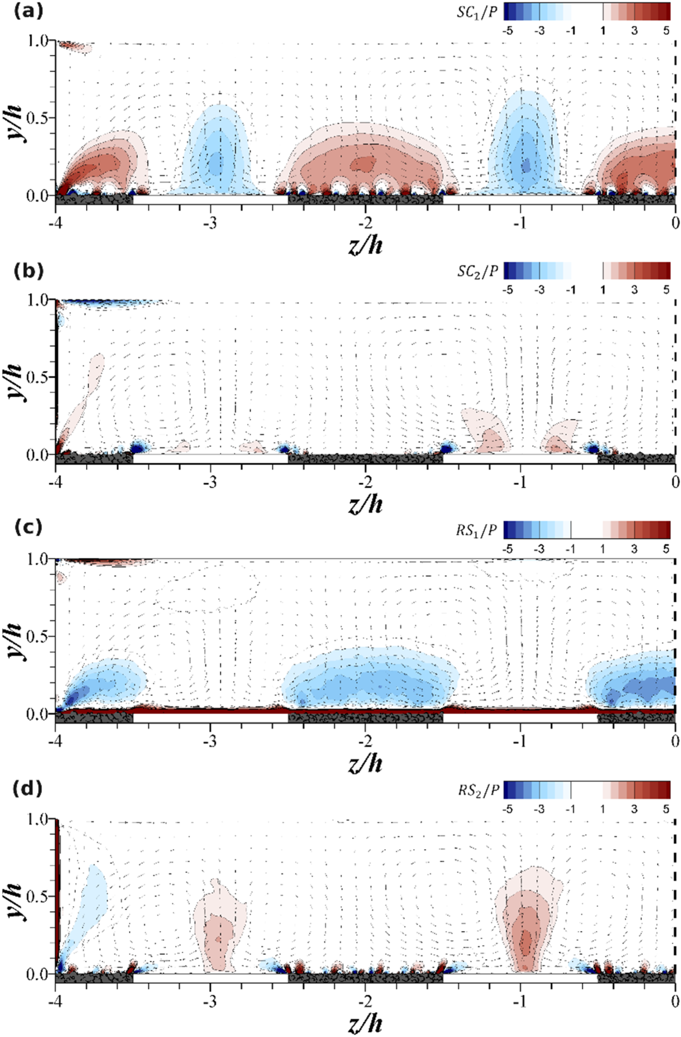The contributions of the four major contributors (i.e., SC₁, SC₂, RS₁, RS₂) to the transport of streamwise momentum are provided in Figure 13. The four components are normalized by P and are all plotted with their respective sign to make obvious which component compensates the other. The contour colors are selected such that small contributions are not visible. First of all, and for obvious reasons, very close to the bed and very close to the sidewall RS₁ and RS₂ dominate the momentum transfer in the flow. Secondly, the above-discussed importance of secondary currents for the transport of streamwise momentum is found in Figure 13, i.e., removal of streamwise momentum over the smooth strips through upflow and addition of streamwise momentum towards the wall through downflow over rough strips (Figure 13a); very small contributions of streamwise momentum through the spanwise shear stress except in the channel corners (Figure 13b); the supression of turbulence away from the rough bed due to the downflow (Figure 13c); and strong lateral gradients of the transverse shear stress in upflow regions over the smooth bed (Figure 13d). Figure 13 also demonstrates which of the four components balances which, and where. For instance transport of streamwise momentum by the secondary currents is compensated by wall normal turbulent transport over the rough strips, while it is compensated by spanwise turbulent transport over the smooth walls. Significant differences are observed in the respective variations of SC₁ and SC₂: these result from the fact that the vertical gradient of streamwise velocity, dU/dy, is generally much larger than the spanwise gradient, dU/dz. It should be noted, however, that near the strip interface there are also strong gradients in the spanwise direction; these are very localized but produce magnitudes of SC₂ that are similar to those of SC₁.

Figure 13. The four dominating components of streamwise momentum transport.

Figure 13. The four dominating components of streamwise momentum transport.

5. Conclusions

Large-eddy simulations of flow in a rectangular channel with non-uniform bed roughness were performed. Setup and boundary conditions were chosen in analogy to a laboratory experiment to ensure code validation and confirmation of the LES’ capability to accurately reproduce such flows. Good agreement between LES and experimental data was found and additional turbulence statistics were extracted from the LES, presented and discussed. The secondary flow together with the non-uniform roughness on the channel bed significantly affects the time-averaged streamwise flow and the second order turbulence statistics. Near the bed, turbulence is enhanced over rough strips and suppressed over smooth strips. The secondary flow and bed roughness affect the streamwise velocity and second order turbulence statistics considerably. Significant lateral momentum transfer takes place due to both advection and turbulence. The bed shear stresses over the smooth strips are approximately four times less than over the rough strips, a result of near bed low momentum fluid being transported from the rough strips to the smooth strips and high momentum fluid being convected from the surface towards the bed. The presence of secondary currents yields nonzero spanwise and cross-plane shear stresses that result in an apparent stress in the spanwise direction and affect the streamwise momentum balance greatly. The naturally high bed shear stress over rough beds is enhanced further by downflow of high-momentum fluid from the surface towards the bed. The generation terms in the streamwise vorticity equation, i.e., normal stress anisotropy and secondary shear stress, are quantified and it was confirmed that turbulence anisotropy gradients dominate over secondary shear stress gradients. Statistical evidence of the feedback process between the secondary flow and bed roughness formation was provided.

References

1. Prandtl, L. Ueber die ausgebildete Turbulenz. In Proceedings of the 2nd International Congress for Applied Mechanics, Zurich, Switzerland, 12–17 September 1926; pp. 62–74.
2. Nezu, I.; Nakagawa, H. Turbulence in Open-Channel Flows. IAHR-Monograph; CRC Press: Rotterdam, The Netherlands, 1993. [Google Scholar]
3. Vanoni, V.A. Transportation of suspended sediment by water. Trans. ASCE 1946, 111, 67–133. [Google Scholar]
4. Culbertson, J.K. Evidence of secondary circulation in an alluvial channel. USGS Prof. Pap. 1967, 575, 214–216. [Google Scholar]
5. Karcz, I. Reflection of the origin of scour: Small-scale longitudinal streambed scours. In Fluvial Geomorphology; Morisawa, M., Ed.; Binghamton State University of New Youk Publications: New York, NY, USA, 1973; pp. 149–173. [Google Scholar]
6. Colombini, M. Turbulence driven secondary flows and the formation of sand ridges. J. Fluid Mech. 1993, 254, 701–719. [Google Scholar] [CrossRef]
7. Nezu, I.; Nakagawa, H. Self-forming mechanism of longitudinal sand ridges and troughs. In Proceedings of the 23rd IAHR Congress, Delft, The Netherlands, 21–25 August 1989; pp. 65–72.
8. Nezu, I.; Nakagawa, H.; Kawashima, N. Cellular secondary currents and sand ribbons in fluvial channel flows. In Proceedings of the 6th Asia and Pacific Division of International Association for Hydraulic Research (APD-IAHR) Congress, Delft, The Netherlands, 26–29 August 1988; pp. 51–58.
9. Onitsuka, K.; Nezu, I. Generation mechanism of turbulence driven secondary currents in open-channel flows. In IUTAM Symposium on Geometry and Statistics of Turbulence; Kluwer Academic: Boston, MA, USA, 2001. [Google Scholar]
10. Wang, Z.-Q.; Chen, N.S. Secondary flows over artificial bed strips. Adv. Water Resour. 2005, 28, 441–450. [Google Scholar] [CrossRef]
11. Wang, Z.-Q.; Chen, N.-S. Time-mean structure of secondary flows in open channel with longitudinal bedforms. Adv. Water Resour. 2006, 29, 1634–1649. [Google Scholar] [CrossRef]
12. McLean, S.R. The role of non-uniform roughness in the formation of sand ribbons. Mar. Geol. 1981, 42, 49–74. [Google Scholar] [CrossRef]
13. Studerus, X. Sekundärströmungen im Offenen Gerinne Über Rauhen Längsstreifen. Ph.D. Thesis, Swiss Federal Institute of Technology, Zurich, Switzerland, March 1982. [Google Scholar]
14. McLelland, S.J.; Ashworth, P.J.; Best, J.L.; Livesey, J.R. Turbulence and secondary flow over sediment stripes in weakly bimodal bed material. J. Hydraul. Eng. 1999, 125, 463–473. [Google Scholar] [CrossRef]
15. Gyr, A.; Kinzelbach, W. Bed forms in turbulent channel flow. Appl. Mech. Rev. 2004, 57, 77–93. [Google Scholar] [CrossRef]
16. Launder, B.E.; Ying, W.M. Secondary flows in ducts of square cross-section. J. Fluid Mech. 1972, 54, 289–295. [Google Scholar] [CrossRef]
17. Hanjalic, K.; Launder, B.E. A Reynolds stress model of turbulence and its application to thin shear flows. J. Fluid Mech. 1972, 52, 609–638. [Google Scholar] [CrossRef]
18. Naot, D.; Rodi, W. Calculation of secondary currents in channel flow. ASCE J. Hydraul. Div. 1982, 108, 948–968. [Google Scholar]
19. Demuren, A.O.; Rodi, W. Calculation of turbulence driven secondary motion in noncircular ducts. J. Fluid Mech. 1984, 140, 189–222. [Google Scholar] [CrossRef]
20. Shih, T.H.; Zhu, J.; Lumley, J.L. A new Reynolds stress algebraic equation model. Comput. Methods Appl. Mech. Eng. 1995, 125, 287–302. [Google Scholar] [CrossRef]
21. Wallin, S.; Johansson, A.V. An explicit algebraic Reynolds stress model for incompressible and compressible turbulent flows. J. Fluid Mech. 2000, 403, 89–132. [Google Scholar] [CrossRef]
22. Gavrilakis, S. Numerical simulation of low-Reynolds-number turbulent flow through a straight square duct. J. Fluid Mech. 1992, 244, 101–129. [Google Scholar] [CrossRef]
23. Huser, A.; Biringen, S. Direct numerical simulation of turbulent flow in a square duct. J. Fluid Mech. 1993, 257, 65–95. [Google Scholar] [CrossRef]
24. Madabhushi, R.K.; Vanka, S.P. Large eddy simulation of turbulence-driven secondary flow in a square duct. Phys. Fluids A 1991, 3, 2734–2745. [Google Scholar] [CrossRef]
25. Su, M.D.; Friedrich, R. Investigation of fully developed turbulent flow in a straight duct with large eddy simulation. J. Fluids Eng. 1994, 116, 677–684. [Google Scholar] [CrossRef]
26. Broglia, R.; Pascarelli, A.; Piomelli, U. Large-Eddy simulations of ducts with a free surface. J. Fluid Mech. 2003, 484, 223–253. [Google Scholar] [CrossRef]
27. Shi, J.; Thomas, T.G.; Williams, J.J.R. Large-eddy simulation of flow in a rectangular open channel. J. Hydraul. Res. 1999, 37, 345–361. [Google Scholar] [CrossRef]
28. Van Balen, W.; Uijttewaal, W.S.; Blanckaert, K. Large-eddy simulation of a mildly curved open-channel flow. J. Fluid Mech. 2009, 630, 413–442. [Google Scholar] [CrossRef]
29. Stoesser, T.; Ruether, N.; Olsen, N.R.B. Calculation of primary and secondary flow and boundary shear stresses in a meandering channel. Adv. Water Resour. 2010, 33, 158–170. [Google Scholar] [CrossRef]
30. Song, C.G.; Seo, I.W.; Kim, Y.D. Analysis of secondary current effect in the modelling of shallow flow in open channels. Adv. Water Resour. 2012, 41, 29–48. [Google Scholar] [CrossRef]
31. Nikora, V.; Roy, A.G. Secondary flows in rivers: Theoretical framework, recent advances and current challenges. In Proceedings of the 7th Gravel-Bed Rivers Conference, Tadoussac, QC, Canada, 6–10 September 2010.
32. Stoesser, T. Large-eddy simulation in hydraulics: Quo Vadis? J. Hydraul. Res. 2014, 52, 441–452. [Google Scholar] [CrossRef]
33. Stoesser, T.; Nikora, V. Flow structure over square bars at intermediate submergence: Large eddy simulation study of bar spacing effect. Acta Geophys. 2008, 56, 876–893. [Google Scholar] [CrossRef]
34. Bomminayuni, S.; Stoesser, T. Turbulence statistics in an open-channel flow over a rough bed. J. Hydraul. Eng. 2011, 137, 1347–1358. [Google Scholar] [CrossRef]
35. Bai, J.; Fang, C.D.; Stoesser, T. Transport and deposition of fine sediment in open channels with different aspect ratios. Earth Surf. Process. Landf. 2013, 38, 591–600. [Google Scholar] [CrossRef]
36. Kara, S.; Stoesser, T.; Sturm, T.W. Turbulence statistics of flow in compound open channels. J. Hydraul. Res. 2012, 50, 482–494. [Google Scholar] [CrossRef]
37. Kara, S.; Stoesser, T.; Sturm, T.W.; Muluhasan, S. Flow dynamics through a submerged bridge opening with overtopping. J. Hydraul. Res. 2015, 53, 282–294. [Google Scholar] [CrossRef]
38. Kara, M.C.; Stoesser, T.; McSherry, R. Calculation of Fluid Structure Interaction: Methods, Refinements, Applications. ICE Proc.: Eng. Comput. Mech. 2015, 168, 59–78. [Google Scholar]
39. Kim, S.; Stoesser, T. Closure modelling and direct simulation of vegetation drag in flow through emergent vegetation. Water Resour. Res. 2011, 47. [Google Scholar] [CrossRef]
40. Kim, D.; Kim, J.H.; Stoesser, T. Hydrodynamics, turbulence and solute transport in ozone contact chambers. J. Hydraul. Res. 2013, 51, 558–568. [Google Scholar] [CrossRef]
41. Fraga, B.; Stoesser, T.; Lai, C.C.K.; Socolofsky, S.A. A large-eddy simulation-based Eulerian-Lagrangian approach to predict bubble plume dynamics. Ocean Model. 2015. submitted for publication. [Google Scholar]
42. Rodi, W.; Constantinescu, G.; Stoesser, T. Large-Eddy Simulations in Hydraulics; CRC Press: Rotterdam, The Netherlands, 2013. [Google Scholar]
43. Germano, M.; Piomelli, U.; Moin, P.; Cabot, W.H. A dynamic subgrid-scale eddy viscosity model. Phys. Fluids 1991, 3, 1760–1765. [Google Scholar] [CrossRef]
44. Smagorinsky, J. General circulation experiments with the primitive equations—Part I: The basic experiment. Mon. Weather Rev. 1963, 91, 99–152. [Google Scholar] [CrossRef]
45. Kirkhill, G.; Constantinescu, G. Flow and turbulence structure around an in-stream rectangular cylinder with scour hole. Water Resour. Res. 2010, 46. [Google Scholar] [CrossRef]
46. Koken, M.; Constantinescu, G. An investigation of the dynamics of coherent structures in a turbulent channel flow with a vertical side-wall obstruction. Phys. Fluids 2009, 21, 085104. [Google Scholar] [CrossRef]
47. Paik, J.; Sotiropoulos, F. Coherent structure dynamics upstream of a long rectangular block at the side of a large aspect ratio channel. Phys. Fluids 2005, 17. [Google Scholar] [CrossRef]
48. Stoesser, T. Physically realistic roughness closure scheme to simulate turbulent channel flow over rough beds within the framework of LES. J. Hydraul. Eng. 2010, 136, 812–819. [Google Scholar] [CrossRef]
49. Einstein, H.A.; Li, H. Secondary currents in straight channels. Trans. Am. Geophys. Union 1958, 39, 1085–1088. [Google Scholar] [CrossRef]
50. Perkins, H.J. The formation of streamwise vorticity in turbulent flow. J. Fluid Mech. 1970, 44, 721–740. [Google Scholar] [CrossRef]
51. Gessner, F.B. The origin of secondary flow in turbulent flow in a corner. J. Fluid Mech. 1973, 58, 1–25. [Google Scholar] [CrossRef]
52. Knight, D.W.; Demetriou, J.D.; Hamed, M.E. Boundary shear in smooth rectangular channels. J. Hydraul. Eng. 1984, 110, 405–422. [Google Scholar] [CrossRef]
53. Nezu, I.; Rodi, W. Experimental study on secondary currents in open channel flow. In Proceedings of the 21st IAHR Congress, Delft, The Netherlands, 13–18 August 1985; pp. 114–119.