Integrated River and Coastal Flow, Sediment and Escherichia coli Modelling for Bathing Water Quality

Abstract

Due to the increasing economic and cultural value of bathing waters and the shellfish industry in the UK and worldwide, water quality in estuarine and coastal waters has attracted considerable public attention in recent years. To obtain accurate predictions of the concentration distributions of faecal indicator organisms (FIOs) in coastal waters for better management of bathing water compliance, it is necessary to build an integrated modelling system to predict the complete diffuse and point source inputs from river and catchment basins. In the present paper, details are given of the development of such an integrated modelling system for simulating the transport and decay processes of FIOs, from catchment areas upstream from the coastal region, in which a distributed catchment module, a 1D river network module and a 2D estuarine and coastal module are linked dynamically by boundary inputs and outputs. Extensive measured data from the catchments, river networks and estuaries have been collated to determine the model parameters. Verification results of the distribution of water levels, flows and velocities, and suspended sediment and Escherichia coli concentrations, at controlled monitoring sites are presented, which show that the integrated model predictions generally agree well with the measurements, although locally appreciable errors can occur. The model results also highlight the importance of including the flux of FIOs via sediments being an important factor in terms of assessing the quality of bathing waters. The main factors influencing the relatively high concentration values in the bathing region are analysed, based on the model predictions and measured data, with four categories of FIO concentration levels being reviewed.

1. Introduction

1.1. Background

Faecal indicator organisms (FIOs), principally coliform organisms and enterococci, are used as surrogate measures of infection risk. These organisms are generally non-pathogenic and excreted by all warm-blooded animals [1]. Escherichia coli (E. coli) and intestinal enterococci are used as the indicators for bathing water quality under the new European Union (EU) Bathing Water Directive (BWD), in line with World Health Organization (WHO) recommendations [2]. Due to the increasing economic and cultural value of bathing waters and the shellfish industry in the UK, together with the high health risks associated with faecal contamination, coastal water quality has attracted increasing public attention over the past two decades or so. A series of infrastructure improvements, together with management measures, such as building and upgrading septic tanks, wastewater treatment plants (WwTPs) and storm overflow structures, etc., have been made over the past 20 years. Field measurements after 2000 have shown that bathing water quality has generally improved in the UK [3]. However, the pace of improvement was slower than initially envisaged, and by 2006 around 5% of bathing waters in the EU still did not comply with the mandatory quality standards [4]. It is uncertain how many bathing water sites can meet the standard required by the new EU Bathing Water Directive (Directive 2006/7/EC) [5]. Meanwhile, in order to find a reasonably accurate solution, field surveys, budget studies [6,7], data mining [8], and process-based modelling investigations [9,10,11] have been undertaken to improve our understanding of the transport and decay processes of FIOs during their journey from source regions, passing through brooks, streams, pipelines, combined sewer overflows (CSOs), WwTPs, river networks, and finally entering the receiving coastal waters [1,7,12]. In our research, an integrated deterministic modelling system has been developed and applied to a large region, including 9 river basins, such as the Ribble, Wyre, Mersey and Lune basins (Figure 1).

1.2. Key Physical, Chemical and Ecological Processes

The transport and decay processes of FIOs from catchment regions to the estuarine and coastal waters mainly involve the following considerations: (1) source apportionment processes in the rural and urban catchments, including both the land surface and soil layers, estimated by livestock and wild animal populations and their age structure, manure collection, storage and spreading, grazing activity and river basin management [13]; (2) FIO die-off and release, driven by intrinsic life processes and environmental factors, such as rainfall, solar radiation, temperature, suspended sediment concentrations (SSCs), soil characteristics, predator population, moisture and nutrition conditions [14,15]; (3) delivery by natural and anthropogenic forcing, with portions of these released FIOs being transported from the landscape through streams and rivers, to the estuary and coastal waters, while anthropogenic activity may change the FIO levels due to land use changes and management measures, e.g., farmland, pasture, arable and ponds, sewage pipes, tanks, CSOs, WwTPs, rivers and estuaries; during transportation, the suspended and bed sediment particles may influence FIO concentration variations by sediment adsorption, desorption and attenuation by radiation [16,17,18]; (4) coupling, integration, evolution and accumulative impact by the conjunction of natural and man-made river systems, and episodic concentration variations driven by extreme events [12].

Figure 1. Maps of study domain, including: (a) the coastal model grid and monitoring sites for the riverine and coastal regions; and (b) the total model domain with catchment stations and coastal bathing sites.

Figure 1. Maps of study domain, including: (a) the coastal model grid and monitoring sites for the riverine and coastal regions; and (b) the total model domain with catchment stations and coastal bathing sites.

1.3. Brief Review of Methods and Models

In recent decades a series of investigations of daily FIO production loads from livestock and wild animals has been undertaken [19], with production estimation methods being reviewed in references [13,20]. Related tools, such as the Bacteria Indicator Tool (BIT) [21] and the Bacteria Source Load Calculator (BSLC) [22], have been developed to estimate the FIO sources and fluxes from catchments into rivers. However, the uncertainly level is often still high because of daily, monthly and seasonal changes in grazing activities [23], manure age [24] and land-use types, etc. When FIOs are left on the land-surface and buried in a shallow soil layer, the rainfall will cause additional losses, with the amount of these losses being primarily influenced by shallow groundwater depths and the rainfall intensity [13]. For the surface loss, the releasing parameter needs to be adjusted according to the grid size, or using other double parameter models, based on the concepts described in Vadas et al. [25]. At the same time, the die-off in the catchment is a key reason for decreasing FIO counts. An exponential model [26] is used extensively for this purpose, wherein the model parameters are adjusted according to the bacteria types and environmental conditions, for example radiation [27,28], moisture [29], soil pH value [30] and vegetation. When detached FIOs in a Hydrologic Response Unit (HRU) enter a pipe, river or estuary, there will be a complex change of FIO concentrations in the surface water column, and potentially via the adsorbed levels in the suspended and bed load sediments. The channel bed can therefore be considered as a transient reservoir of FIOs [31,32]. From these two studies it was found that about 30% of the FIOs were re-suspended from the bed sediments. Results from a similar study [33] showed that under the effects of an artificial flood, generated by breaking a small dam, the E. coli concentration in the water column increased by two orders of magnitude, from a background level of 10² colony forming units (cfu) per 100 mL to over 10⁴ cfu per 100 mL. The in-channel storage level of FIO near the surface of the bed sediments was approximately 10⁸ cfu/m². Wheeler and Burke [34] undertook field investigations which showed that the abundance of FIOs, in the form of Enterococci and E. coli, was 3–38 times higher in the top 20 cm of wetland cores than in the water column, with measurements taken at six freshwater bathing beaches. Passerat and Ouattara [35] produced results that showed that 77% of the E. coli levels in CSOs were due to high levels attached to the suspended particulate matter (SPM). The re-suspension of sewer sediments contributed to 75% of the SPM levels, with the corresponding levels being 10%–70% for E. coli and 40%–80% for intestinal enterococci. Even et al. [36] undertook numerical model tests and recommended that water quality models should take into account CSO inputs in order to be reliable. The linear isotherm and an instantaneous equilibrium of the adsorbing and desorbing processes [37] are usually assumed in simulating the partitioning and attachment of FIOs onto the SPM, because of the complexity of these processes, which may be related to clay content [38], flow velocity and the model cell size.

A comparison between the Soil and Water Assessment Tool (SWAT) and the Hydrologic Simulation Program-Fortran (HSPF) has demonstrated that the predictions from SWAT have a higher level of accuracy than HSPF, because they include estimates of the absorbed bacteria [39]. Meanwhile, the minimal temporal scale of the SWAT and HSPF models is an hour, which is relatively large based on field investigation data, which show that the FIO concentrations may vary significantly within one hour. Many FIO budgets in median [6,40] and highly [41] urbanised catchment regions show that FIO fluxes from sewage networks may provide a large proportion of the total flux, especially during and immediately after an intense rainfall event. Moreover, sewage pipe flows may have higher variations than open channel flows because of their smaller storage volume and human intervention, thus the simple channel flow routing calculation, using the output function in HSPF and the variable storage coefficient method in SWAT [42], appear to be too crude to be used to calculate highly unsteady flow and FIO transport processes in catchments, in spite of their high calculation efficiency and solution stability. Some high-precision numerical methods have been used to solve the highly unsteady flow and related mass transport processes in mountain streams, pipelines and rivers with steep slopes [43,44,45,46]. However, the smaller time step needed for explicit methods may limit the use of such models for complex river and pipe networks. The Preissmann method and slot technique are therefore often adopted for flows in open channel and closed conduits under different flow conditions [47,48,49].

In estuarine and coastal regions, extensive interaction occurs between the FIO transport processes and the river inflows, tides, wind induced waves, sediment transport, etc. Therefore, 2D and 3D models are usually used to simulate FIO transport processes in such water bodies [9,10,17,50,51]. Over the past 20 years, many numerical models have been developed to calculate the FIO transport processes separately, particularly in estuarine and coastal waters. However, it is desirable to integrate the different types of models to achieve a better solution, from the source regions of a catchment and the sewage networks, to rivers, estuaries and coastal basins. Although some commercial software packages, such as MIKE, Infoworks, SWMM and ISIS, have been developed, and various numerical models have been coupled using various linking techniques [52,53], these commercial tools are generally not open-source, and the additional processes for sediment and bacteria coupling cannot easily be calculated using such models. In addition, the integrated models for predicting the FIO transport processes and the fate of FIOs from upstream catchments to the coastal waters are rare.

In the current study an integrated numerical model has been developed based on the concept of C2C (i.e., Cloud to Coast) to predict the transport and fate of FIOs throughout the river basin system. A distributed catchment and river modelling system has been developed to simulate the hydrological, hydraulic and sediment and FIO transport processes. This model is then linked to a refined version of the Environmental Fluid Dynamics Code (EFDC) 2D/3D model. The integrated model is used to calculate the FIO transport processes for the Ribble catchments and river network system, and the downstream estuary and receiving coastal waters, with the Ribble basin being located in the North West of England. The model has been verified using field measurements. Finally, model predictions of E. coli distributions on the catchment surfaces and in soil layers, river and channel flows, suspended sediments and estuarine and coastal waters have been undertaken. The numerical model results are important to produce a reasonably accurate estimate of the parameters governing bathing water concentrations, particularly for better management of bathing waters to meet the future compliance requirements of the EU Water Framework Directive (WFD).

2. Model Details

2.1. Model Grid System

Different HRUs, or grid cells, are used in distributed hydrological models [54]. In the current study a uniform rectangular grid system has generally been used, with some triangular cells being used near irregular catchment boundaries. The calculation domain has been represented by the following three main components:

(1) In a sub-catchment of area ranging from 0.3 to 20 km², a series of rectangular, and some triangular, grid cells with a spatial scale of 250 m × 250 m are included. A sub-channel is used to link the sub-catchments and a series of junctions are used to link the sub-channels;

(2) In the middle and lower regions (MLR), a hybrid river network model has been used, and the results from the distributed model provide point and diffuse sources to the river networks model. If pipelines have been included, they were linked to urban cells, or rural sub-catchments, or sub-channels, and then to the main river channels. The unsteady hydrodynamic and suspended particulate matter transport processes in the networks and pipelines have been solved in the network models. In addition, other natural and man-made domains, such as reservoirs, lakes, CSOs, storage tanks and WwTPs, have been included as appropriate;

(3) In the river, estuary and coastal regions, a refined version of the EFDC-2D model has been used, in which an orthogonal curvilinear grid was used for fitting irregular boundaries. All of the fundamental units have been organised and linked with each other according to some topological rules, which gave good connectivity between the sub-catchments and grid cells, sewer pipelines, junctions etc. In total, the integrated model consists of 2.07 × 10⁵ cells, 6607 sub-catchments, 5112 sub-channels, 5288 junctions and 4.06 × 10⁴ cross-sections. At present the pipelines are not coupled into the integrated model system.

2.2. Catchment Hydrological Model

2.2.1. Hydrological Model in Catchment Cells

The distributed hydrological model used in the current study is based on the Xinanjiang (XAJ) conceptual model [55], which is the most popular rainfall-runoff model in China, and widely used worldwide [56]. The model has 2 sub-models, including: a runoff generation and a routing process sub-model. The Muskingum method is used to route the surface flow component through a sub-catchment, following the path generated by a D8 algorithm [57], while the soil and groundwater flow components are calculated using the linear reservoir method.

The sediment yield and transport equation in catchment cells is given by:

$$\frac{\partial \left(h{S}_k\right)}{\partial t}+\frac{\partial \left(q{S}_k\right)}{\partial x}=Se\left(i,k,t\right)$$

(1)

where t = time, x = distance along the flow direction, h = water depth, q = unit width discharge and S_k = sediment concentration of the kth fraction. The upper boundary condition is S_k(0,k,t) = 0, and the initial condition is S_k(x,k,0) = 0, or an equilibrium concentration is used as the initial condition for the catchment model. Following Alam and Dutta [58], soil erosion estimates consist of the calculation of soil detachment due to rainfall and overland flow.

2.2.2. Sediment Processes in Streams and River Channels

The total-load sediment transport is considered in the current study. The sediment transport Equations [59] in streams are given as follows:

$$\frac{\partial \left(A{S}_k\right)}{\partial t}+\frac{\partial Q_k}{\partial x}+\frac{1}{L_s}\left(Q_k-Q_{*k}\right)=0$$

(2)

$$\left(1-p^{\prime }\right)\frac{\partial \left(A_{bk}\right)}{\partial t}\text{=}\frac{1}{L_s}\left(Q_{tk}-Q_{t*k}\right)=0$$

(3)

Equation (2) can be rewritten as:

$$\frac{\partial Q_k^{n+1}}{\partial x}+p{Q}_k^{n+1}=q$$

(4)

where

$$\begin{array}{c}p=\left(\frac{1}{U_k^{n+1}\mathrm{\Delta }t}+\frac{1}{L_s}\right),q=q_k+\frac{Q_k^n}{U_k^n\mathrm{\Delta }t}+\frac{1}{L_s}{Q}_{*k}\\ Q_k^{n+1}=e^{\overline{p}x}\left(\frac{\overline{q}}{\overline{p}}{e}^{\overline{p}x}+C\right)\end{array}$$

(5)

where L_s = non-equilibrium adaptation length of sediment transport, Q_k = kth size fraction of sediment transport rate in river channel (kg/s), $Q_{t*k}$ = sediment transport capacity (with bed load) in river channel, and C = integration constant.

2.2.3. Distributed Bathing Water Quality Model

The key processes involved in modelling bathing water quality are: (1) to determine the production and distribution of manure, grazing, faecal matter, waste water and the associated concentration of micro-organisms, (2) to simulate the transport of micro-organisms from the land surface to the receiving streams along the hill slope, based on a governing equation similar to Equations (1) and (3), to route the micro-organisms through the stream networks [60].

(1) Production of E. coli

The production and distribution of waste water and the associated concentration of micro-organisms are calculated according to the method obtained from the BIT tools. The main processes and related input data are: (1) livestock density per grid cell; (2) livestock confinement and grazing schedule; (3) access of livestock to streams; (4) manure application rate and timing; (5) location of feedlots, and (6) manure production estimates and waste characteristics. Herein we have assumed that:

$$M_{Surf}={\displaystyle \sum _{i=1}^N\left({\alpha }_{LMN}{M}_{MN}^i+{\alpha }_{LGZ}{M}_{GZ}^i\right)}$$

(6)

$$M_{Soil}={\displaystyle \sum _{i=1}^N\left[\left(1-{\alpha }_{LMN}\right)M_{MN}^i+\left(1-{\alpha }_{LGZ}\right)M_{GZ}^i\right]}$$

(7)

where M_surf, M_soil = counts of FIOs on the land surface and shallow soil at the beginning of time interval Δt (cfu), N = total number of domestic and wild animals on the land, grazing activity is considered only for wild animals and sheep, while both manure and grazing are included for other domestic animals for the arable and pasture land and habitat regions, respectively. $M_{ MN}^{ i}$ and $M_{ GZ}^{ i}$ = the amount of bacteria in the shallow soil layer and land surface, respectively, α_LMN, α_LGZ = coefficients for manure and grazing, with their values being 0.1 and 0.9 in the model respectively, considering that for E. coli the partition ratio between sediment and runoff is generally in the range of 1/9~1/10 [61].

(2) Wash-off E. coli from land surface

Considering the grid size in the distributed model, the modified Bradford and Schijven formula is adopted for the wash-off process for E. coli [61] giving:

$$M_R=M_{Surf}\left[1-{\left(1+k_3\text{β}{R}_S\right)}^{\text{β}}\right]$$

(8)

where k₃ and β = dimensionless fitting parameters, M_surf = amount of bacteria at the surface (cfu), and R_S = runoff depth (cm). According to the formula used in the SWAT model [13] it can be seen that the detached FIO loss will be relatively small when compared to the surface loss. The amount of bacteria released from the soil is calculated using the formula:

$$\mathrm{\Delta }{M}_{Soil}=M_{Soil}{k}_1\mathrm{\Delta }{R}_i$$

(9)

where M_soil = amount of bacteria in the soil at the beginning of time interval $∆t$ (cfu).

(3) Wash-off of the absorbed faecal micro-organisms due to soil loss

The E. coli adsorbed in shallow soil will be transported with the detached soil, and the loads are calculated using the formula:

$$\mathrm{\Delta }{M}_{Eros}=Se\left(i,t\right)\cdot B\cdot \mathrm{\Delta }t\cdot C_P$$

(10)

$$K=K_n+I_{(t)}{K}_s$$

(11)

where K_n = natural die-off rate [d⁻¹], I_(t) = solar radiation [MJ·m⁻²·d⁻¹]; and K_s = solar radiation coefficient [m²·MJ⁻¹].

(1) In the soil, the direct solar radiation component is effectively zero. Nevertheless, the soil moisture level, driven by rainfall and evaporation, will influence the die-off rate. Therefore, the following die-off rate related to soil moisture is used:

$$K=K_n\left[{\alpha }_m+2\left(1-{\alpha }_m\right)\frac{Um-Wu}{Um}\right]$$

(12)

where Um = upper soil water storage maximum thickness, and Wu = upper soil water storage thickness, which is calculated using the distributed hydrological model. Here we assume that the upper soil water storage is half saturated (i.e., $Wu=Um$), then $K=Kn$, in the model, and α_m = 0.4~0.6. When the solar radiation is strong in dry weather the soil soon becomes dry and the radiation will impact indirectly on the die-off rate.

(2) Die-off rate considering the temperature adjustment factor is included as follows:

$$C=C_0{e}^{Kt\text{θ}(T-20)}$$

(13)

where C = concentration at time t; C₀ = initial concentration; t = time [d]; θ = temperature adjustment factor; and T = temperature [ºC].

2.3. River Networks and EFDC 2D Coastal Model

The 1D Saint-Venant equations, solved using the Preissmann scheme, are used for predicting discharges in open-channels and closed conduits, meanwhile the slot technique is adopted for dealing with the drying and wetting processes in river channels [62]. The governing equations and related solution algorithms for predicting the hydrodynamic parameters in estuarine and coastal waters are given in the EFDC help documents [63].

The general transport equation for predicting the concentration distribution of a water quality state variable is given as:

$$\frac{\partial C}{\partial t}=\left(K_B+K_I+K_{Sal}\right){\theta }_W^{T-20}C+\frac{W_C}{V}$$

(14)

where C = concentration of a water quality state variable, $K_c^{New}=\left(K_B+K_I+K_{Sal}\right)$ is the effective total decay rate (per day), K_B = base mortality rate in fresh water at 20 °C under dark conditions without any settling loss; K_sal = mortality rate due to salinity, θ_w = an empirical coefficient for water temperature effects, and T = water temperature. The decay rate due to solar radiation is given as:

$$K_I={\text{α}}_I{I}_0\left(t\right)\frac{1-e^{-K_{e}H}}{K_{e}H}\frac{D}{D_W}$$

(15)

where α_I = coefficient of solar radiation, which is dependent on the type of bacteria, I₀(t) = intensity of solar radiation; K_e = extinction coefficient of light; H = water depth and D and D_w = average distribution coefficients in sediment laden and distilled water, respectively. The ratio D/D_w represents the light intensity attenuation due to sediment suspension. For conciseness, more details relating to the 1D and 2D modelling of bacteria are given in [64]. At present, the distributed hydrological model, the 1D river network model and the EFDC-2D model are all linked by data input and output as boundary conditions or point source inputs. Further development is currently being undertaken to improve the pipe hydrodynamic and water quality sub-models and their linkage with the catchment and riverine hydrodynamic and E. coli transport models.

3. Model Application

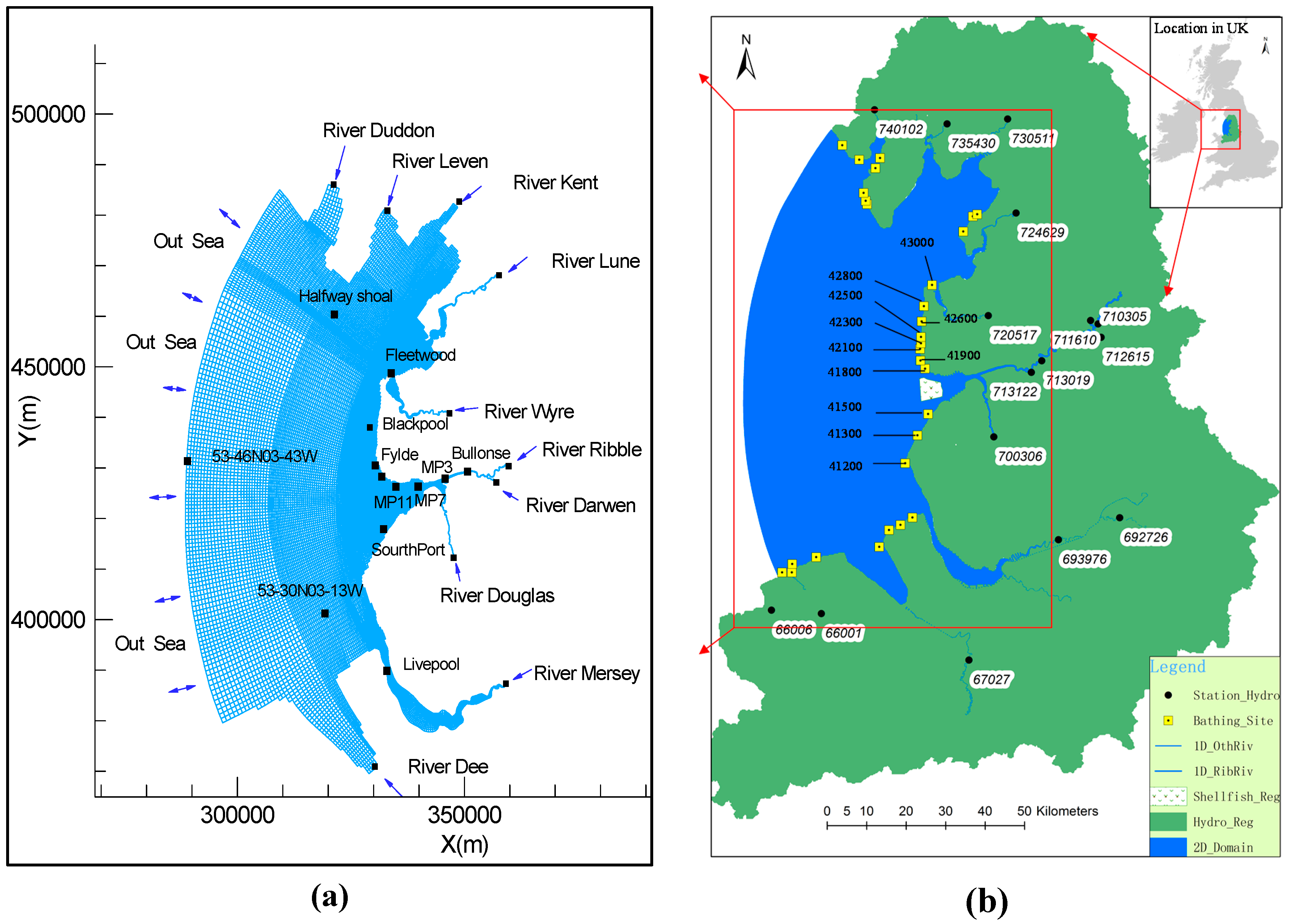
3.1. Study Site

The study domain includes 11 main rivers and catchments that flow into the Irish Sea, including the Clwyd, Dee, Mersey, Ribble, Darwen, Douglas, Wyre, Lune, Kent, Leven and Duddon. Also included are the Morecambe, Duddon, Ribble, Mersey and Dee estuaries, where intense mixing takes place due to the irregular coastline and bathymetry, the large tidal range, the strong currents and wind waves. In considering the strong coupling between the hydrological, hydrodynamic, sediment and E. coli transport processes, all of the 11 river basins and the associated estuarine and coastal waters are included in the integrated model (Figure 1). The catchment and estuary areas are 12,924 and 9664 km², respectively. Moreover, there are 29 national designated bathing beaches in the model domain and a key shellfish harvesting area located in Ribble estuary, with both required to meet the standards set out in the EU Bathing Water Directive 2006/7/EC, and the Shellfish Waters Directive 2006/113/EC [3].

3.2. Data Source and Processing

The data sources, including geographic and topographic data, soil type and properties, land use, meteorologic, hydrologic and hydrodynamic data, sediment and FIO concentration data, etc., are listed in Table 1. In order to use the model system, appropriate data processing has been carried out.

(1) The geographical data are used to decide on the location of the boundary for the 1D and 2D models. The 50 m digital elevation model (DEM) is used to generate the flow direction and topological structures for different cells in the sub-catchments, using the D8 algorithm.

(2) According to the soil classification method of SYMBOL90 in the Harmonized World Soil Database (HWSD) [65], there are 20 types of soils over the model region, with different soil thicknesses, particle size distributions, drainage types, etc. The related soil properties are distributed to the 250 m model grid system via interpolation.

(3) To improve on the model accuracy, the soil parameters at the 250 m hydrological grid system are resolved using the 25 m land cover maps, obtained from the Centre for Ecology and Hydrology, UK. To improve on the comparability of the data collected for different time periods, the 22–24 different classifications used during 1990 and 2000 are unified according to the classifications of LCM 2007, and then simplified further to 10 groups using a correlation analysis. These data are assumed to be uniform within a 25 m grid, which are then used to calculate the percentage of the 10 land use types in each 250 m model grid.

(4) The meteorological data are acquired from two sources: (a) electronic surveying rainfall data at 15 min intervals at 106 stations during 2003–2013 in the model region, obtained from the Environment Agency, UK; and (b) hourly meteorological data at 233 stations, including rainfall, air and earth temperatures, radiation, wind, cloud, pressure, humidity level and sun hour data etc., recorded from 1988 to 2013, and collected by the British Atmospheric Data Centre, UK [66].

(5) The original population and livestock density data in the polygonal shape are interpolated and used in the hydrological model as input data, together with monthly data from the BIT tools. From these data the input FIOs or E. coli counts can be estimated for every cell, at every time step.

Table 1. Data sources used in the model systems.

Database	Purpose	Note (Content and Source)
Geographic Data	Model boundaries	Catchment: [67] River and Ocean: OS1 to 10,000, OS1 to 50,000
Catchment DTM, River networks	Cell slope, flow direction, river generation	(I) 50 m Integrated Hydrological Digital Terrain Model (IHDTM) [68] (II) 1:50,000 Watercourses, River centreline network [69]
Coastal Bathymetry	Grid topography for coastal model	The bathymetric data in the estuary and riverine are merged from 6 data sources and interpolated to the model nodes [64]
Land and river coastal bed sediments	Estuary and riverine bed grain gradation and spatial distribution	(I) Offshore region: Surface sediment distribution data (BGS 1:250,000 V3) ([70]); (II) Riverine: OS maps for the bed sediment type; (III) Nearshore: Sand grain gradation along sandy beach and south part of sea region by Kenneth Pye Associates Ltd [71] with 1566 sampling; (IV) Land: 1000 × 1000 m HWSD soil DEM [65]
Land cover map	Catchment model input	LCM 1990, 2000 and 2007 from Edina: [72]
Climate and meteorological	Meteorological inputs into catchment and coastal model	(I) BADC hourly weather (1989–2013) data including: rainfall, radiation, wind, moisture, temperature and etc. [73] (II) 15 Min rainfall data from EA and Natural Resources Wales (NRW), 68 stations across the model domain.
Discharge data	Model validation and calibration	(I) 15 Min Data from EA and NRW with 30 stations at Ribble catchment and the main 8 controlled stations in the other rivers (II) Daily averaged discharge: [67]
Hydrodynamic	Model lower boundary and verification	Tidal level and current velocity data in 2012 and 2013 measured by the Centre for Research into Environment and Health (CREH), University of Aberystwyth, as part of the Cloud to Coast (C2C) Project
Sediment	Suspended sediment concentrations (SSCs)	(I) SSC measurement in catchment (EA water quality database); (II) SSC in the river Ribble and estuary by CREH in 2012, University of Aberystwyth, as part of C2C, relationship between turbidity (NTU) and SSC(mg/L) is: SSC = 0.51 × NTU (III) SSC data 1997–1999 in the river and estuary from the NERC database
Population and livestock	Population and livestock	(I) Population in 2011 obtained from Office of National Statistics. [74] (II) Livestock and crop areas in 2000 and 2010 across England and Wales. Defra statistics. [75]
CSO, tanks, WwTPs flow and FIO data	Flow and FIO fluxes in urban region, used as point source	From the Infoworks model using results from Pennine Water Group, Dept of Civil and Structural Engineering, University of Sheffield as part of C2C
FIO data	FIO data in River Ribble and estuary and Bathing region	(I) 1999 sample data invested by EA and North West Water Ltd. (II) 2012 sampling, CREH, University of Aberystwyth as part of the C2C. (III) FIO and E. coli in the bathing region (1988–2013) [76]

Table 1. Data sources used in the model systems.

Database	Purpose	Note (Content and Source)
Geographic Data	Model boundaries	Catchment: [67] River and Ocean: OS1 to 10,000, OS1 to 50,000
Catchment DTM, River networks	Cell slope, flow direction, river generation	(I) 50 m Integrated Hydrological Digital Terrain Model (IHDTM) [68] (II) 1:50,000 Watercourses, River centreline network [69]
Coastal Bathymetry	Grid topography for coastal model	The bathymetric data in the estuary and riverine are merged from 6 data sources and interpolated to the model nodes [64]
Land and river coastal bed sediments	Estuary and riverine bed grain gradation and spatial distribution	(I) Offshore region: Surface sediment distribution data (BGS 1:250,000 V3) ([70]); (II) Riverine: OS maps for the bed sediment type; (III) Nearshore: Sand grain gradation along sandy beach and south part of sea region by Kenneth Pye Associates Ltd [71] with 1566 sampling; (IV) Land: 1000 × 1000 m HWSD soil DEM [65]
Land cover map	Catchment model input	LCM 1990, 2000 and 2007 from Edina: [72]
Climate and meteorological	Meteorological inputs into catchment and coastal model	(I) BADC hourly weather (1989–2013) data including: rainfall, radiation, wind, moisture, temperature and etc. [73] (II) 15 Min rainfall data from EA and Natural Resources Wales (NRW), 68 stations across the model domain.
Discharge data	Model validation and calibration	(I) 15 Min Data from EA and NRW with 30 stations at Ribble catchment and the main 8 controlled stations in the other rivers (II) Daily averaged discharge: [67]
Hydrodynamic	Model lower boundary and verification	Tidal level and current velocity data in 2012 and 2013 measured by the Centre for Research into Environment and Health (CREH), University of Aberystwyth, as part of the Cloud to Coast (C2C) Project
Sediment	Suspended sediment concentrations (SSCs)	(I) SSC measurement in catchment (EA water quality database); (II) SSC in the river Ribble and estuary by CREH in 2012, University of Aberystwyth, as part of C2C, relationship between turbidity (NTU) and SSC(mg/L) is: SSC = 0.51 × NTU (III) SSC data 1997–1999 in the river and estuary from the NERC database
Population and livestock	Population and livestock	(I) Population in 2011 obtained from Office of National Statistics. [74] (II) Livestock and crop areas in 2000 and 2010 across England and Wales. Defra statistics. [75]
CSO, tanks, WwTPs flow and FIO data	Flow and FIO fluxes in urban region, used as point source	From the Infoworks model using results from Pennine Water Group, Dept of Civil and Structural Engineering, University of Sheffield as part of C2C
FIO data	FIO data in River Ribble and estuary and Bathing region	(I) 1999 sample data invested by EA and North West Water Ltd. (II) 2012 sampling, CREH, University of Aberystwyth as part of the C2C. (III) FIO and E. coli in the bathing region (1988–2013) [76]

3.3. Key Parameters Related to Hydrological, Hydrodynamic and FIO Transport Processes

In the present model, there are some key parameters that may be sensitive to the hydrological processes, sediment yield and transport, E. coli sources, and the fate and delivery of these FIOs. These parameters are listed in Table 2. In the catchment and coastal models a fractional method is used to simulate the transport of non-uniform sediments, in which the sediment particles are divided into 7 grain size groups (i.e., 50, 100, 200, 300, 500, 800 and 1000 μm), with the first 5 groups being considered as suspended sediments and the last 2 groups as bed load sediments. The bed load component in the coastal and estuarine environments are interpolated based on the data collected from more than 2000 sampling points, while in the catchment and river channel bed layers, the soil data are resampled to decide on the sediment particle component, by omitting the influence of historical fluvial processes on the sediment size distribution in the channel bed. In addition, different partitioning coefficients for the 7 groups of sediments are estimated based on the work undertaken by Pachepsky [61] and with different adsorbing capacities for the FIOs being considered.

3.4. Model Validation

Comparisons between the model predicted and measured discharges, suspended sediment and E. coli concentrations are made, and the model performance is assessed using the Root Mean Square Error (RMSE), the Mean Absolute Error (MAE) and the Nash-Sutcliffe coefficient of efficiency (NSE).

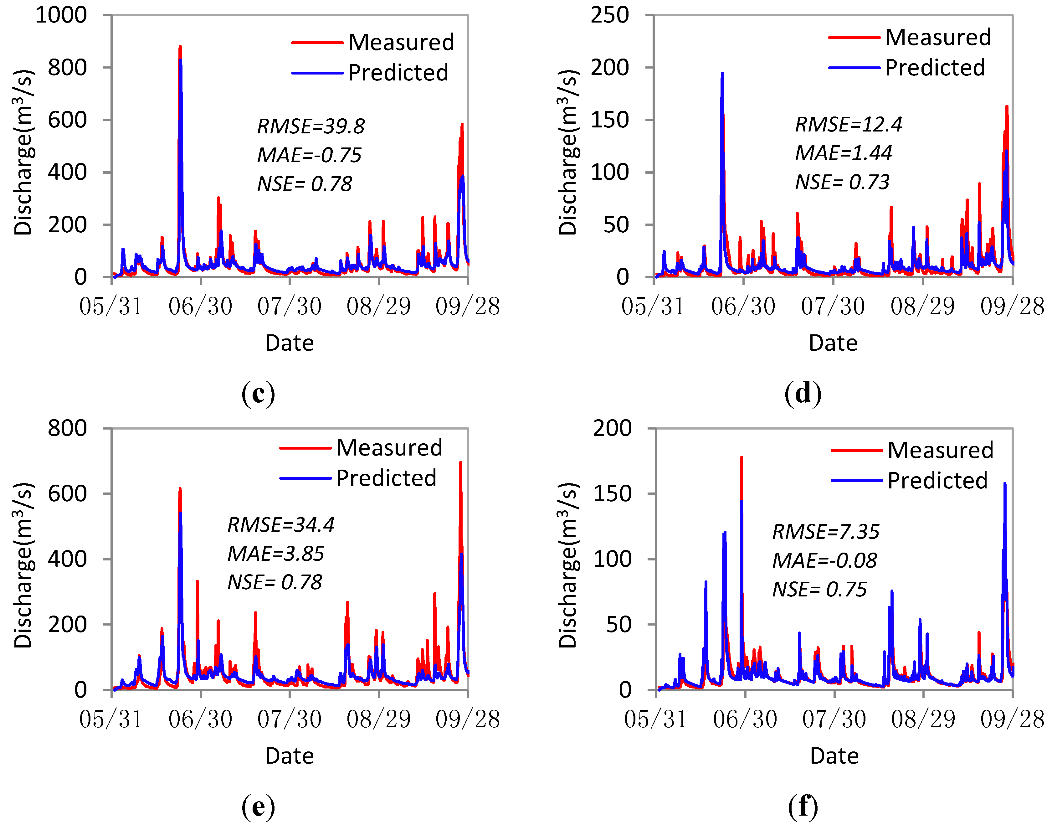
3.4.1. Discharge Verification at Control Gauging Stations

The model predicted discharges for the grid based distributed model, at the 6 main gauging stations shown in Figure 1, are compared with the data measured at 15 min time intervals. From these comparisons it can be seen that the model predicted discharge and phase values agreed well with the measured data (Figure 2). In considering the magnitudes of these discharges they ranged from 0 to 800 m³/s, with the RMSE and MAE values shown in Figure 2 being considered small. Likewise, the NSE value ranged from 0.73 to 0.93, which indicates that the model performance is satisfactory. The errors arise mainly due to the incompleteness of the flow generation modes. In the hydrological model system, the runoff is mainly generated from the saturated storage, thus the model predicted discharge peak is generally lower, and the base flow higher, than the measurements, which indicates that the excess seepage flow component may also be another important source of runoff.

Table 2. Model coefficients and related illustration.

Parameter	Label	Value	Note
Time step in catchment, 1D river and 2D coastal model	$∆t$	300, 30, 2	Time steps for different model(s)
Infiltration rate	IHoton	0.02–0.13	Soil type and land use (m/s)
Impervious area ratio	AlfaIm	0.0–1.0	Land use
Top Soil layer thickness	Um	5–20	HWSD and land use (cm)
Mid soil layer	Lm	20–40	HWSD and land use (cm)
Bottom soil layer	Dm	30–50	HWSD and land use (cm)
Soil particle diameter	Dsed(i)	0.05–1.0	HWSD (mm)
Surface roughness	N	0.03–0.06	HWSD and land use (cm)
Transport time at surface	Ls	0.1–1.0	DEM, HWSD, land use (Hour)
Time in mid soil layer	Li	0.5–10.0	DEM, HWSD, land use (Hour)
Time in bottom soil layer	Lg	3–24.0	DEM, HWSD, land use (Hour)
Time in sub-channel	Lr	0.08–1.0	DEM, HWSD, land use (Hour)
River Bed thickness	ThkBed	0.1, 0.5	Estimation value
Bed sediment composition	DsedBed	50, 100, 200, 300, 500, 1000	Same with closest grid cell (µm)
Manure ratio in surface	αLMN	0.1–0.3	Empirical value varied with manure mode
Grazing feces ratio in surface	αLGZ	0.8–0.9	Empirical value varied with land use
Washing coefficient for soil water	k1	0.1–0.5	Empirical value with different soil
dimensionless fitting parameters	k3	0.2	Washing coefficient in the surface
dimensionless fitting parameters	β	0.5~2.0	Washing coefficient in the surface
Natural die-off rate	Kn	0.5~10	Variation for different habitat
radiation coefficient	KS	1.5	Constant
Moisture coefficient	αm	0.4–0.8	Variation with land use above
Temperature coefficient	θ	1.047	Constant
Sediment partition coefficient	Kd	10~70	Variation with diameter, clay ratio and temperature (mL/g)

Table 2. Model coefficients and related illustration.

Parameter	Label	Value	Note
Time step in catchment, 1D river and 2D coastal model	$∆t$	300, 30, 2	Time steps for different model(s)
Infiltration rate	IHoton	0.02–0.13	Soil type and land use (m/s)
Impervious area ratio	AlfaIm	0.0–1.0	Land use
Top Soil layer thickness	Um	5–20	HWSD and land use (cm)
Mid soil layer	Lm	20–40	HWSD and land use (cm)
Bottom soil layer	Dm	30–50	HWSD and land use (cm)
Soil particle diameter	Dsed(i)	0.05–1.0	HWSD (mm)
Surface roughness	N	0.03–0.06	HWSD and land use (cm)
Transport time at surface	Ls	0.1–1.0	DEM, HWSD, land use (Hour)
Time in mid soil layer	Li	0.5–10.0	DEM, HWSD, land use (Hour)
Time in bottom soil layer	Lg	3–24.0	DEM, HWSD, land use (Hour)
Time in sub-channel	Lr	0.08–1.0	DEM, HWSD, land use (Hour)
River Bed thickness	ThkBed	0.1, 0.5	Estimation value
Bed sediment composition	DsedBed	50, 100, 200, 300, 500, 1000	Same with closest grid cell (µm)
Manure ratio in surface	αLMN	0.1–0.3	Empirical value varied with manure mode
Grazing feces ratio in surface	αLGZ	0.8–0.9	Empirical value varied with land use
Washing coefficient for soil water	k1	0.1–0.5	Empirical value with different soil
dimensionless fitting parameters	k3	0.2	Washing coefficient in the surface
dimensionless fitting parameters	β	0.5~2.0	Washing coefficient in the surface
Natural die-off rate	Kn	0.5~10	Variation for different habitat
radiation coefficient	KS	1.5	Constant
Moisture coefficient	αm	0.4–0.8	Variation with land use above
Temperature coefficient	θ	1.047	Constant
Sediment partition coefficient	Kd	10~70	Variation with diameter, clay ratio and temperature (mL/g)

Figure 2. Hydrological verification of discharge from June to September 2012 for controlled sites (see Figure 1 for locations) at sites: (a) Site 711610 (see Figure 1); (b) Site 713122; (c) Site 713019; (d) Site 720517; (e) Site 724629; (f) Site 730511.

Figure 2. Hydrological verification of discharge from June to September 2012 for controlled sites (see Figure 1 for locations) at sites: (a) Site 711610 (see Figure 1); (b) Site 713122; (c) Site 713019; (d) Site 720517; (e) Site 724629; (f) Site 730511.

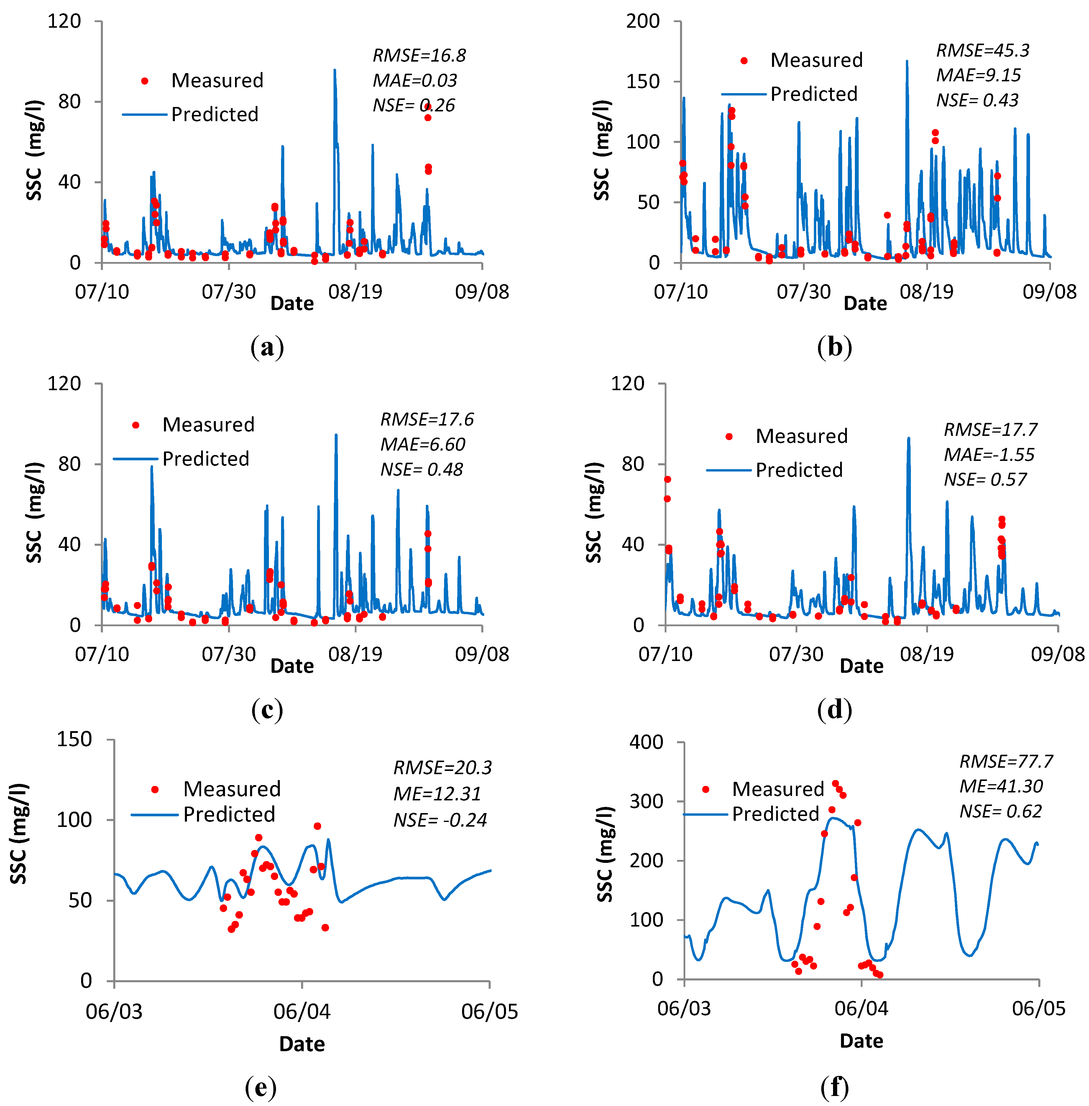
3.4.2. Verification of Sediment Concentration for the River Ribble

Figure 3 shows comparisons between the model predicted and field measured SSCs at 6 sampling points along the Ribble river in 2012 (see Table 1), including the stations along the main reaches of the river basin and including the important branched rivers of: the upper reach of the Ribble (No.710305), the Hodder (No. 711610), the Calder (No.712615), the Darwen (No. 713122), the middle reach of Ribble (No. 713019) and the lower reaches of the Ribble at Bullnose and 11 mile post (MP) (see Figure 1). It can be seen that both the measured and model predicted total SSCs of the 5 sub-groups are highly variable in the upper reaches of the Ribble, and the Calder and Darwen rivers, which may be driven by intensive rainfall, spatial heterogeneity in the soil particle size and properties, and the bed slope. The deviation may also be caused by the different sediment yield methods used for the different land use types. The model predicted SSC values generally agreed well with the measured data along the lower part of the estuary (i.e., at 11MP), while the model predictions did not fit well with the measured values at Bullnose, which is mainly driven by the flow and sediment transport processes upstream and the backwater of the high tide level. In addition, the sediment concentrations at Bullnose may be also driven by the spatially non-uniform bed sediment size distributions. The sediment particles from the upper boundary are predicted to deposit along the middle reach of the Ribble main channel, i.e., from Bullnose to 3MP, because of the smaller channel longitudinal bed slope, the wide saltmarsh and the low flow velocity arising from the action of the tide. While in the Ribble estuary, the high sediment concentrations are mainly caused by re-suspension of the fine sediment particles and the transport caused by the river flow and the tide, with the concentration variations being reasonably accurately predicted in the estuary. The measured and model predicted results at Bullnose and 11MP show that the fine sediment concentrations in the estuary are mainly controlled by the sediment supply from the coast and re-suspension of local fine particles at the interface between the river and estuary, with the sediment flux from the rivers generally being of secondary importance, especially for medium and low inflows.

Figure 3. Suspended sediment concentrations (SSCs) verification at 4 monitoring sites along the river Ribble in 2012 and 2 riverine and coastal sites in 1999 (see Figure 1 for locations) at sites: (a) Site 710305 (see Figure 1); (b) Site 713122; (c) Site 711610; (d) Site 713019; (e) Site Bullnose; (f) Site MP11.

Figure 3. Suspended sediment concentrations (SSCs) verification at 4 monitoring sites along the river Ribble in 2012 and 2 riverine and coastal sites in 1999 (see Figure 1 for locations) at sites: (a) Site 710305 (see Figure 1); (b) Site 713122; (c) Site 711610; (d) Site 713019; (e) Site Bullnose; (f) Site MP11.

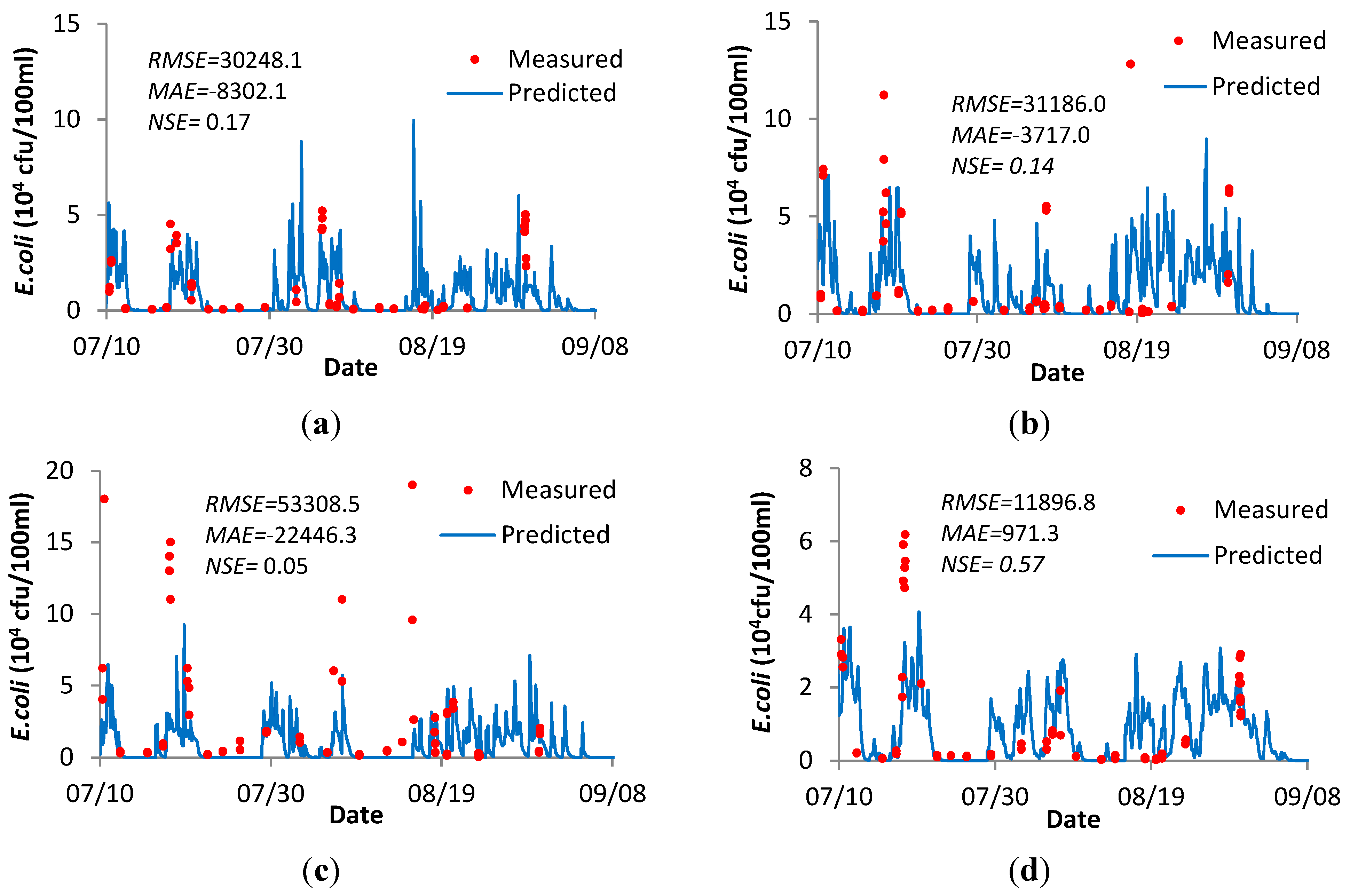
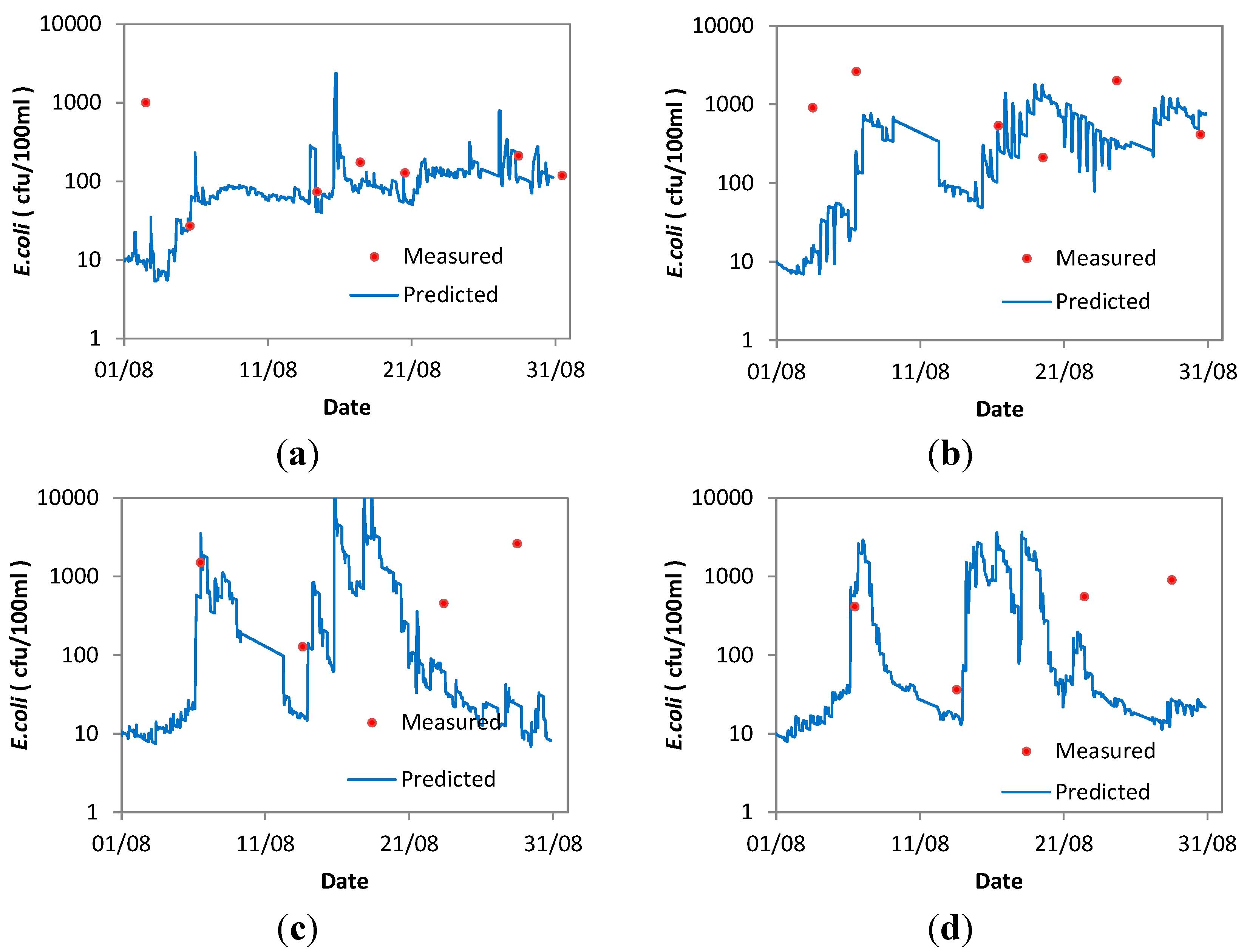
3.4.3. E. coli Verification for the River Ribble and Bathing Region

The E. coli concentration data collected from more than 10 sites in river Ribble and 29 bathing sites along the Fylde coast are used to verify the model. Figure 4 shows comparisons between the model predictions and field data at 4 sites located along the river Ribble and Figure 5 shows comparisons between the model predictions and field data at 4 sites in the Ribble Estuary. It can be seen that the model predicted E. coli concentration distributions in the river generally agree well with the field data, with the timings of the concentration peaks being generally correctly predicted. The RMSE value ranges from 0.2 to 0.5 times the average value of measurements, while the MAE and NSE values are in the range 10³~10⁴ and 0.05~0.57, respectively (Figure 4).

Figure 4. Escherichia coli verification (colony forming units) verification at 4 control stations in the river Ribble basin in August 2012 (see Figure 1 for locations), at sites: (a) Site 711610 (see Figure 1); (b) Site 712615; (c) Site 713122; (d) Site 713019.

Figure 4. Escherichia coli verification (colony forming units) verification at 4 control stations in the river Ribble basin in August 2012 (see Figure 1 for locations), at sites: (a) Site 711610 (see Figure 1); (b) Site 712615; (c) Site 713122; (d) Site 713019.

Based on the catchment and river network outputs, the EFDC-2D model has been used to predict the E. coli concentration distributions in the coastal region. The E. coli model predictions and measurements at four sampling sites, located close to the Fylde coast, Blackpool and Southport are shown. It can be seen that the trends between the measured data and model predictions are consistent for most of the sites, especially when the concentration values are small. However, the model predicted values are generally smaller than the measured values, which is mainly thought to be due to the accumulated input error from the catchment model E. coli values and neglect of local re-suspension of attached E. coli-caused by wind waves.

Figure 5. Escherichia coli concentrations (colony forming units) verification at 4 bathing water compliance sites in August 2012 (see Figure 1 for locations), at sites: (a) Site 41300 (see Figure 1); (b) Site 41800; (c) Site 42100; (d) Site 42600.

Figure 5. Escherichia coli concentrations (colony forming units) verification at 4 bathing water compliance sites in August 2012 (see Figure 1 for locations), at sites: (a) Site 41300 (see Figure 1); (b) Site 41800; (c) Site 42100; (d) Site 42600.

4. Discussion

4.1. Key Processes, Methods and Model Performance

In developing the integrated modelling system, effort has been made to include the key processes related to the fate and transport of E. coli from the upstream catchments to the coastal receiving waters. The main processes included in the model and the methodology used can be summarised as follows: (1) E. coli source and allocation for rural catchments are estimated based on a method used in the BIT tool [21]; (2) releasing and delivery of FIOs are considered to be mainly driven by overland flows and sediment transport; (3) E. coli source and allocation for urban catchments are estimated using a simplified sub-model, considering sewage discharge and two levels of treatment standards, for a large number of pipes, CSOs and WwTPs; (4) the first flush phenomenon is modelled using an empirical function; (5) the decay of FIOs in the catchment and river networks, with impacts from both the water and sediment fluxes from upland streams and tidal flows, have been considered; and (6) the E. coli and sediment transport processes in the river and coastal regions are simulated using sediment and solute transport models. Moreover, varying dynamic decay rates are used to represent the impacts of other environmental factors on the E. coli concentration distributions, with such parameters as solar radiation, temperature, salinity and humidity all being included in the decay function.

The model sensitivity tests indicate that the releasing (or desorption) and decay processes of E. coli from the top sediment layer (<2mm) of the land surface in rural catchments plays an important role in determining the FIO concentration outputs, while the E. coli flux from the soil layer is less important. Compared with calibration results from SWAT [77,78] and MIKE for an integrated FIO modelling system [52], predictions made using the model developed in the current study have a similar or even higher level of accuracy. The basic value of the calculated level of E. coli production, which is primarily formed by FIO inputs released from the rural catchments, is properly calculated in the current model. For example, in the Hodder rural catchment, the calculated peak concentration at site No.711610 fits better than at similar sites in the urbanised Darwen and Calder catchments (i.e., No.713122 and 712615 in Figure 4).

The strong unsteady first flush of E. coli from the urban catchment is under-predicted at the beginning of large rainfall events. This is thought to be due to the following reasons: (1) a simplified E. coli generation method from sewage water [79], based on the city area ratio and population (see Table 1); (2) the difficulty in estimating the re-suspension of accumulated FIOs from the sediments in the river bed; and (3) the difficulty in estimating episodic emissions of sewage overload and industrial wastewater from CSOs, storage tanks and WwTPs, particularly during high flows for large steep catchments and high concentration gradients.

Errors in the coastal model are thought to be mainly due to the following: (1) within the model domain, some adjustments have been made to sewage pipes and submerged outfalls in recent years, but some of these changes have not been included in the model due to a lack of information; (2) uncertainty in the sewage outfall discharges and E. coli fluxes from urban sewage works, which may vary by up to ±50% of the values included from the measurements [16]; (3) the frequent wetting-drying phenomenon in the shallow bathing regions results in the sediment and FIO transport processes being temporally and spatially highly variable [80]; and (4) a shortage of local sampling positions in the shallow water regions (from 45 to 100 cm) which may have resulted in an increase in the uncertainty level. It would be ideal to refine the model grid distribution along the shoreline of the beaches to improve on the model resolution in these regions. Presently the 2D model cell size along the bathing sites could be reduced further, with one modelling study showing a smaller grid size of about 20 m, which could produce a higher degree of accuracy in the coastal region [81].

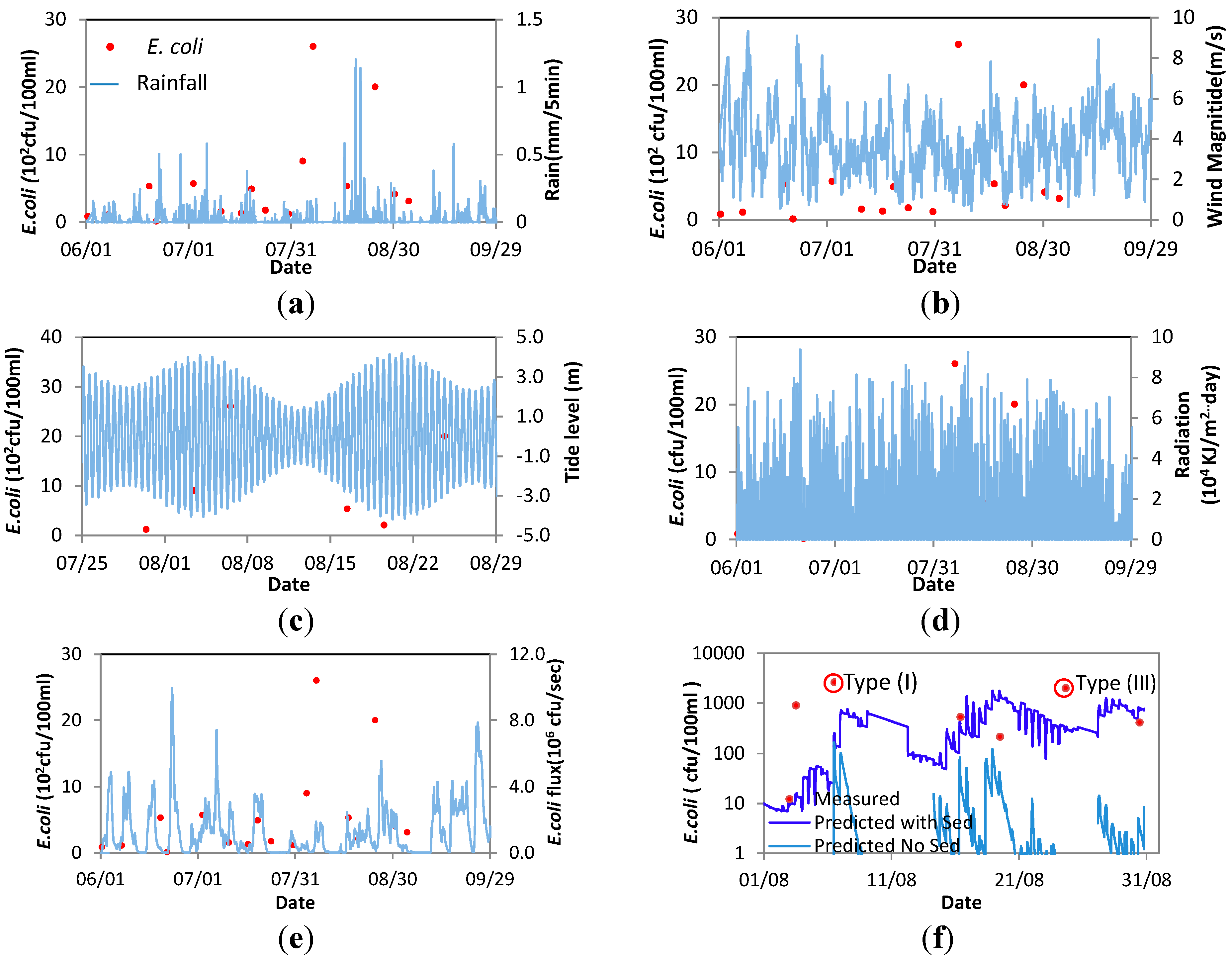
4.2. Factors Influencing the High FIO Concentration Events at Bathing Sites in 2012

The key factors influencing a high E. coli concentration event for a bathing site can be investigated by comparing the antecedent riverine inputs and the prevailing weather, hydrological, tidal, water quality conditions, and the temporal and spatial processes governing the E. coli concentrations in the river and coastal regions using the 2D model. Firstly, E. coli concentration data, sampled during the period from May to September in 2012, at 29 bathing water regions (BWR) in the study site (see Figure 1) were acquired, together with the associated spatially averaged rainfall and solar radiation levels for the sub-catchments, and wind and tidal levels near the 29 bathing sites. All of these data were acquired at 15 min intervals (see Figure 6a–d). Secondly, the process representation for each of these factors may influence the high E. coli concentration levels in the BWR, with E. coli fluxes predicted for the river and BWRs being shown in Figure 6e. Thirdly, the E. coli concentration levels, obtained with and without sediment coupling are shown in Figure 6f, which can be used to better understand the impact of sediment coupling on the E. coli levels at the bathing water sites.

Figure 6. Example site (No. 41800) for recognising event types at bathing water site (See Figure 1 for location) (a) E. coli and Rainfall; (b) E. coli and wind magnitude; (c) E. coli and tidal level process; (d) E. coli and riverine Radiation; (e) E. coli and riverine E. coli flux input; (f) E. coli calculated with and without sediment coupling.

Figure 6. Example site (No. 41800) for recognising event types at bathing water site (See Figure 1 for location) (a) E. coli and Rainfall; (b) E. coli and wind magnitude; (c) E. coli and tidal level process; (d) E. coli and riverine Radiation; (e) E. coli and riverine E. coli flux input; (f) E. coli calculated with and without sediment coupling.

From the data provided in the six individual graphs shown in Figure 6, the episodic high FIO concentration events, and the related driving factors at the bathing sites near Southport, the Flyde Coast and Blackpool, are analysed and listed in Table 3. In Table 3, HC indicates that the E. coli concentration is higher than the good quality level and LC indicates it is lower than the level required for the EU Bathing Water Directives. The good standards for E. coli in 1976 and 2006 Bathing Water Directives are 1000 cfu/100 mL and 500 cfu/100 mL, respectively.

Based on the findings in Table 3, four main types of high concentration events are identified as follows:

(I) Intense rainfall linked events. Among the 20 high E. coli concentration events, about 8 of these events are caused by large storms, with intense rainfall-runoff rates, especially for small catchments. The overflows from CSOs and sewage water storage under such storm conditions also contribute to the higher FIO concentrations.

(II) Accumulated and first wash-off events. If the weather conditions are moderate and suitable for FIOs to survive for several days in the catchments and river bed, ponds and sewage tanks, for example, then for a moderate rainfall event, enough soil moisture, lower solar radiation and continuous sediment deposition can lead to the accumulated FIOs in the catchments and rivers arriving at the coastal receiving waters with a high concentration. For such a condition, even moderate rainfall can result in high FIO concentrations, e.g., up to 3000~4000 cfu/100 mL. Of the 20 events considered, there are about 4 events which fit this category.

(III) Delivery and resuspension events. This is usually caused by large E. coli fluxes inflowing from the main rivers, but can also be generated by spring tides. Some E. coli can survive in the attached sediment particles for more than 2 months [82] and can then be transported to the BWRs by the advection or re-suspension of fine sediments, under the action of tidal currents and strong wind induced waves. For example, E. coli from the main rivers, including the Ribble, Mersey and Leven, may arrive at the BWRs having been transported via the sediments for some distance from the corresponding river estuaries. Therefore, these rivers may have a more permanent influence on the bathing water quality than intense rainfall events. Usually, this kind of event is regarded as secondary and the peak concentration is less than 2000 cfu/100 mL.

(IV) Mixed events. Such events include more than two of the event types mentioned above. Generally speaking, the peak concentrations are larger than the individual event types and they have a more comprehensive influence on the E. coli levels at the bathing water sites. For example, E. coli concentration levels of 6500 and 7000 cfu/100 mL arrived at bathing sites 42,100 and 42,300 on 24 June 2012, respectively, driven by continuous rainfall, strong winds and possibly local sewage emissions on 22 June 2012. These inputs had a wide impact on the bathing sites to the north, at 42,500, 42,600 and 42,800 (see Table 3).

Table 3. High E. coli concentration events and the key identified impact factors at 11 bathing water compliance sites (see Figure 1 for locations).

BWR No.	1976/EC	2006/EC	Peak and Time (cfu/100 mL)	Key Driving Factor	Event Type
41200	LC	HC	827 (17 August)	Rainfall and Ribble flux	& (III)
41300	HC	HC	1100 (25 June)	Rainfall and Ribble flux	(I) & (III)
41500	HC	HC	1300 (25 June)	Rainfall and Ribble flux	(I) & (III)
	LC	HC	750 (5 August)	Local rain or transport	(I) and (II)
41800	HC	HC	2600 (6 August)	Antecedent dry weather before	(II)
	HC	HC	2000 (24 August)	Local large rainfall	& (III)
41900	HC	HC	4800 (6 August)	Antecedent dry weather before	(II)
	HC	HC	2000 (24 August)	Local large rainfall	(I)
42100	HC	HC	6500 (24 June)	Rainfall and Wind	(IV)
	HC	HC	2600 (28 August)	Local large rainfall	(III)
42300	HC	HC	7000 (24 June)	rainfall and strong Wind	(IV)
	HC	HC	1900 (28 August)	Local middle rainfall	(III)
42500	HC	HC	5000 (24 June)	Intense rainfall and strong Wind	(IV)
	HC	HC	1100 (28 August)	Ribble middle rainfall	(III)
42600	HC	HC	4600 (24 June)	Intense rainfall and strong Wind	(III) & (I)
	LC	HC	900 (28 August)	Ribble middle rainfall	(III)
42800	HC	HC	4800 (24 June)	Intense rainfall and strong Wind	(III) & (I)
	HC	HC	3200 (6 August)	Small radiation	(III)
43000	HC	HC	3200 (6 August)	High tide	(III)
	HC	HC	1400 (16 August)	Local middle rainfall	(I)

Table 3. High E. coli concentration events and the key identified impact factors at 11 bathing water compliance sites (see Figure 1 for locations).

BWR No.	1976/EC	2006/EC	Peak and Time (cfu/100 mL)	Key Driving Factor	Event Type
41200	LC	HC	827 (17 August)	Rainfall and Ribble flux	& (III)
41300	HC	HC	1100 (25 June)	Rainfall and Ribble flux	(I) & (III)
41500	HC	HC	1300 (25 June)	Rainfall and Ribble flux	(I) & (III)
	LC	HC	750 (5 August)	Local rain or transport	(I) and (II)
41800	HC	HC	2600 (6 August)	Antecedent dry weather before	(II)
	HC	HC	2000 (24 August)	Local large rainfall	& (III)
41900	HC	HC	4800 (6 August)	Antecedent dry weather before	(II)
	HC	HC	2000 (24 August)	Local large rainfall	(I)
42100	HC	HC	6500 (24 June)	Rainfall and Wind	(IV)
	HC	HC	2600 (28 August)	Local large rainfall	(III)
42300	HC	HC	7000 (24 June)	rainfall and strong Wind	(IV)
	HC	HC	1900 (28 August)	Local middle rainfall	(III)
42500	HC	HC	5000 (24 June)	Intense rainfall and strong Wind	(IV)
	HC	HC	1100 (28 August)	Ribble middle rainfall	(III)
42600	HC	HC	4600 (24 June)	Intense rainfall and strong Wind	(III) & (I)
	LC	HC	900 (28 August)	Ribble middle rainfall	(III)
42800	HC	HC	4800 (24 June)	Intense rainfall and strong Wind	(III) & (I)
	HC	HC	3200 (6 August)	Small radiation	(III)
43000	HC	HC	3200 (6 August)	High tide	(III)
	HC	HC	1400 (16 August)	Local middle rainfall	(I)

Based on the data given in Table 3, it can be seen that there are 5 and 11 BWRs, out of 11, where the BWRs could not meet the minimum mandatory EC 1976 and 2006 standards, respectively. Therefore, further catchment clean-up operations and an integrated river and beach management strategy could be desirable in order to achieve a higher level of bathing water status in the future. Different methods may be adopted for high concentration events, including: (1) reducing direct inputs of raw sewage by additional infrastructure and enhancing the treatment standard for waste water could be considered in addressing type (I) and (II) events; (2) modifying any near-shore outfall locations away from the bathing sites could be a more efficient way of improving bathing water quality; and (3) improving catchment management by increasing plant quarantine zones and fencing off rivers, thereby improving livestock grazing and manure modes, and constructing ecological purification ponds may assist in controlling FIO input levels from diffuse sources. In addition, this study shows that an integrated modelling system is an effective tool for assessing the impact of various alternative options to improve bathing water quality.

5. Conclusions

An integrated modelling system for predicting the hydrologic, hydrodynamic, sediment and E. coli transport and decay processes from source regions in catchments to coastal receiving waters has been developed by linking a grid based distributed hydrological model, a one-dimensional river networks model and a modified EFDC-2D model. The integrated model is capable of predicting the E. coli concentration distributions in the source regions and their impact on the receiving bathing waters. The model has been applied to a large and complex water system, which includes 11 river catchments and the associated estuaries. An extensive data set, including meteorologic, hydrologic and hydrodynamic data, and information concerning soil and sediment types, land use and livestock density was considered in supporting the modelling and bathing water management plans. The model was verified against appropriate data and the model results generally fit well with the measured data, although further refinement of the sediment adsorption and desorption parameters for E. coli could be studied further to improve the model accuracy.

It has been established that the model predicted sediment yield, transport, erosion and deposition vary significantly for the different types of catchments. More research is needed to investigate the mechanisms of sediment yield and transport in these catchments. The integrated model is currently used to identify the main factors and event types for high FIO concentration events in the BWRs. The goal is to quantitatively evaluate the response of the bathing water quality for different types of BWRs and for a variety of clean-up management options, for various meteorological, hydrological and tidal hydrodynamic conditions.

Finally, the model predictions have shown then when sediment transport is included as a key transport mechanism for FIOs in the river basin and coastal receiving waters, then improved predictions are obtained when the measured and predicted E. coli levels are compared. Hence, this study shows that it is desirable to include sediment transport processes and the adsorption or desorption of E. coli to or from the sediments when investigating bathing water quality. If sediment transport fluxes of FIOs are not included in river basin modelling, then concentration levels predicted in the coastal receiving waters may be lower than expected for the modelled meterologic, hydrologic and hydrodynamic conditions considered.

References

1. Kay, D.; Edwards, A.C.; Ferrier, R.; Francis, C.; Kay, C.; Rushby, L.; Watkins, J.; McDonald, A.T.; Wyer, M.; Crowther, J. Catchment Microbial Dynamics: The Emergence of a Research Agenda. Prog. Phys. Geogr. 2007, 31, 59–76. [Google Scholar]
2. Figueras, M.; Borrego, J.J. New perspectives in monitoring drinking water microbial quality. Int. J. Environ. Res. Public Health 2010, 7, 4179–4202. [Google Scholar]
3. European Environment Agency (EEA). European Bathing Water Quality in 2013; European Environment Agency (EEA) Report No 1/2014; EEA: Copenhagen, Denmark, 2014; pp. 1–32. [Google Scholar]
4. Pompepuy, M.; Catherine, M.; Le Saux, J.C.; Joanny, M.; Camus, P. Impacts of Microbiological Contamination on the Marine Environment of the North-East Atlantic; OSPAR Commission: London, UK, 2009; pp. 1–23. [Google Scholar]
5. European Union (EU). Directive 2006/7/EC of the European Parliament and of the Council of 15 February 2006 Concerning the Management of Bathing Water Quality and Repealing Directive 76/160/EE. Available online: http://eur-lex.europa.eu/legal-content/EN/TXT/?uri=celex:32006L0007 (accessed on 31 August 2015).
6. Stapleton, C.M.; Wyer, M.D.; Crowther, J.; McDonald, A.T.; Kay, D.; Greaves, J.; Wither, A.; Watkins, J.; Francis, C.; Humphrey, N.; et al. Quantitative catchment profiling to apportion faecal indicator organism budgets for the Ribble system, the UK’s sentinel drainage basin for Water Framework Directive research. J. Environ. Manag. 2008, 87, 535–550. [Google Scholar]
7. Kay, D.; Crowther, J.; Stapleton, C.M.; Wyer, M.D.; Fewtrell, L.; Anthony, S.; Bradford, M.; Edwards, A.; Francis, C.A.; Hopkins, M.; et al. Faecal indicator organism concentrations and catchment export coefficients in the UK. Water Res. 2008, 42, 2649–2661. [Google Scholar]
8. Lin, B.; Syed, M.; Falconer, R.A. Predicting faecal indicator levels in estuarine receiving waters—An integrated hydrodynamic and ANN modelling approach. Environ. Model. Softw. 2008, 23, 729–740. [Google Scholar]
9. Kashefipour, S.M.; Lin, B.; Falconer, R.A. Modelling the fate of faecal indicators in a coastal basin. Water Res. 2006, 40, 1413–1425. [Google Scholar] [CrossRef] [PubMed]
10. De Brauwere, A.; Gourgue, O.; de Brye, B.; Servais, P.; Ouattara, N.K.; Deleersnijder, E. Integrated modelling of faecal contamination in a densely populated river–sea continuum (Scheldt River and Estuary). Sci. Total Environ. 2014, 468–469, 31–45. [Google Scholar] [CrossRef] [PubMed]
11. Tetzlaff, D.; Capell, R.; Soulsby, C. Land use and hydroclimatic influences on Faecal Indicator Organisms in two large Scottish catchments: Towards land use-based models as screening tools. Sci. Total Environ. 2012, 434, 110–122. [Google Scholar]
12. Solvi, A.-M. Modelling the Sewer-Treatment-Urban River System in View of the EU Water Framework Directive. Ph.D. Thesis, Ghent University, Ghent, Belgium, 2007. [Google Scholar]
13. Benham, B.; Baffaut, C.; Zeckoski, R.; Mankin, K.; Pachepsky, Y.; Sadeghi, A.; Brannan, K.; Soupir, M.; Habersack, M. Modeling bacteria fate and transport in watersheds to support TMDLs. Trans. ASAE 2006, 49, 987–1002. [Google Scholar]
14. Crane, B.S.; Moore, J. Modeling enteric bacterial die-off: A review. Water Air Soil Pollut. 1986, 27, 411–439. [Google Scholar]
15. Medema, G.; Bahar, M.; Schets, F. Survival of Cryptosporidium parvum, Escherichia coli, faecal enterococci and Clostridium perfringens in river water: Influence of temperature and autochthonous microorganisms. Water Sci. Technol. 1997, 35, 249–252. [Google Scholar]
16. Thupaki, P.; Phanikumar, M.S.; Schwab, D.J.; Nevers, M.B.; Whitman, R.L. Evaluating the role of sediment-bacteria interactions on Escherichia coli concentrations at beaches in southern Lake Michigan. J. Geophys. Res.: Oceans 2013, 118, 7049–7065. [Google Scholar]
17. Gao, G.; Falconer, R.A.; Lin, B. Modelling importance of sediment effects on fate and transport of enterococci in the Severn Estuary, UK. Mar. Pollut. Bull. 2013, 67, 45–54. [Google Scholar]
18. Bai, S.; Lung, W.-S. Modeling Sediment Impact on the Transport of Fecal Bacteria. Water Res. 2005, 39, 5232–5240. [Google Scholar]
19. American Society of Agricultural Engineers (ASAE). American Society of Agricultural Engineers (ASAE) Standards D384.1: Manure Production and Characteristics; ASAE: St Joseph, MI, USA, 1998. [Google Scholar]
20. Coffey, R.; Cummins, E.; Bhreathnach, N.; Flaherty, V.O.; Cormican, M. Development of a pathogen transport model for Irish catchments using SWAT. Agric. Water Manag. 2010, 97, 101–111. [Google Scholar]
21. USEPA. Bacterial Indicator Tool User’s Guide; EPA-832-B-01-003; USEPA: Washington, DC, USA, 2000.
22. Zeckoski, R.; Benham, B.; Shah, S.; Wolfe, M.; Brannan, K.; Al-Smadi, M.; Dillaha, T.; Mostaghimi, S.; Heatwole, C. BSLC: A tool for bacteria source characterization for watershed management. Appl. Eng. Agric. 2005, 21, 879–892. [Google Scholar]
23. Faust, M.A. Relationship between land-use practices and fecal bacteria in soils. J. Environ. Qual. 1982, 11, 141–146. [Google Scholar]
24. Hutchison, M.; Walters, L.; Moore, A.; Crookes, K.; Avery, S. Effect of length of time before incorporation on survival of pathogenic bacteria present in livestock wastes applied to agricultural soil. Appl. Environ. Microbiol. 2004, 70, 5111–5118. [Google Scholar]
25. Vadas, P.; Kleinman, P.; Sharpley, A. A simple method to predict dissolved phosphorus in runoff from surface-applied manures. J. Environ. Qual. 2004, 33, 749–756. [Google Scholar]
26. Chick, H. An investigation of the laws of disinfection. J. Hyg. 1908, 8, 92–158. [Google Scholar]
27. Brookes, J.D.; Antenucci, J.; Hipsey, M.; Burch, M.D.; Ashbolt, N.J.; Ferguson, C. Fate and transport of pathogens in lakes and reservoirs. Environ. Int. 2004, 30, 741–759. [Google Scholar]
28. Cho, K.H.; Pachepsky, Y.A.; Kim, J.H.; Kim, J.-W.; Park, M.-H. The modified SWAT model for predicting fecal coliforms in the Wachusett Reservoir Watershed, USA. Water Res. 2012, 46, 4750–4760. [Google Scholar]
29. Reddy, K.; Khaleel, R.; Overcash, M. Behavior and transport of microbial pathogens and indicator organisms in soils treated with organic wastes. J. Environ. Qual. 1981, 10, 255–266. [Google Scholar]
30. Gerba, C.P.; Melnick, J.L.; Wallis, C. Fate of wastewater bacteria and viruses in soil. J. Irrig. Drain. Div. 1975, 101, 157–174. [Google Scholar]
31. Tian, Y.Q.; Gong, P.; Radke, J.D.; Scarborough, J. Spatial and temporal modeling of microbial contaminants on grazing farmlands. J. Environ. Qual. 2002, 31, 860–869. [Google Scholar]
32. Nagels, J.; Davies-Colley, R.; Donnison, A.; Muirhead, R. Faecal contamination over flood events in a pastoral agricultural stream in New Zealand. Water Sci. Technol. 2002, 45, 45–52. [Google Scholar]
33. Muirhead, R.W.; Davies-Colley, R.J.; Donnison, A.M.; Nagels, J.W. Faecal bacteria yields in artificial flood events: Quantifying in-stream stores. Water Res. 2004, 38, 1215–1224. [Google Scholar]
34. Wheeler Alm, E.; Burke, J.; Spain, A. Fecal indicator bacteria are abundant in wet sand at freshwater beaches. 2003, 37, 3978–3982. [Google Scholar] [CrossRef]
35. Passerat, J.; Ouattara, N.K.; Mouchel, J.-M.; Vincent, R.; Servais, P. Impact of an intense combined sewer overflow event on the microbiological water quality of the Seine River. Water Res. 2011, 45, 893–903. [Google Scholar]
36. Even, S.; Mouchel, J.-M.; Servais, P.; Flipo, N.; Poulin, M.; Blanc, S.; Chabanel, M.; Paffoni, C. Modelling the impacts of Combined Sewer Overflows on the river Seine water quality. Sci. Total Environ. 2007, 375, 140–151. [Google Scholar]
37. Chapra, S. Surface Water-Quality Modeling; WCB McGraw-Hill: Boston, MA, USA, 1997. [Google Scholar]
38. Ling, T.; Achberger, E.; Drapcho, C.; Bengtson, R. Quantifying adsorption of an indicator bacteria in a soil-water system. Trans. Asae 2002, 45, 669–674. [Google Scholar]
39. Chin, D.; Sakura-Lemessy, D.; Bosch, D.; Gay, P. Watershed-scale fate and transport of bacteria. Trans. ASABE 2009, 52, 145–154. [Google Scholar]
40. Kay, D.; Wyer, M.; Crowther, J.; Stapleton, C.; Bradford, M.; McDonald, A.; Greaves, J.; Francis, C.; Watkins, J. Predicting faecal indicator fluxes using digital land use data in the UK’s sentinel Water Framework Directive catchment: The Ribble study. Water Res. 2005, 39, 3967–3981. [Google Scholar]
41. Servais, P.; Garcia-Armisen, T.; George, I.; Billen, G. Fecal bacteria in the rivers of the Seine drainage network (France): Sources, fate and modelling. Sci. Total Environ. 2007, 375, 152–167. [Google Scholar]
42. Borah, D.; Bera, M. Watershed-scale hydrologic and nonpoint-source pollution models: Review of mathematical bases. Trans. ASAE 2003, 46, 1553–1566. [Google Scholar]
43. Papanicolaou, A.; Bdour, A.; Wicklein, E. One-dimensional hydrodynamic sediment transport model applicable to steep mountain streams. J. Hydraul. Res. 2004, 42, 357–375. [Google Scholar]
44. Papanicolaou, A.N.; Sanford, J.T.; Dermisis, D.C.; Mancilla, G.A. A 1-D Morphodynamic Model for Rill Erosion. Water Resour. Res. 2010, 46. [Google Scholar] [CrossRef]
45. Liang, D.; Lin, B.; Falconer, R.A. Simulation of rapidly varying flow using an efficient TVD-MacCormack scheme. Int. J. Numer. Methods Fluids 2007, 53, 811–826. [Google Scholar]
46. Garcia-Navarro, P.; Alcrudo, F.; Saviron, J. 1-D open-channel flow simulation using TVD-McCormack scheme. J. Hydraul. Eng. 1992, 118, 1359–1372. [Google Scholar]
47. Ji, Z. General hydrodynamic model for sewer/channel network systems. J. Hydraul. Eng. 1998, 124, 307–315. [Google Scholar]
48. Garcia-Navarro, P.; Alcrudo, F.; Priestley, A. An implicit method for water flow modelling in channels and pipes. J. Hydraul. Res. 1994, 32, 721–742. [Google Scholar]
49. Djordjevic, S.; Prodanovic, D.; Walters, G.A. Simulation of transcritical flow in pipe/channel networks. J. Hydraul. Eng. 2004, 130, 1167–1178. [Google Scholar]
50. Kashefipour, S.M.; Lin, B.; Harris, E.; Falconer, R.A. Hydro-Environmental Modelling for Bathing Water Compliance of an Estuarine Basin. Water Res. 2002, 36, 1854–1868. [Google Scholar]
51. De Brauwere, A.; de Brye, B.; Servais, P.; Passerat, J.; Deleersnijder, E. Modelling Escherichia coli concentrations in the tidal Scheldt river and estuary. Water Res. 2011, 45, 2724–2738. [Google Scholar] [CrossRef] [PubMed]
52. Bedri, Z.; Corkery, A.; O’Sullivan, J.J.; Alvarez, M.X.; Erichsen, A.C.; Deering, L.A.; Demeter, K.; O’Hare, G.M.; Meijer, W.G.; Masterson, B. An integrated catchment-coastal modelling system for real-time water quality forecasts. Environ. Model. Softw. 2014, 61, 458–476. [Google Scholar]
53. Shrestha, N.K.; Leta, O.T.; de Fraine, B.; van Griensven, A.; Bauwens, W. OpenMI-based integrated sediment transport modelling of the river Zenne, Belgium. Environ. Model. Softw. 2013, 47, 193–206. [Google Scholar]
54. Amaguchi, H.; Kawamura, A.; Olsson, J.; Takasaki, T. Development and testing of a distributed urban storm runoff event model with a vector-based catchment delineation. J. Hydrol. 2012, 420–421, 205–215. [Google Scholar] [CrossRef]
55. Zhao, R. The Xinanjiang model applied in China. J. Hydrol. 1992, 135, 371–381. [Google Scholar]
56. Lu, M.; Li, X. Time scale dependent sensitivities of the XinAnJiang model parameters. Hydrol. Res. Lett. 2014, 8, 51–56. [Google Scholar]
57. O’Callaghan, J.F.; Mark, D.M. The extraction of drainage networks from digital elevation data. Comput. Visi. Graph. Image Process. 1984, 28, 323–344. [Google Scholar]
58. Alam, M.J.; Dutta, D. A process-based and distributed model for nutrient dynamics in river basin: Development, testing and applications. Ecol. Model. 2012, 247, 112–124. [Google Scholar]
59. Wu, W. Computational River Dynamics; CRC Press: Boca Raton, FL, USA, 2008. [Google Scholar]
60. Jamieson, R.; Gordon, R.; Joy, D.; Lee, H. Assessing microbial pollution of rural surface waters: A review of current watershed scale modeling approaches. Agric. Water Manag. 2004, 70, 1–17. [Google Scholar]
61. Pachepsky, Y.A.; Sadeghi, A.; Bradford, S.; Shelton, D.; Guber, A.; Dao, T. Transport and fate of manure-borne pathogens: Modeling perspective. Agric. Water Manag. 2006, 86, 81–92. [Google Scholar]
62. Meselhe, E.A.; Holly, F.M., Jr. Simulation of Unsteady Flow in Irrigation Canals with Dry Bed. J. Hydraul. Eng. 1993, 119, 1021–1039. [Google Scholar]
63. Hamrick, J.M. A Three-Dimensional Environmental Fluid Dynamics Computer Code: Theoretical and Computational Aspects; Virginia Institute of Marine Science, College of William and Mary: Gloucester Point, VA, USA, 1992. [Google Scholar]
64. Huang, G.; Falconer, R.A.; Boye, B.A.; Lin, B. Cloud to coast: Integrated assessment of environmental exposure, health impacts and risk perceptions of faecal organisms in coastal waters. Int. J. River Basin Manag. 2015, 13, 73–86. [Google Scholar]
65. Nachtergaele, F.; van Velthuizen, H.; Verelst, L.; Batjes, N.; Dijkshoorn, K.; van Engelen, V.; Fischer, G.; Jones, A.; Montanarella, L.; Petri, M. Harmonized World Soil Database; Food and Agriculture Organization of the United Nations: Rome, Italy, 2008. [Google Scholar]
66. The British Atmospheric Date Centre. Available online: http://badc.nerc.ac.uk/home/ (accessed on 31 August 2015).
67. Center for Ecology and Hydrology. Available online: http://www.ceh.ac.uk/data/nrfa/data/search.html (accessed on 31 August 2015).
68. Morris, D.; Flavin, R. Sub-set of the UK 50 m by 50 m Hydrological Digital Terrain Model Grids; NERC, Institute of Hydrology: Wallingford, UK, 1994. [Google Scholar]
69. Moore, R.; Morris, D.; Flavin, R. Sub-set of UK Digital 1: 50,000 Scale River Centre-Line Network; NERC, Institute of Hydrology: Wallingford, UK, 1994. [Google Scholar]
70. British Geological Survey. Available online: http://www.bgs.ac.uk/products/offshore/DigSBS250.html (accessed on 31 August 2015).
71. Pye, K.; Blott, S.J.; Witton, S.J.; Pye, A.L. Cell 11 Regional Monitoring Strategy Results of Sediment Particle Size Analysis; Report (Kenneth Pye Associates Ltd.); Kenneth Pye Associates Ltd.: Solihull, UK, 2010; p. 1. [Google Scholar]
72. Digimap Home Page. Available online: http://digimap.edina.ac.uk/digimap/home (accessed on 31 August 2015).
73. Weather and Climate Met Office. Available online: http://www.metoffice.gov.uk/ (accessed on 31 August 2015).
74. Office for National Statistics. Available online: http://www.ons.gov.uk/ons/index.html (accessed on 31 August 2015).
75. Welcome to GOV.UK. Available online: https://www.gov.uk (accessed on 31 August 2015).
76. Bathing Water Quality. Available online: http://environment.data.gov.uk/bwq/profiles/ (accessed on 31 August 2015).
77. Frey, S.K.; Topp, E.; Edge, T.; Fall, C.; Gannon, V.; Jokinen, C.; Marti, R.; Neumann, N.; Ruecker, N.; Wilkes, G.; Lapen, D.R. Using SWAT, Bacteroidales microbial source tracking markers, and fecal indicator bacteria to predict waterborne pathogen occurrence in an agricultural watershed. Water Res. 2013, 47, 6326–6337. [Google Scholar]
78. Kim, J.-W.; Pachepsky, Y.A.; Shelton, D.R.; Coppock, C. Effect of streambed bacteria release on E. coli concentrations: Monitoring and modeling with the modified SWAT. Ecol. Model. 2010, 221, 1592–1604. [Google Scholar]
79. Ouattara, N.K.; de Brauwere, A.; Billen, G.; Servais, P. Modelling faecal contamination in the Scheldt drainage network. J. Mar. Syst. 2013, 128, 77–88. [Google Scholar]
80. Whitman, R.L.; Nevers, M.B. Summer E. coli patterns and responses along 23 Chicago beaches. Environ. Sci. Technol. 2008, 42, 9217–9224. [Google Scholar]
81. De Marchis, M.; Freni, G.; Napoli, E. Modelling of E. coli distribution in coastal areas subjected to combined sewer overflows. Water Sci. Technol. 2013, 68, 1123–1136. [Google Scholar] [CrossRef] [PubMed] [Green Version]
82. Davies, C.M.; Long, J.; Donald, M.; Ashbolt, N.J. Survival of fecal microorganisms in marine and freshwater sediments. Appl. Environ. Microbiol. 1995, 61, 1888–1896. [Google Scholar] [PubMed]