Simulation of Water Level Fluctuations in a Hydraulic System Using a Coupled Liquid-Gas Model

Abstract

A model for simulating vertical water level fluctuations with coupled liquid and gas phases is presented. The Preissmann implicit scheme is used to linearize the governing equations for one-dimensional transient flow for both liquid and gas phases, and the linear system is solved using the chasing method. Some classical cases for single liquid and gas phase transients in pipelines and networks are studied to verify that the proposed methods are accurate and reliable. The implicit scheme is extended using a dynamic mesh to simulate the water level fluctuations in a U-tube and an open surge tank without consideration of the gas phase. Methods of coupling liquid and gas phases are presented and used for studying the transient process and interaction between the phases, for gas phase limited in a chamber and gas phase transported in a pipeline. In particular, two other simplified models, one neglecting the effect of the gas phase on the liquid phase and the other one coupling the liquid and gas phases asynchronously, are proposed. The numerical results indicate that the asynchronous model performs better, and are finally applied to a hydropower station with surge tanks and air shafts to simulate the water level fluctuations and air speed.

1. Introduction

Transient effects often occur in pipelines and networks of pipelines, both when transporting liquid and gas. For pipelines transporting liquids, most studies found in the literature focus on the water hammer effect that is caused by inappropriate operation. The water hammer effect may damage the pipeline or other equipment. For pipelines transporting gas, research has instead focused on the transportation capacity and on-line control. For instance, customer demand imposes dynamic conditions for pipelines transporting natural gas. Further, an efficient gas network is important due to the length of the pipelines, which may be hundreds of kilometers.

One-dimensional (1D) methods for transient flow analysis satisfy most engineering application requirements. Compared with 2D and 3D methods, 1D methods have the advantages of high speed computation and easy boundary condition implementation, especially when the pipeline system is very long or complex. The disadvantage of 1D methods is that they cannot simulate flow such as complex two-phase flow, vortex flow and present detailed flow information. The governing equations for 1D transient flow are the continuity equation and the momentum equation. These form a pair of nonlinear hyperbolic partial differential equations. The flow in both the gas phase and liquid phase are governed by the same equations. The same numerical techniques are thus suitable for pipelines transporting both liquid and gas. The existing popular 1D numerical methods include the method of characteristics (MOC), the finite difference method (FD), the finite volume method (FV).

MOC, as proposed by Chaudhry [1] and Wylie and Streeter [2], is widely used in engineering practice because of the simplicity in coding and the high efficiency in computation ([3,4]). The partial differential equations are transformed along characteristics lines, and grid nodes are not always present on these characteristics lines for fixed grids. Two issues are particularly important when programming: (1) the time steps must correlate with the space steps because of the Courant-Friedrichs-Lewy (CFL) limitation and (2) interpolation or wave speed adjustment must be implemented when using fixed grids. Much work has been done to further advance the MOC. For instance, linear ([5,6,7,8,9,10]) and nonlinear ([11]) interpolation methods have been implemented in space or time. Rohani and Afshar [12] proposed a point-implicit method of characteristics (PIMOC) to calculate the transient flow caused by the closure of a valve and the failure of a pump system. They found that the PIMOC required less computational effort compared with the original implicit method of characteristics ([13]) due to the reduced size of the nonlinear system of equations while yielding the same results. FD methods are also widely used in numerical simulations. Different FD schemes can be distinguished by the order of precision or space formats, and the relationship between different time steps. Chaudhry and Hussaini [14] solved the water hammer equations through the explicit FD method using the MacCormak, Lambda, and Gabutti schemes, and found that for the same accuracy, these second-order schemes require fewer computational nodes and less computer time compared to conventional MOC. Jin et al. [15] used a spatial four-point implicit FD method to solve the unsteady flow processes of a drainage system and found that the method exhibited good stability and a wide application scope. Pezzinga [16] proposed a quasi-2D mathematical model with an implicit FD scheme for unsteady turbulent flow in pipes and pipe networks, and concluded that a quasi-2D model can improve the prediction of high-frequency transients compared with a 1D model.

FV methods can also be used for water hammer simulations. Guinot [17], Hwang and Chung [18], Zhao and Ghidaoui [19], León et al. [20], and Sabbagh-Yazdi et al. [21] formulated first- and second-order explicit FV methods of the Godunov type for solving water hammer problems. All these studies concluded that second-order Godunov-type methods are more accurate and faster.

The governing equations for water hammer and gas flow have a very similar format. Therefore, the same numerical methods (including the methods mentioned above) are appropriate both for pipelines transporting both liquid or gas. Greyvenstein [22] and Pretoriu et al. [23] simulated flow in pipe networks for both gas and liquid phases with the same method. Wylie and Streeter [24], Chaudhry [1] and Osiadacz [25] used MOC to simulate gas flows. Kessal [26] and Thorley and Tiley [27] used FD methods. Ibraheem and Adewumi [28], Zhou and Adewumi [29], Einfeldt [30] simulated transients in gas pipelines using FV methods. Herrán-González et al. [31], Behbahani-Nejad and Bagheri [32] and Alamian [33] proposed gas transient flow simulations based on the state space equations, solved using a MATLAB-Simulink transfer function. Ke and Ti [34] extended an electrical analogy method to transient analysis of isothermal gas flows in a pipeline network.

Pipelines with single-phase liquid or gas flow can be simulated using the water hammer equations and the gas flow equations, respectively. However, in some cases, liquid and gas phases coexist in the same pipeline. For instance, the drop shaft in a sewer system is always characterized by a mixture of air and water, and the air phase has a great influence on the capacity of the drop shaft and hydraulic pressure [35]. Also, in underground hydroelectric stations, the surge tank always connects to the outside air tunnels, thus at the water level a liquid–gas interface is present. The two phases influence each other during transient processes and high velocity gas flows may appear in the air tunnels because the area of the surge tank is far larger than that of the air duct. In this application, the liquid–gas interface is always horizontal and single, so that a general two-phase flow model is not necessary for simulation and a simple model can instead be utilized.

The purpose of this work is to couple the liquid and gas flow transient governing equations in order to simulate the water level fluctuation in vertical ducts, to determine the time-varying parameters such as water level, pressure, and flow discharge. To achieve this objective, the Preissmann four-point implicit scheme is applied to some classical examples in order to verify the accuracy of the method in liquid and gas pipeline flow. Next, the water hammer equations are extended to calculate water-level fluctuations in open-type surge tanks and U-tubes by the implicit dynamic mesh method. The water level in an air cushion surge chamber is then simulated by coupling the water hammer equations and the ideal gas state equation. A model with coupled 1D liquid and gas pipeline flow is then proposed to understand the interaction of the two phases. Two other simplified approaches—one neglecting the effect of the gas phase on the liquid phase and one coupling the liquid and gas phases asynchronously—are presented and verified by examples. Finally, this coupling method is applied to a hydropower project under construction with a large area surge tank attached to the pipeline transporting gas.

2. Governing Equations and Numerical Methods

2.1. 1D Water Hammer Equations

The governing equations for 1D unsteady flow of a compressible liquid in an elastic pipeline are the continuity and momentum equations, given by

$$V\frac{\partial H}{\partial x}+\frac{\partial H}{\partial t}+\frac{a^2}{g}\frac{\partial V}{\partial x}+\frac{a^{2}V}{gA}\frac{\partial A}{\partial x}-\sin \text{β}\cdot V=0$$

(1)

$$g\frac{\partial H}{\partial x}+V\frac{\partial V}{\partial x}+\frac{\partial V}{\partial t}+f\frac{V\left|V\right|}{2D}=0$$

(2)

here, x and t are space and time coordinates, respectively; V is the mean flow velocity in the pipe; H is the piezometri head; a is the speed of sound; A is the cross-sectional area of the pipe; β is the pipe slope; g is the gravitational acceleration; f is the Darcy-Weisbach friction factor, which is a function of velocity [36], but it is considered as a constant because of the slight influence on transient flow; and D is the inner diameter of the pipe.

2.2. 1D Governing Equations for Gas Flow

The governing equations for gas flow are the continuity and momentum equations, given by

$$\frac{B^2}{A}\frac{\partial M}{\partial x}+\frac{\partial p}{\partial t}=0$$

(3)

$$\frac{\partial p}{\partial x}+\frac{\text{1}}{A}\frac{\partial M}{\partial t}+\frac{pg}{B^2}\sin \text{β}+\frac{f{B}^2{M}^2}{2D{A}^{2}p}=0$$

(4)

where x and t are space and time coordinates; M is the mass flow rate; p is the absolute pressure; B is the acoustic wave speed; A is the cross-sectional area of the pipe; β is the pipe slope; g is the gravitational acceleration; f is the Darcy-Weisbach friction factor; and D is the inner diameter of the pipe.

2.3. Solution of the Governing Equations

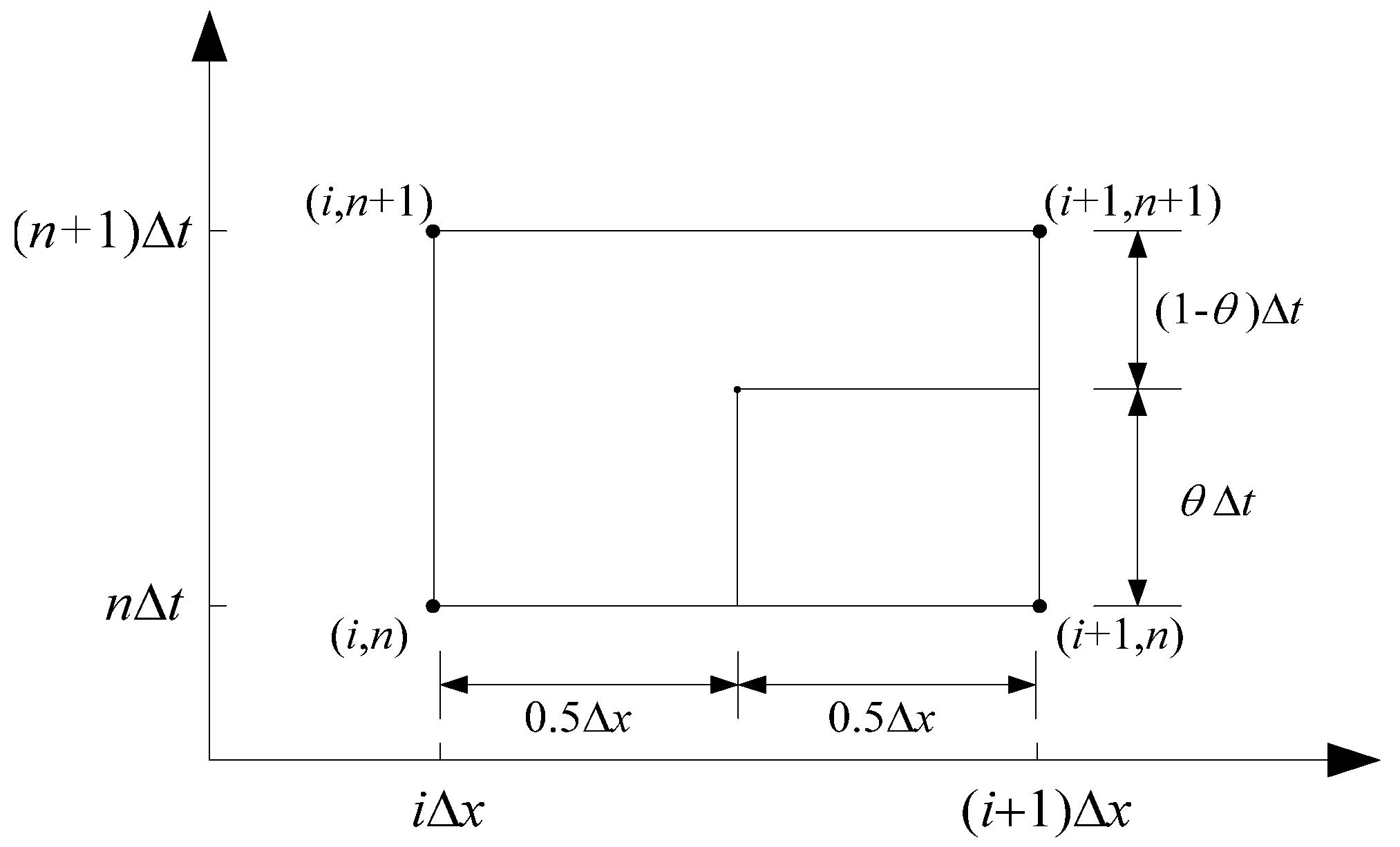
2.3.1. Finite Difference Scheme

The Preissmann space four-point implicit finite difference scheme with one weight coefficient is given by

$$\begin{array}{l}f(x,t)=\frac{\text{θ}}{2}\left(f_{i+1}^{n+1}+f_i^{n+1}\right)+\frac{1-\text{θ}}{2}\left(f_{i+1}^n+f_i^n\right)\\ \frac{\partial f}{\partial x}=\text{θ}\frac{f_{i+1}^{n+1}-f_i^{n+1}}{\text{Δ}x}+\left(1-\text{θ}\right)\frac{f_{i+1}^n-f_i^n}{\text{Δ}x}\\ \frac{\partial f}{\partial t}=\frac{f_{i+1}^{n+1}-f_{i+1}^n+f_i^{n+1}-f_i^n}{2\text{Δ}t}\end{array}$$

(5)

here, f (x,t) denotes the value of $f_i^n$ at the point(x,t) = (iΔx, nΔt); i and n indicate space and time directions, respectively; and θ is the weight coefficient. Figure 1 shows a graphical interpretation of the scheme. Using the discharge, Q, instead of the velocity, V in the liquid phase water hammer Equations (1) and (2), the discrete equations expressed in incremental form can be written as

$$A1\times \text{Δ}{H}_{i+1}+B1\times \text{Δ}{Q}_{i+1}\text{=\hspace{0.05em}}C1\times \text{Δ}{H}_i+D1\times \text{Δ}{Q}_i+F1$$

(6)

$$A2\times \text{Δ}{H}_{i+1}+B2\times \text{Δ}{Q}_{i+1}\text{=}C2\times \text{Δ}{H}_i+D2\times \text{Δ}{Q}_i+F2$$

(7)

here, subscript i is the node number; and ΔH and ΔQ are the time step increments in pressure head and discharge, respectively. Parameters A1(A2), B1(B2), C1(C2), D1(D2), F1(F2) are known values related to the duct area, the mesh size, the time step, and flow at the last time step. Expressions for these parameters can be found in Appendix A. The discrete equations for the gas phase, Equations (3) and (4), can in the same way be written in incremental form as

$$A1\times \text{Δ}{p}_{i+1}+B1\times \text{Δ}{M}_{i+1}\text{=\hspace{0.05em}}C1\times \text{Δ}{p}_i+D1\times \text{Δ}{M}_i+F1$$

(8)

$$A2\times \text{Δ}{p}_{i+1}+B2\times \text{Δ}{M}_{i+1}\text{=}C2\times \text{Δ}{p}_i+D2\times \text{Δ}{M}_i+F2$$

(9)

here, Δp and ΔM are the increments of pressure and mass flow rate, respectively, in the gas phase, Expressions for these parameters can be found in Appendix A.

Figure 1. Graphical view of the numerical scheme of the Preissmann method.

Figure 1. Graphical view of the numerical scheme of the Preissmann method.

2.3.2. Solution Method

We use the liquid phase as an example to explain how one applies the chasing method to solve the linear matrix equations. The chasing method includes forward and backward scans in two main steps. Equations (6) and (7) are written for every node, i. For a pipeline of N computational nodes (N−1 computational grids), there are only 2N−2 discretized equations but 2N unknowns. Therefore, inlet and outlet boundary conditions are needed to close the system. Transforming the inlet boundary condition f(Q₁, H₁) = 0.0 to an incremental representation results in the establishment of a relationship between the pressure head and the discharge, as

$$\text{Δ}{Q}_1=E{E}_1\times \text{Δ}{H}_1+F{F}_1$$

(10)

Coefficients EE₁ and FF₁ are known from the linearization. Substituting Equation (10) into Equations (6) and (7) and applying recursion relations between pressure head and discharge of every node, i.e., the forward scan process, yields:

$$\text{Δ}{Q}_i=E{E}_i\times \text{Δ}{H}_i+F{F}_i$$

(11)

$$\text{Δ}{H}_i=L_i\times \text{Δ}{H}_{i+1}+M_i\times \text{Δ}{Q}_{i+1}+N_i$$

(12)

here, EE_i and FF_i are known coefficients resulting from the recursion and are related to EE_i−1, FF_i−1. The relational expression at the last node can be obtained by the forward scan process, as

$$\text{Δ}{Q}_N=E{E}_N\times \text{Δ}{H}_N+F{F}_N$$

(13)

The unknown parameters ∆Q_N and ∆H_N are obtained by combining the outlet boundary condition f(Q_N, H_N) = 0.0 and Equation (13). ∆H_N−1 can be solved by Equation (12), then ∆Q_N−1 can be obtained by Equation (11). All unknown values can be obtained by the recursion relations Equations (11) and (12), which are known as the backward scan process. Linearization and all coefficients for Equations (10)–(13) are presented in reference [37].

3. Verification of the Scheme

Three validation cases are here used to show that the Preissmann implicit scheme is valid and accurate for both liquid flow and gas flow, both in single pipelines and in networks of pipelines. The validation provides the basis for coupling the liquid and gas phase in the next sections.

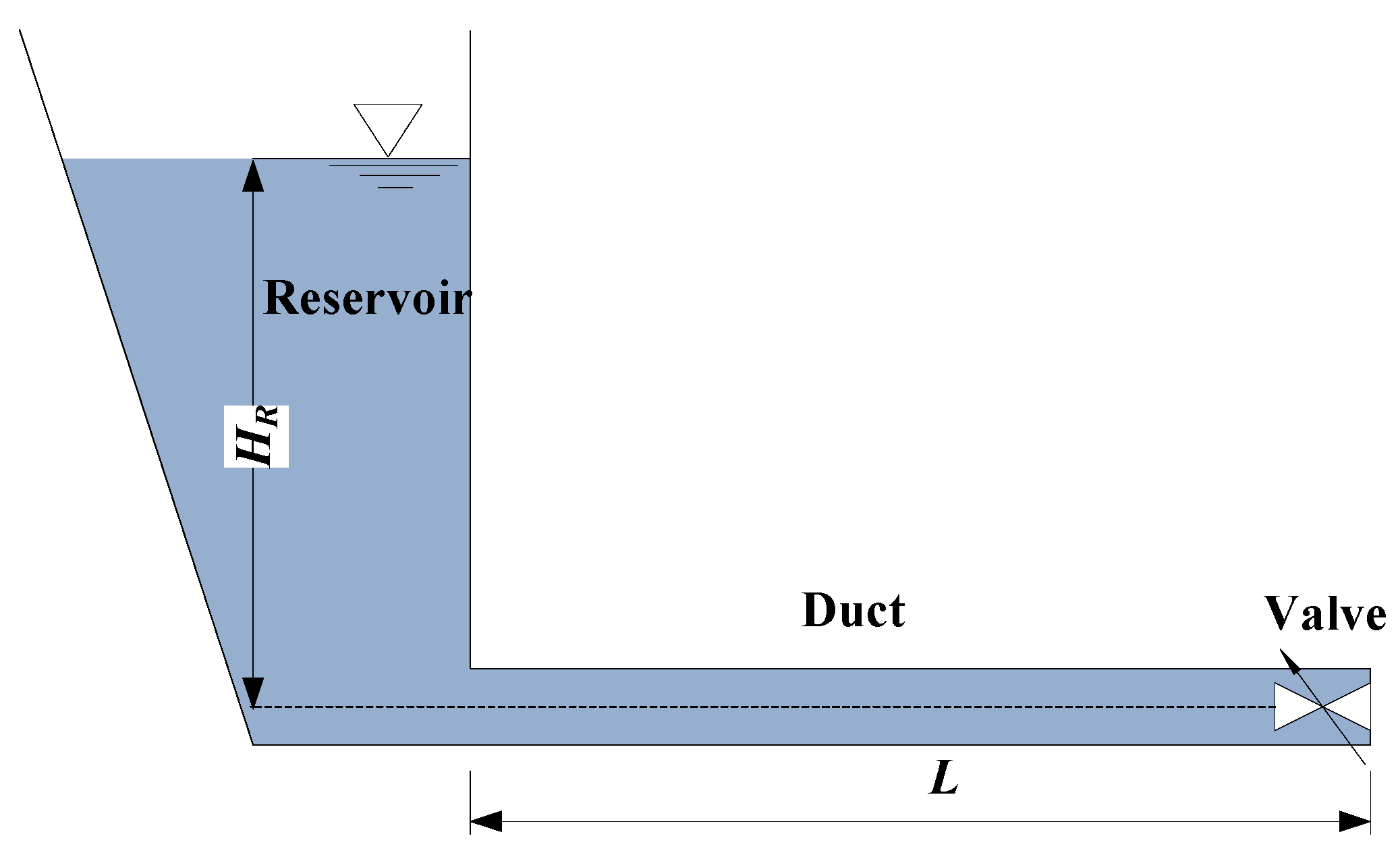
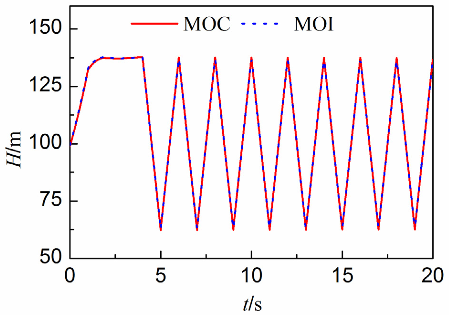
3.1. Verification of the Liquid Phase

A reservoir-pipe-valve system, such as that shown in Figure 2, is used to validate the implicit FD scheme for modeling a water hammer wave under three conditions. The pipe is 500 m long and 4 m² in cross-sectional area, and the friction factor is 0.014. The initial discharge is 10 m³/s and the reservoir head and valve closing time are varied in each condition according to:

• Case 1: Infinite reservoir with a steady head of 100 m, with the valve closed suddenly;
• Case 2: Infinite reservoir with a steady head of 100 m, with the valve closed linearly over 4 s;
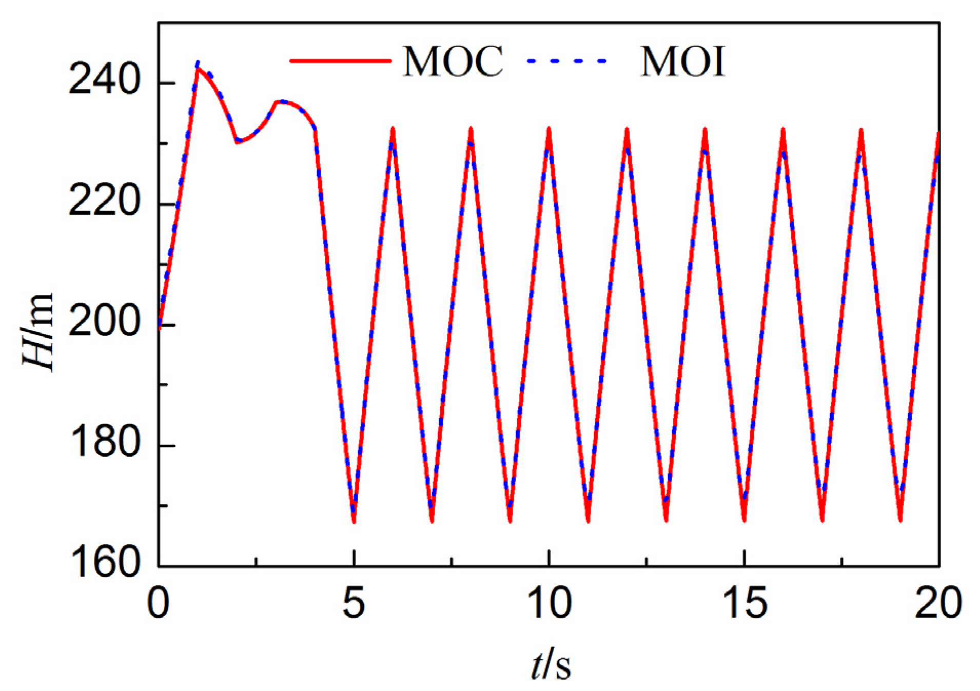
• Case 3: Infinite reservoir with a steady head of 200 m, with the valve closed linearly over 4 s.

Figure 2. A reservoir-pipe-valve system.

Figure 2. A reservoir-pipe-valve system.

Figure 3, Figure 4 and Figure 5 compare the pressure head at the valve between the MOC and the methods of implicit (MOI) Preissmann scheme presented above. Both the extreme value and the period of the water hammer waves in the three cases as calculated by MOI agree well with those calculated by MOC, and the relative error is less than 5%, which implies that the Preissmann implicit scheme is valid for simulating liquid transient flow in pipelines.

Figure 3. Pressure head traces at the valve for Case 1.

Figure 3. Pressure head traces at the valve for Case 1.

Figure 4. Pressure head traces at the valve for Case 2.

Figure 4. Pressure head traces at the valve for Case 2.

Figure 5. Pressure head traces at the valve for Case 3.

Figure 5. Pressure head traces at the valve for Case 3.

3.2. Verification of the Gas Phase

3.2.1. A Single Straight Gas Pipe

This test case is the single horizontal straight gas pipe used by Herrán-González [31]. The specified periodic demand at the outlet is shown in Figure 6. The boundary condition at the pipe inlet is a constant pressure of 50 bars. The duct is 100 km in length and 0.6 m in diameter with a friction factor of 0.012 (equal to 0.003 in reference [31] because the friction term is expressed by fB²M²/2DA²p here rather than 2fB²M²/2DA²p by Herrán-González). The operating temperature is 278 K, the gas constant is 392 m²·s⁻²·K⁻¹, and the gas density is 0.73 kg/m³. The initial pressure distribution and sound speed are determined for steady state conditions as

$$p_l^2=(p_0^2-\frac{f{B}^2{M}^2}{D{A}^2}\text{Δ}x\frac{e^s-1}{s})/e^s$$

(14)

$$B^2=CRT$$

(15)

$$C=1-\frac{p_{\text{0}}+p_l}{390\times 2}$$

(16)

here, s = (2gΔxsinβ)/B²; C is the compressibility factor; R is the gas constant and T is the absolute temperature. At x = 0, p = p₀, at x = ∆x, p = p_l. The time step is 0.05 s and 100 nodes are used for the discretization. Figure 7 shows the obtained outlet pressure fluctuation trace by the MOI scheme as compared with the result calculated by Herrán-González [31], which has a similar behavior and the relative error does not exceed 5%.

Figure 6. Gas demand at the outlet.

Figure 6. Gas demand at the outlet.

Figure 7. Pressure traces at the outlet.

Figure 7. Pressure traces at the outlet.

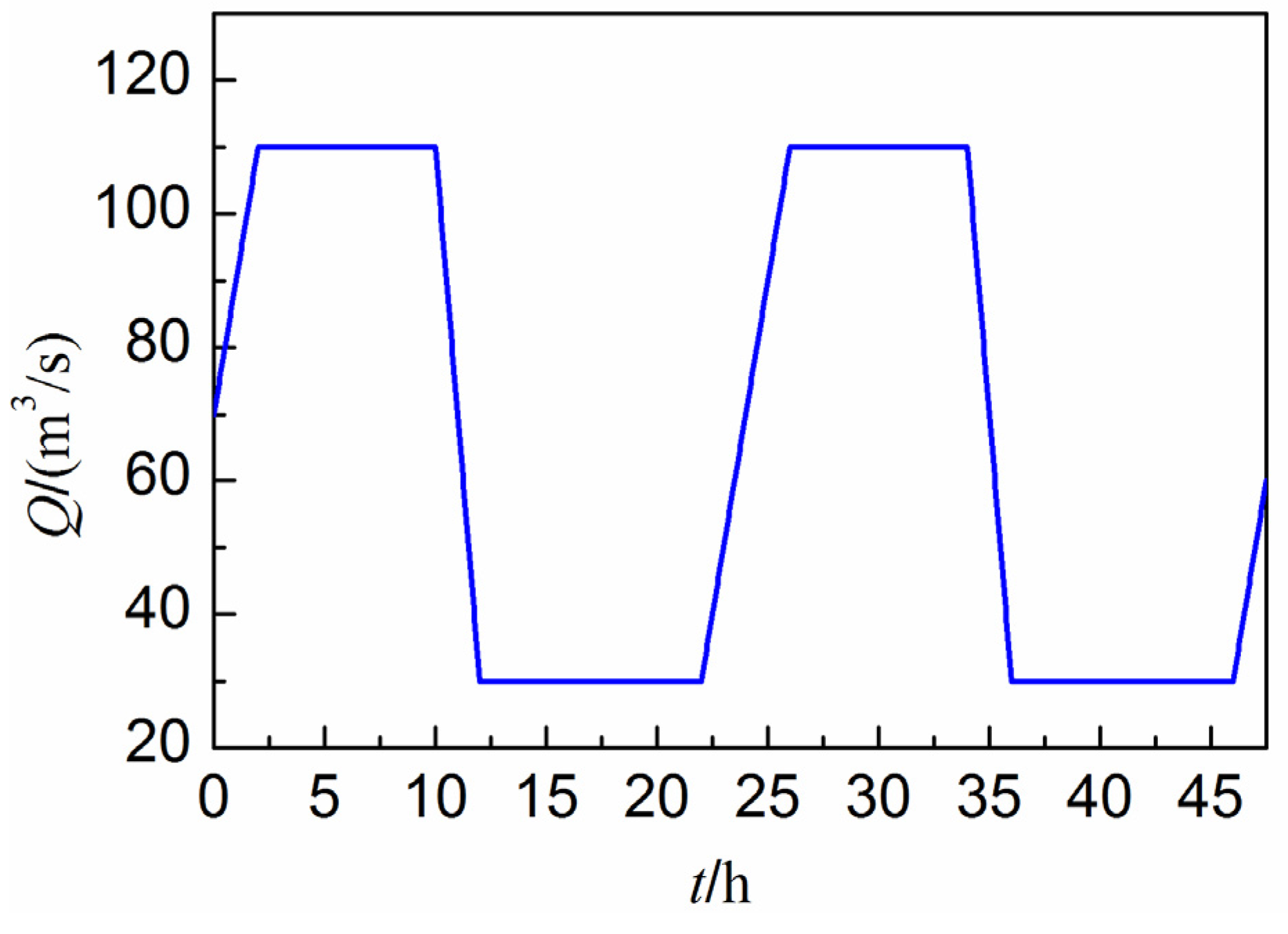
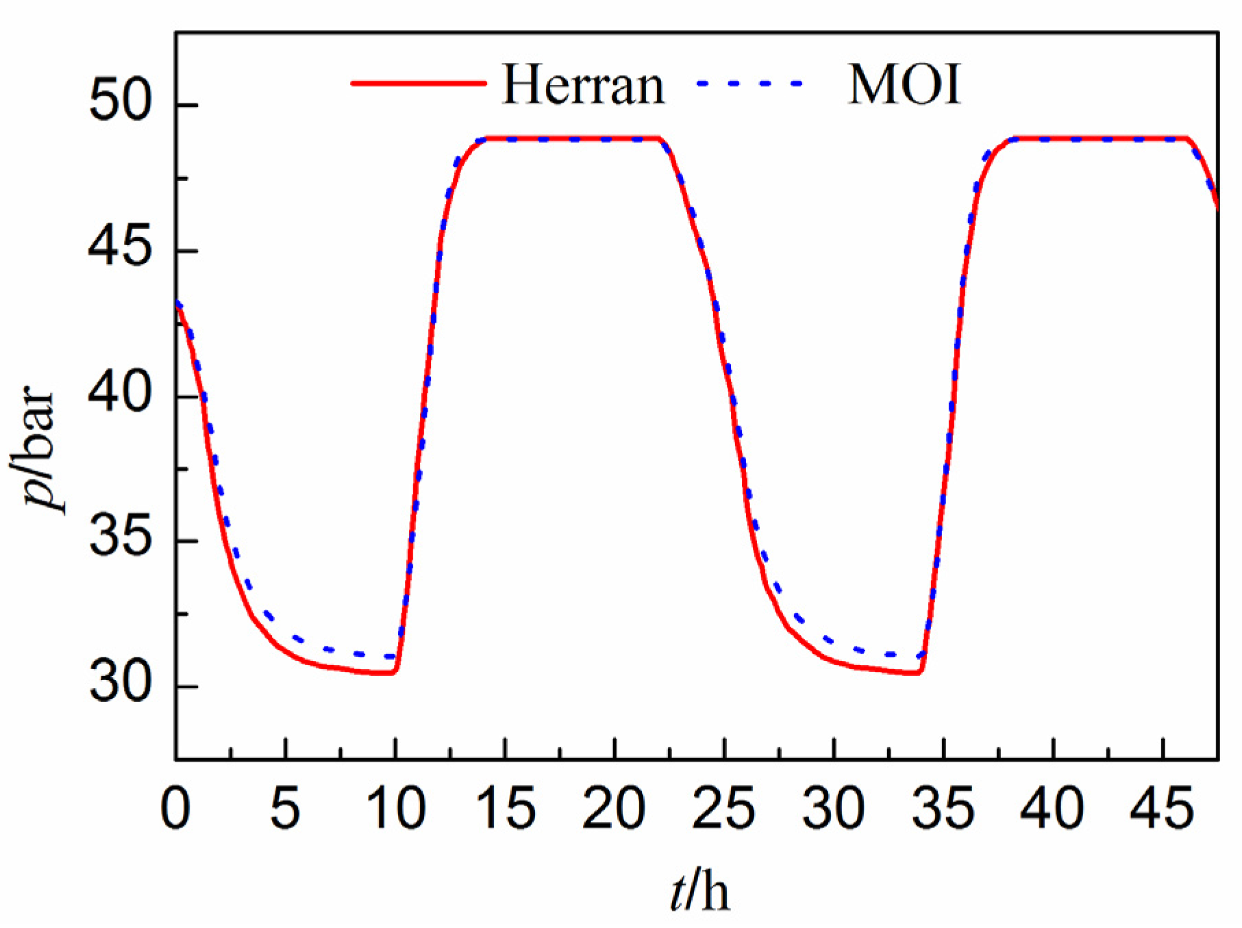
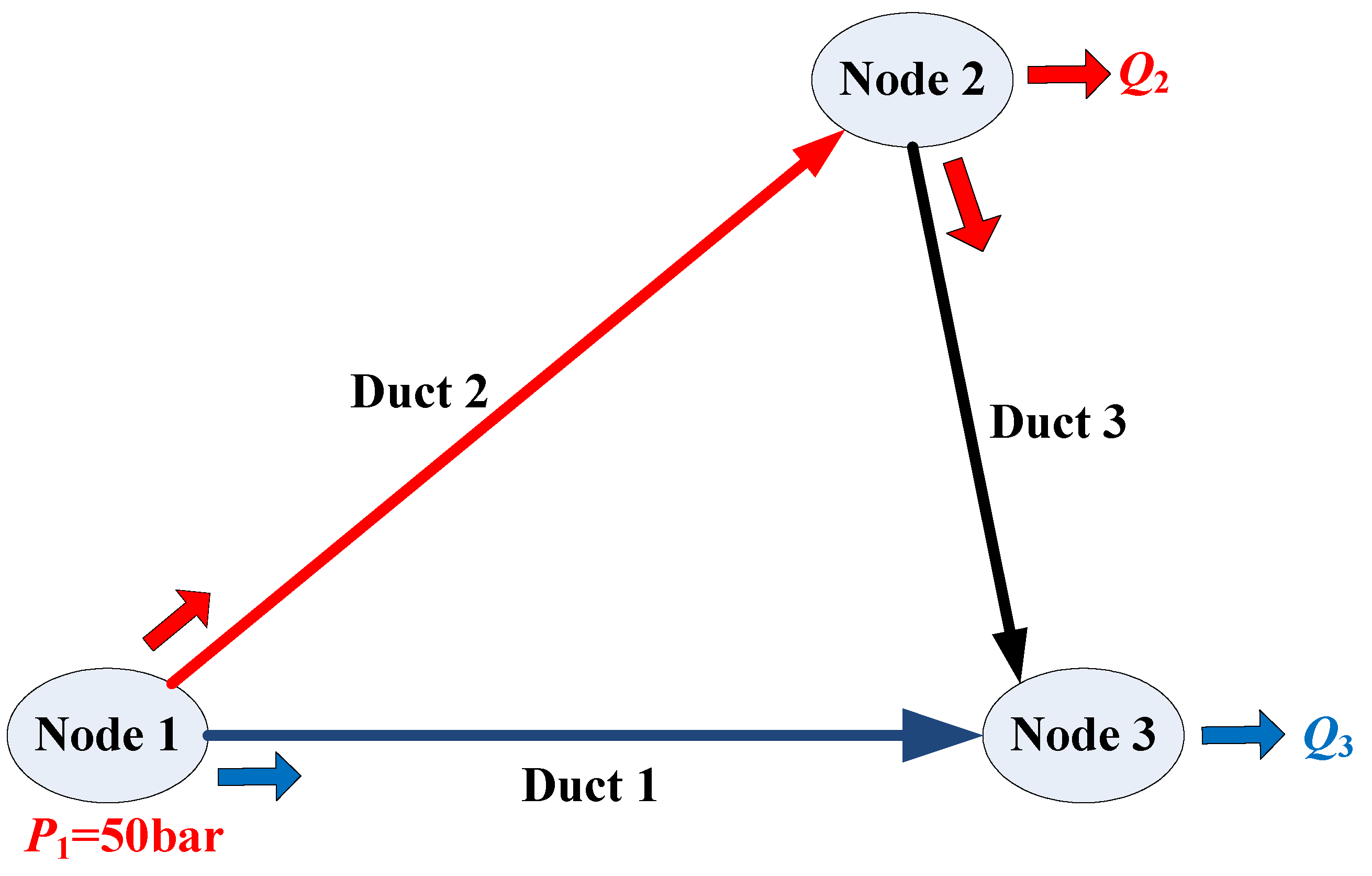
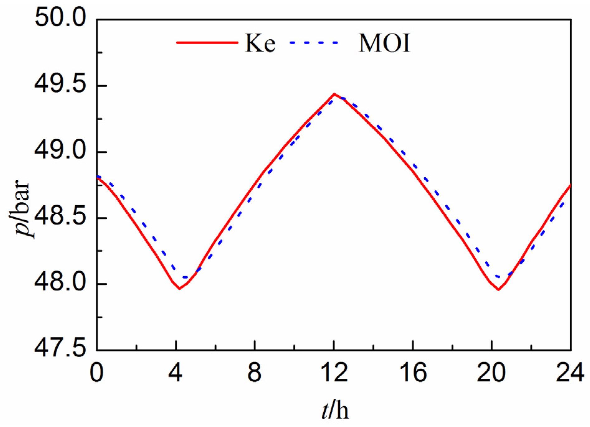
3.2.2. A Gas Pipeline Network

Figure 8 shows a gas pipeline network composed of three horizontal ducts. The length of Duct 1, Duct 2, and Duct 3 are 80 km, 90 km, and 100 km, respectively. The diameter of all three ducts is 0.6 m. Node 1 is the pressure inlet with a constant pressure of 50 bars, which supplies the gas flow for the network. Node 2 and Node 3 are discharge outlets and the gas demand over time is shown in Figure 9. The gas density is 0.7165 kg/m³ with a specific gravity of 0.6, and the friction factor is 0.012. The operating temperature is 278 K and the gas constant is 392 m²·s⁻²·K⁻¹. The initial pressure field is determined by Equations (14)–(16). The calculation time step is 0.05 s and each duct is divided into 100 numerical nodes. Figure 10 and Figure 11 show the transient changes in pressure at Node 2 and Node 3 compared with the results presented by Ke and Ti [34], and the relative error does not exceed 5% between the two methods. The results show that the MOI is valid for modeling the gas flow in the network.

Figure 8. Schematic diagram of gas networks.

Figure 8. Schematic diagram of gas networks.

Figure 9. Gas demand at Nodes 2 and 3.

Figure 9. Gas demand at Nodes 2 and 3.

Figure 10. Pressure traces at Node 2.

Figure 10. Pressure traces at Node 2.

Figure 11. Pressure traces at Node 3.

Figure 11. Pressure traces at Node 3.

4. Simulation of Water Level Fluctuations

Most problems related to water level fluctuations involve the coupling between liquid and gas phases. The present work relates to transient processes in hydropower stations, where water level fluctuation phenomena exist in surge tanks. The phenomena can be divided into three categories. The first category ignores the effect of the gas phase, such as water level fluctuations in an open surge tank or a U-tube. The water surface then reaches the atmosphere directly and the interface pressure remains constant during the wave processes. The second category involves the approximation that the gas phase is limited to a chamber. The pressure of the gas thus varies with the water level, since the gas volume is determined by the water level. Under such conditions, the two phases interact and the gas phase is described by the ideal gas state equations. The third category refers to the situation in which the gas phase exists in pipelines and the flow behavior can be described by the continuity and momentum equations, as shown in Equations (3) and (4). The pressure at the interface is often determined by the geometry of the gas ducts, such as its cross-sectional area and length. The water level fluctuation can only be clearly influenced by the gas phase if the pressure at the interface significantly changes, since liquids are far denser than gases. Such a situation can be found in underground hydropower stations, where the surge tank links to the outside atmosphere by gas pipelines. The cross-sectional area of the surge tank is far greater than that for the gas ducts, so the water level fluctuations in the tank may lead to high wind speed in the gas ducts.

4.1. Neglecting the Influence of the Gas Phase

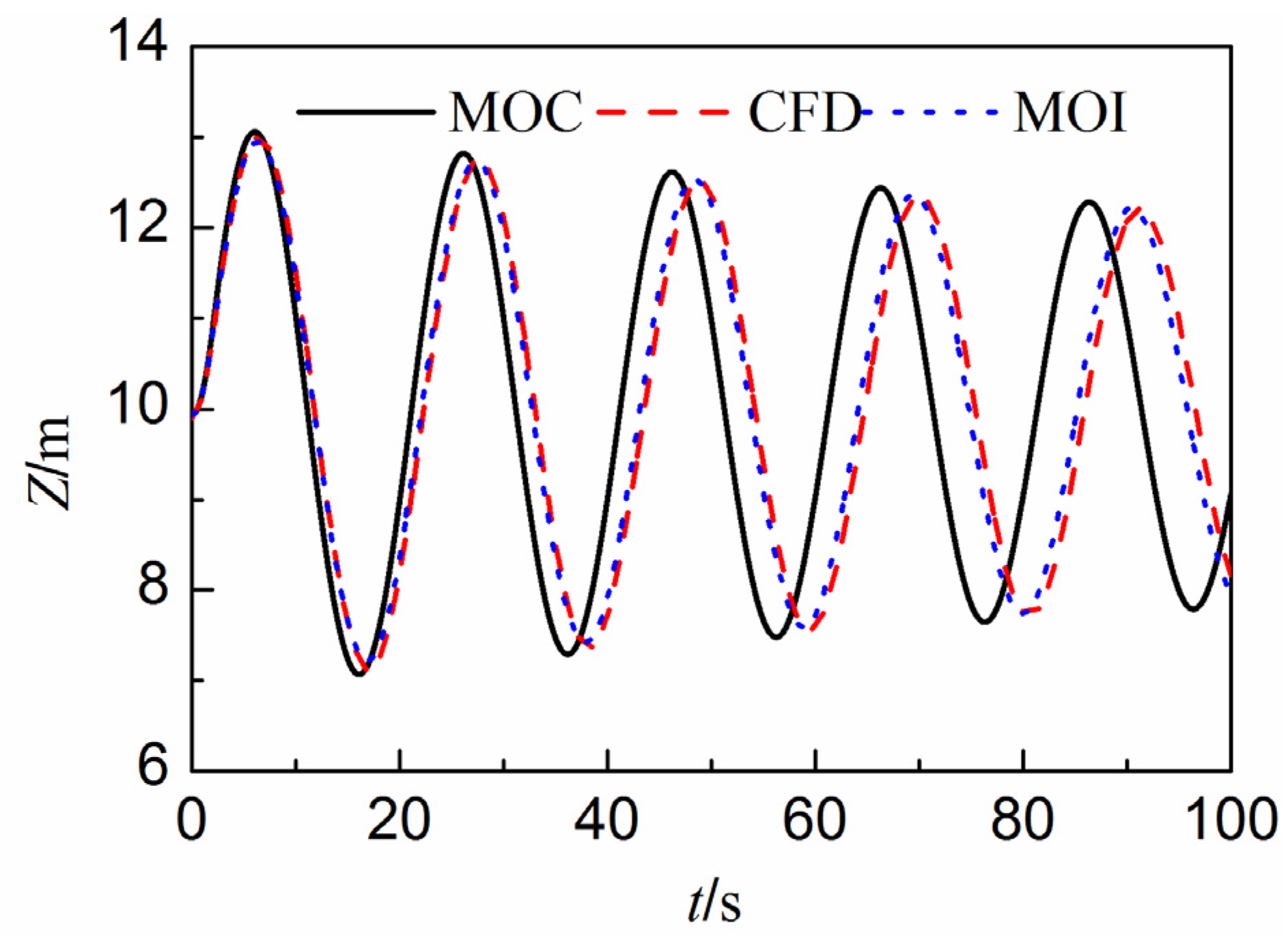
4.1.1. Water Level Fluctuations in an Open Surge Tank

The open surge tank, as shown in Figure 12, is an important hydraulic structure in hydropower stations. Accurate surge calculations determine the size of the surge tank and influence other regulative and protective parameters during the design process. Many numerical methods have been proposed to simulate water level fluctuations. The most popular approach is to couple MOC with the boundary conditions of the surge tank. This neglects the inertial forces and the frictional losses in the tank, and assumes a hydrostatic pressure variation. However, this method is invalid or inaccurate for small surge tanks because the vertical velocity changes may be significant.

Figure 12. Reservoir-surge tank-valve system.

Figure 12. Reservoir-surge tank-valve system.

The Volume of Fluid (VOF) model used in Computational Fluid Dynamics (CFD) can also be used to simulate the fluctuating water level in surge tanks, and is considered to be one of the most accurate methods for tracking interfaces. However, CFD is not efficient for hydropower stations with diversion tunnels that are dozens of kilometers long.

A method is here proposed to simulate water level fluctuations by extending the use of the water hammer equations. As shown in Figure 13, the surge tank is treated as a pipeline. The discharge and the pressure head field are solved using MOI, using a dynamic mesh to track the surface. The liquid phase above the maximum mesh is assumed to be a hydrostatic pressure variation, which does not take into account inertial forces and frictional losses. The algorithm of the method is shown from Step 1 to Step 6.

Figure 13. Computational grid for the surge tank.

Figure 13. Computational grid for the surge tank.

Step 1: Obtain EE₁ and FF₁

$$Q_{sn}=Q_{CP}-C_{QP}\cdot H_{sn}$$

(17)

$$Q_{x1}=Q_{CM}+C_{QM}\cdot H_{x1}$$

(18)

$$Q_{sn}=Q_1+Q_{x1}$$

(19)

$$H_{sn}=H_{x1}=H_1+\alpha Q_1^2$$

(20)

Step 2: Process of forward scan to get EE_i and FF_i

$$\text{Δ}{Q}_i=E{E}_i\times \text{Δ}{H}_i+F{F}_i$$

(21)

$$\text{Δ}{H}_i=L_i\times \text{Δ}{H}_{i+1}+M_i\times \text{Δ}{Q}_{i+1}+N_i$$

(22)

Step 3: Solve for pressure head, discharge of Node N and water level

$$Z\text{=}{Z}^{\text{0}}\text{+(}{Q}_N\text{+}{Q}_N^0\text{)Δ}t\text{/2}F$$

(23)

$$Q_N-Q_N^0=E{E}_N\times \text{(}{H}_N-H_N^0\text{)}+F{F}_N$$

(24)

$$H_N=Z$$

(25)

Step 4: Process of backward scan

for i = N − 1, …, 0 do

$$\text{Δ}{H}_i=L_i\times \text{Δ}{H}_{i+1}+M_i\times \text{Δ}{Q}_{i+1}+N_i$$

(26)

$$\text{Δ}{Q}_i=E{E}_i\times \text{Δ}{H}_i+F{F}_i$$

(27)

end for

Step 5: Adjust the mesh for next time step

$$\frac{Z}{\text{Δ}x}-1\le N\text{-}new<\frac{Z}{\text{Δ}x}$$

(28)

Step 6: Initialization for next time step

$$Z^{\text{0}}=Z$$

(29)

for i = 0,…, N−new do

$$Q_i^0\text{=}{Q}_i$$

(30)

$$H_i^0\text{=}{H}_i$$

(31)

end for

if (N−new > N)

$$Q_{N\text{-}new}^0\text{=}{Q}_N$$

(32)

$$H_{N\text{-}new}^0\text{=}Z$$

(33)

end if

In Equations (17)–(33), Q and H are the discharge and pressure head, respectively; subscript i is the mesh node number as shown in Figure 13; superscript 0 signifies a parameter at the previous time step and new predicates the current time step; Q_CP (C_QP, Q_CM, and C_QM) is the MOC coefficient [24] for the pipelines in front and behind the surge tank; EE_i (FF_i, L_i, M_i, N_i) is the coefficient in Equations (10)–(13); α is the discharge coefficient of the orifice; and ∆x is the mesh size; F and Z are the cross-section area and water level of the surge tank, respectively.

Consider the reservoir-surge tank valve system shown in Figure 12. The lengths of Duct 1 and Duct 2 are 100 m and 50 m, respectively, and the cross sectional areas of the two ducts and the surge tank are 1 m². The friction factor is 0.014 and the initial steady discharge of the valve is 1 m³/s. The MOI, as here proposed, is compared with MOC and CFD in the following two cases.

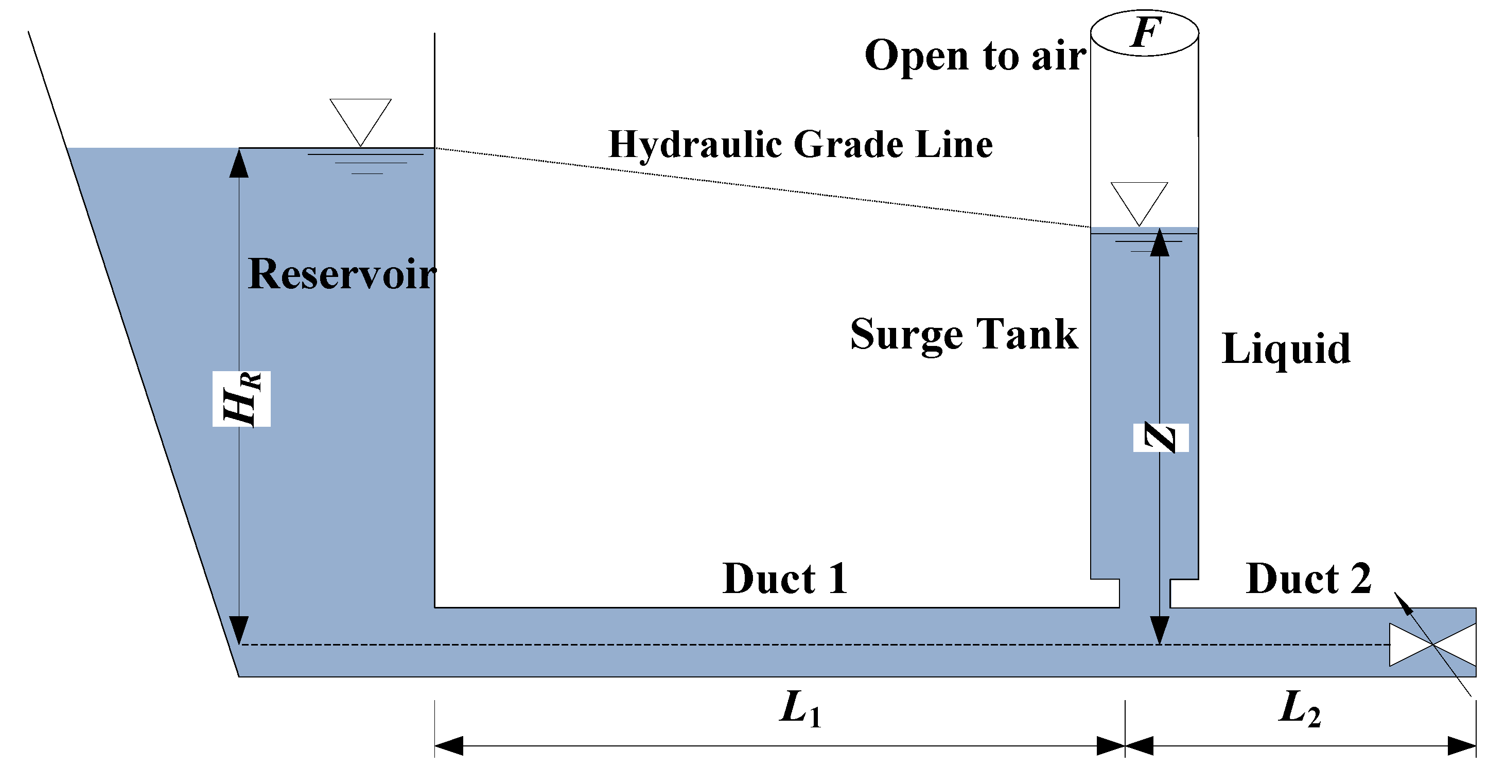
• Case 1: The water level of the reservoir is 10 m, and the valve discharge reduces to zero linearly;
• Case 2: The water level of the reservoir is 80 m, and the valve discharge reduces to zero linearly.

The water surface fluctuations are shown in Figure 14 and Figure 15 for Case 1 and Case 2, respectively. The behavior of the surface fluctuation agree well for the MOI and CFD methods, with a relative error less than 5%, which illustrates that the implicit scheme with dynamic meshes has a similar accuracy as the CFD method when simulating water level fluctuations in an open surge tank. Given that the CFD VOF method includes the gas flow, while the MOI does not include the gas flow, the effect of gas flow can be ignored in such cases. The MOC results differ significantly from the CFD and MOI results. The difference increases as the water level rises from 20 to 80 m, which can be explained by the fact that the CFD and MOI take into account the inertial forces in the tank while MOC does not. The inertial forces increase with the water level in the surge tank. The MOC curve shape is thus preserved, and only shows an offset as the water level increases.

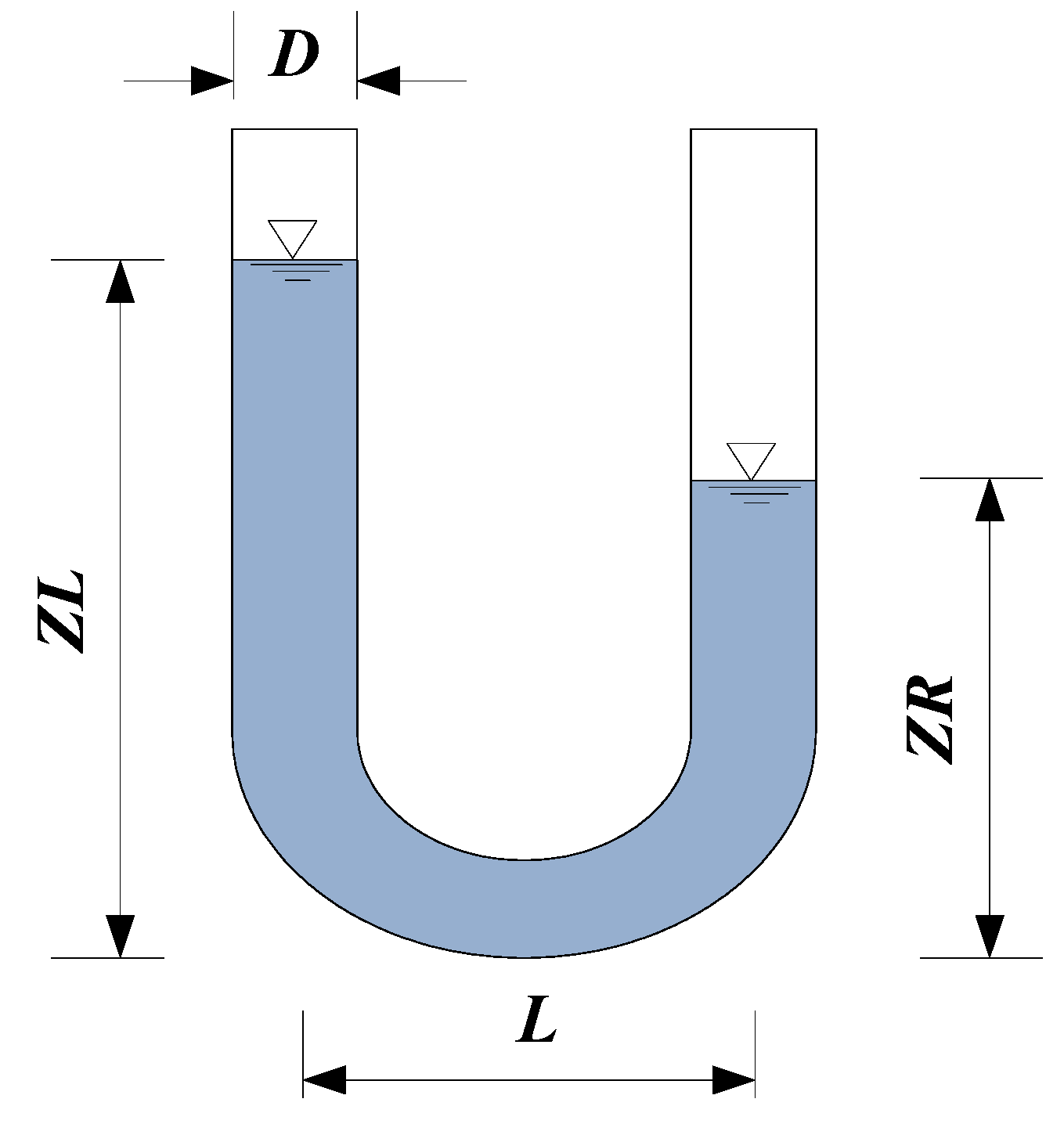
4.1.2. Water Level Fluctuations in a U-tube

Figure 16 shows a U-tube, partly filled with water. The U-tube has an inner diameter D of 2.0 m, a length L between the two vertical sections of 28 m, and a flexion with a semicircular shape. The flow is stationary in the initial state and the water levels ZL and ZR are 40 m and 30 m, respectively. The minor loss due to the bend is not taken into consideration. The liquid flows under gravitational forces, analogous to an open surge tank but with two interfaces. Figure 17 shows the surface elevations when the friction factor f is zero, as in the case of a frictionless wall. The fluctuations never attenuate if the wall is frictionless, showing that there is no significant numerical dissipation. Figure 18 illustrates that the fluctuations decay quickly with increasing friction factor, f.

Figure 14. Oscillation of water level for Case 1.

Figure 14. Oscillation of water level for Case 1.

Figure 15. Oscillation of water level for Case 2.

Figure 15. Oscillation of water level for Case 2.

Figure 16. Schematic diagram of a U-tube.

Figure 16. Schematic diagram of a U-tube.

Figure 17. Water level traces when neglecting friction.

Figure 17. Water level traces when neglecting friction.

Figure 18. Water level traces when considering friction.

Figure 18. Water level traces when considering friction.

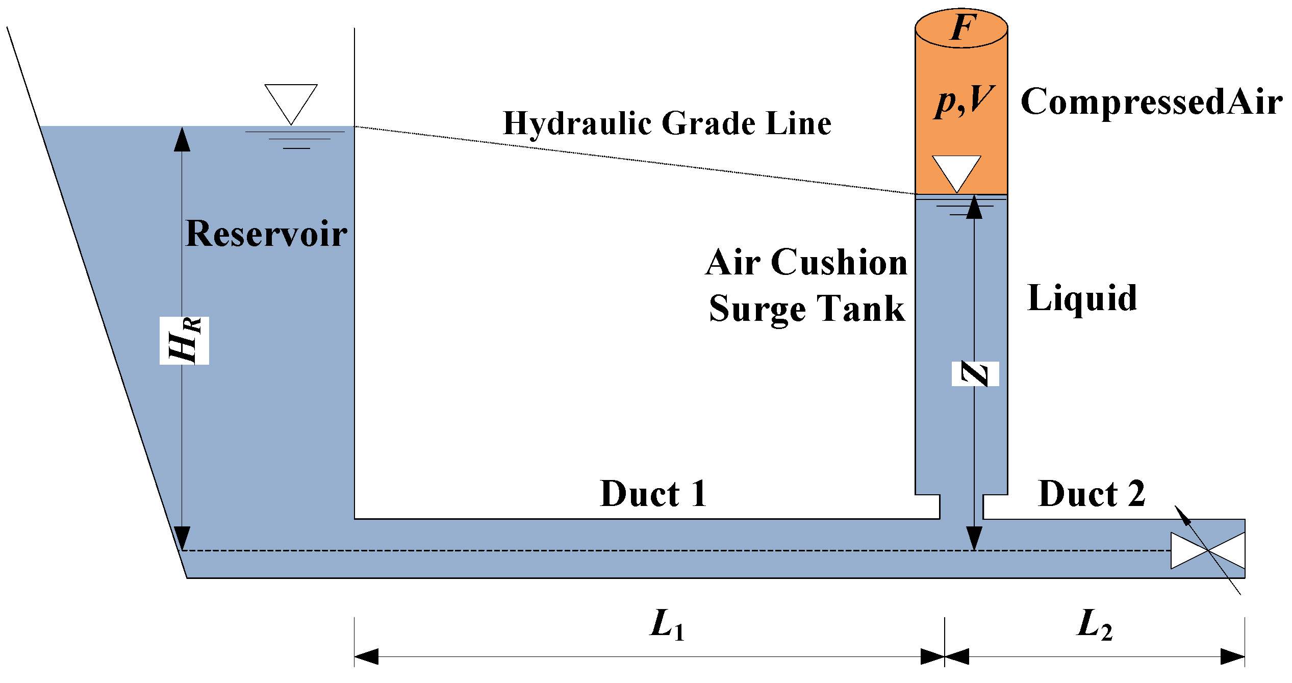
4.2. Gas Phase Limited in a Chamber

In hydropower application, the inner rock wall and the water surface may constitute a closed chamber that stops the gas from escaping, as shown schematically in Figure 19. The water hammer wave is reflected and the water level fluctuations are restrained by the gas compression and expansion due to the change in pressure. In a hydropower station, the length of the diversion tunnel can be shortened and the height of the surge tank can be reduced using an air cushion surge chamber because it is a closed underground structure.

Figure 19. Reservoir-air cushion surge tank-valve system.

Figure 19. Reservoir-air cushion surge tank-valve system.

For water level fluctuations in an air cushion surge tank, as shown in Figure 19, the pressure at the interface is influenced by the gas phase while the water level (yielding the gas volume) determines the gas pressure. The ideal gas state equation is often used to describe the behavior of the gas phase in such a chamber.

A method is here used to model the water level fluctuation in an air cushion surge tank, coupling the implicit scheme using dynamic meshes and the gas state equation. The solution method is similar to that for an open surge tank. However, Step 3 in the algorithm should be replaced by:

$$Z\text{=}{Z}^0\text{+(}{Q}_N\text{+}{Q}_N^0)\text{Δ}t\text{/2}F$$

(34)

$$\text{Δ}{Q}_N=E{E}_N\times \text{Δ}{H}_N+F{F}_N$$

(35)

$$H_N=Z\text{+}\frac{p}{{\text{ρ}}_{W}g}$$

(36)

$$p{V}^n=const$$

(37)

$$V=f(Z)$$

(38)

here, Equation (34) relates the discharge and water level at mesh line N; Equation (35) is the forward scan equation at mesh line N; Equation (36) relates the pressure of the liquid phase head and the pressure of the gas phase at the interface; Equation (37) is the ideal gas state equation; and Equation (38) relates the gas volume and the water level; ρ_w is the water density; V is the gas volume; and n is the polytropic exponent.

For the reservoir-air cushion surge tank-valve system shown in Figure 19, the lengths of Duct 1 and Duct 2 are 100 m and 50 m, respectively, the cross sectional areas for the two ducts and the surge tank are both 1 m². The friction factor is 0.014. The initial steady discharge of the valve is 1 m³/s and the initial gas volume is 20 m³ with a gas pressure of 3.04 bar (3 atm). The valve discharge reduces to zero linearly in 2 s and the transient flow is simulated by the proposed approach with different polytropic exponents n.

Figure 20 and Figure 21 show the oscillations in water level and gas pressure, respectively, with different polytropic exponents in the ideal gas state equation. The wave period and the water level amplitude decrease with increasing coefficient n, while the amplitude of the pressure oscillations in the gas phase increases. If the initial pressure of the gas is 1 atm and the polytropic exponent n is set to 0, the calculation model will neglect the effect of the gas phase and become equivalent to the model shown in Section 4.1.

Figure 20. Oscillation of water level.

Figure 20. Oscillation of water level.

Figure 21. Oscillation of pressure.

Figure 21. Oscillation of pressure.

4.3. Gas Phase Flow in Ducts

In order to reduce the excavated volume in underground hydropower stations, air tunnels are set to extend the underground surge tank to the atmosphere outside the mountain, rather than to heighten the tank vertically to the mountain surface directly, as shown in Figure 22. A surge tank is thus linked to the outside atmosphere by a gas duct with an area far less than that of the surge tank. This may yield a high velocity gas flow during the water surface wave processes. The transient processes in the liquid and gas phases are here simulated by coupling the water hammer equations and gas flow governing equations. Three methods are presented in this section. Method A completely couples the liquid and gas phases, while Methods B and C introduce a simplifying assumption for large gas ducts, where Method A shows that gas phase only slightly affects the liquid phase.

Figure 22. Surge tank with air tunnel.

Figure 22. Surge tank with air tunnel.

4.3.1. Synchronous Coupling of Liquid and Gas Phases (Model A)

As shown in Figure 22, the forward scan for the liquid phase is from the bottom of the surge tank to the water surface. For the gas phase, the forward scan is from the outlet to the surge tank. N and M are thus the last mesh lines of the liquid and the gas meshes. The coupling at the interface is shown in Figure 23.

Figure 23. Coupling between liquid and gas phases.

Figure 23. Coupling between liquid and gas phases.

It is assumed that during a time step ∆t, the inflow-volume of liquid through mesh line N is equal to the outflow-volume of gas through mesh line M, which is expressed as

$$\frac{M_M}{{\text{ρ}}_G}\text{\hspace{0.05em}\hspace{0.05em}\hspace{0.05em}=}{Q}_N$$

(39)

The pressure head of the liquid phase and the pressure of the gas phase can be related as

$$H_N\text{\hspace{0.05em}\hspace{0.05em}\hspace{0.05em}=}Z\text{+}\frac{p_M}{{\text{ρ}}_{\text{G}}g}$$

(40)

The equation relating the water level and the discharge for mesh N can be written as

$$Z={\text{Z}}^{\text{0}}\text{+}\frac{\text{(}{Q}_N^{\text{0}}+Q_N\text{)Δ}t}{2F}$$

(41)

here, M_M and p_M are the mass flow rate and pressure, respectively, at mesh line M for the gas phase; Q_N and H_N are the volume flow rate and pressure head, respectively, at mesh N for the liquid phase; Z is the water-gas surface; ρ_G is the air density; and the superscript 0 indicates a known parameter from the last time step.

There are five unknown parameters in the three Equations (39)–(41), which require two additional closure equations to ascertain the pressure and discharge at a particular mesh lines. The following two equations for the forward scan process can be used for this purpose:

$$\text{Δ}{Q}_N=E{E}_N\times \text{Δ}{H}_N+F{F}_N$$

(42)

$$\text{Δ}{M}_M=E{E}_M\times \text{Δ}{p}_M+F{F}_M$$

(43)

This approach for tracking the water-gas surface fluctuations is similar to that described in Section 4, but different in that a dynamic mesh for the gas phase is considered at the same time.

Consider a reservoir-surge tank-valve system with a gas duct. The lengths of the diversion tunnel and penstock are 500 m and 100 m, respectively, both with a diameter of 10 m. The water level of the reservoir is 80 m and the initial discharge of the valve is 250 m³/s. The area of the surge tank is 200 m² with a resistance coefficient of 0. The air density is assumed to be 1.226 kg/m³ with an operation temperature of 288.15 K. The sound speed in air is 340.4 m/s. The gas flow is stationary initially and the pressure at the outlet is constant at 1.0 bar. The length of the gas duct is L and the diameter is D, which are variable, used to investigate the effect of these two parameter on the results. The transient process is stimulated by closing the valve, which reduces the discharge from 200 m² to 0 over 10 s.

(a) Influence of Duct Diameter

Six gas duct diameters, with a fixed duct length of 1000 m, are here studied using the complete coupling model, and the results are shown in Figure 24, Figure 25 and Figure 26. The maximum and minimum gas pressure in the surge tank are 1.12 bar and 0.92 bar, respectively. This increases and decreases the pressure head by 0.88 m and 0.95 m, respectively, compared with the initial values. As the duct diameter increases, the maximum wind speed at the outlet and the peak pressure in the surge tank of gas phase decreases. The maximum wind speed for a gas duct diameter of 1 m exceeds 30 m/s. Figure 26 shows that the gas phase significantly influences the water level fluctuations. For example, the maximum surge increases while the minimum surge decreases as the gas duct diameter increases.

Figure 24. Effect of duct diameter on gas pressure.

Figure 24. Effect of duct diameter on gas pressure.

Figure 25. Effect of duct diameter on wind speed.

Figure 25. Effect of duct diameter on wind speed.

Figure 26. Effect of diameter on water level fluctuations.

Figure 26. Effect of diameter on water level fluctuations.

(b) Influence of Duct Length

The influence of the gas duct length is here investigated, using the complete coupling model, and the results are shown in Figure 27, Figure 28 and Figure 29. Figure 27 shows that the peak gas pressure in the surge tank increases as the duct length increases. Figure 28 shows that the length of the gas duct has an obvious effect on the maximum wind speed when the duct diameter is small, e.g., when the duct diameter is 1.0 m. The peak value decreases as the duct length increases from 50 to 2000 m. As the duct diameter increases to 3 m or 5 m, the change in peak wind speed is not noticeable when duct length increases. Figure 29 shows that the maximum surge decreases as the duct length increases. However, the trend is not significant when the duct diameter is large, which illustrates that the gas phase has a slight impact on the liquid phase if the gas pressure in the tank changes little in comparison to the initial state because of its large diameter.

Figure 27. Effect of duct lengths and diameters on gas pressure.

Figure 27. Effect of duct lengths and diameters on gas pressure.

Figure 28. Effect of duct lengths and diameters on wind speed.

Figure 28. Effect of duct lengths and diameters on wind speed.

Figure 29. Effect of duct lengths and diameters on water level fluctuations.

Figure 29. Effect of duct lengths and diameters on water level fluctuations.

4.3.2. Neglecting the Effect of the Gas Phase on the Liquid Phase (Model B)

One way to simplify the completely coupled Model A is to neglect the effect of the gas phase on the liquid phase, here referred to as Model B. This makes the numerical simulations of the liquid and gas phases independent. In other words, the wave process of the water level in the surge tank is calculated according to the approach introduced in Section 4.1. Z(t) is then transformed to the time-dependent mass flow rate M(t) of the gas phase by Equation (41), regarded as the inlet boundary condition of the gas duct. The transient flow in the gas duct is then analyzed by the governing equation:

$$M\text{(t)=}F\cdot {\text{ρ}}_G\frac{\partial Z\text{(t)}}{\partial \text{t}}$$

(44)

where F is the area of the surge tank; ρ_G is the density of air; Z(t) is the wave process of the water level in the surge tank; and M(t) is the mass flow rate of the gas duct inlet. The results using Model B are shown and discussed at the same time as those of Model C.

4.3.3. Asynchronous Coupling of Liquid and Gas Phases (Model C)

Another way to simplify the completely coupled Model A is to use a non-deforming mesh for the gas duct, here referred to as Model C. As Equation (35) shows, the pressure at the gas duct inlet acts on the interface, but the gas pressure is replaced by the value of the last time step in this model. The water level fluctuation is then calculated using Z(t), which is converted to the inlet boundary condition of the gas duct by Equation (41). The gas flow is then simulated to obtain the pressure at the gas duct inlet.

The three models, A–C, are all used to calculate the case introduced when analyzing Model A (see Section 4.3.1). Two gas ducts diameters of 1 m and 3 m are here used, respectively, with the same length of 1000 m. The results are shown in Figure 30, Figure 31 and Figure 32, from which three main conclusions can be drawn:

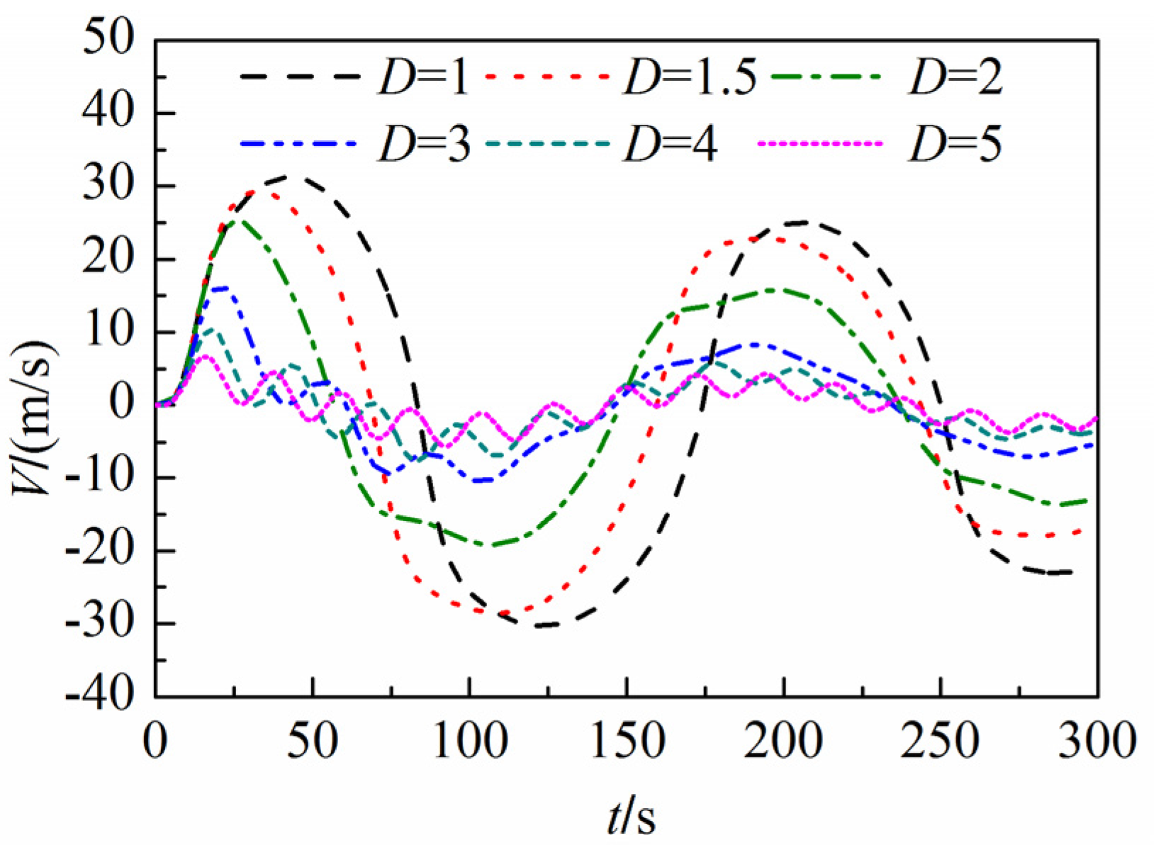
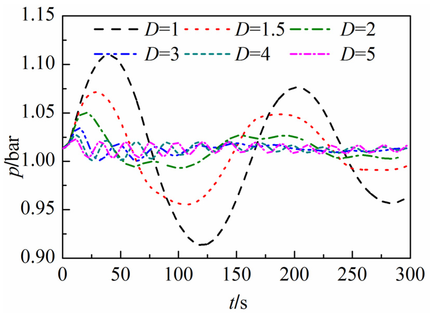
• When the duct diameter is large (e.g., D = 3.0 m), the gas pressure variation in the surge tank is not significant enough to affect the liquid phase. Therefore, traces of gas pressure, water level in the surge, and the gas flow velocity agree for all three models.
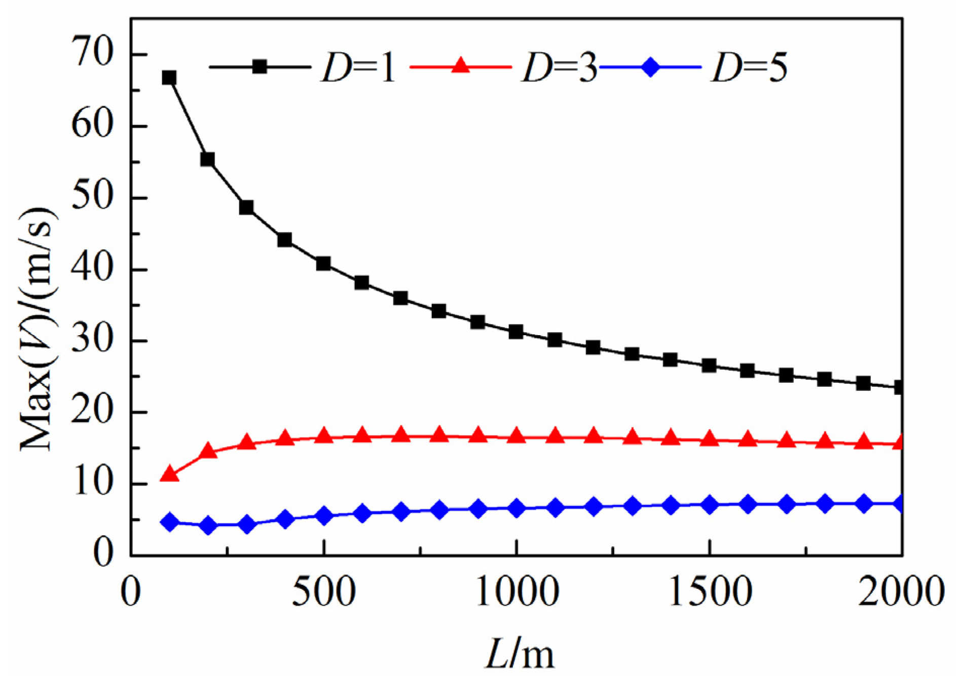
• When the duct diameter is small enough (e.g., D = 1.0 m) such that the gas pressure varies greatly compared to the initial state, the gas behavior during the transient process has a significant influence on the water level fluctuations. However, the water level results calculated by Model B, which neglect the effect of the gas phase on the liquid phase, are unaffected by the variation of the gas duct diameter, so the simulations are not accurate under this circumstance. The peak wind speed at the duct outlet and the maximum gas pressure in the surge obtained by Model B are larger than the results obtained by Models A and C.
• Independent of the change in the gas duct diameter, the water level, the pressure, and the wind speed are very similar for Models A and C. This illustrates that the asynchronous coupling model captures the interaction between the liquid and gas phases as accurate as the synchronous coupling model.

Figure 30. Gas pressure simulated by three models.

Figure 30. Gas pressure simulated by three models.

Figure 31. Wind speed simulated by three models.

Figure 31. Wind speed simulated by three models.

Figure 32. Water level fluctuations simulated by three models.

Figure 32. Water level fluctuations simulated by three models.

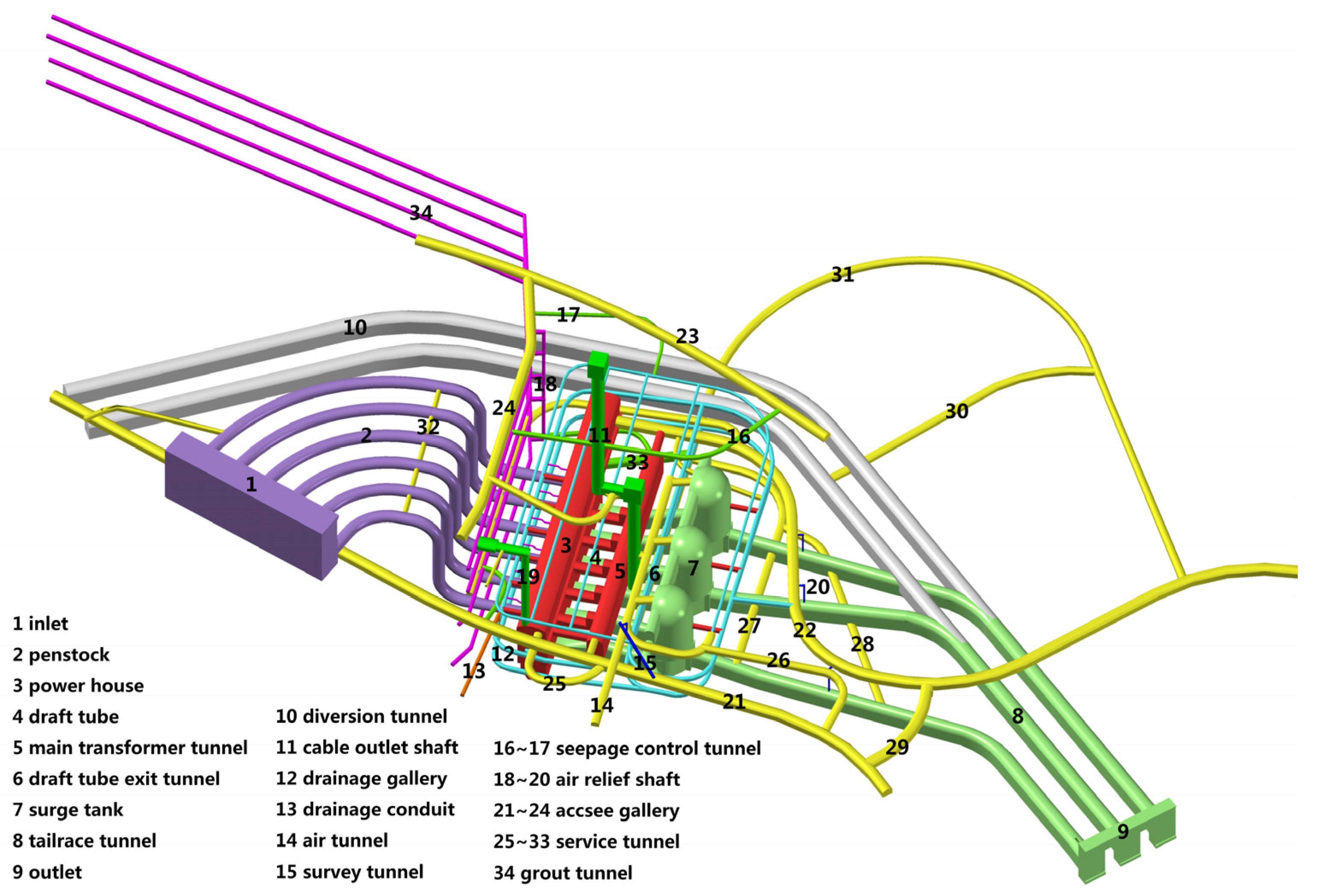
5. An Engineering Application

Figure 33 shows a schematic layout of an underground hydropower station. There are three hydraulic units on the left river bank and each unit includes two Francis turbines. Each turbine has a separate penstock and draft tube, and the two Francis turbines in the same unit share a surge tank and a tailrace tunnel.

Figure 33. Schematic diagram of the piping system of a hydropower station.

Figure 33. Schematic diagram of the piping system of a hydropower station.

Figure 34 shows the presently used computational domain, including reservoirs, intake/outlet, penstock, turbines, surge tanks, tailrace tunnels, and the surge tank air channels. The air channels are used to aerate and provide exhaust as the water level fluctuates in the surge tank, which may be caused by an increase or decrease of the turbine load. Some main parameters of the hydropower station are shown in Appendix B.

Model C is used to simulate the maximum air speed caused by load rejection in the following two cases, and the hydraulic disturbance stimulated by the gas phase flow.

Figure 34. Computational domain.

Figure 34. Computational domain.

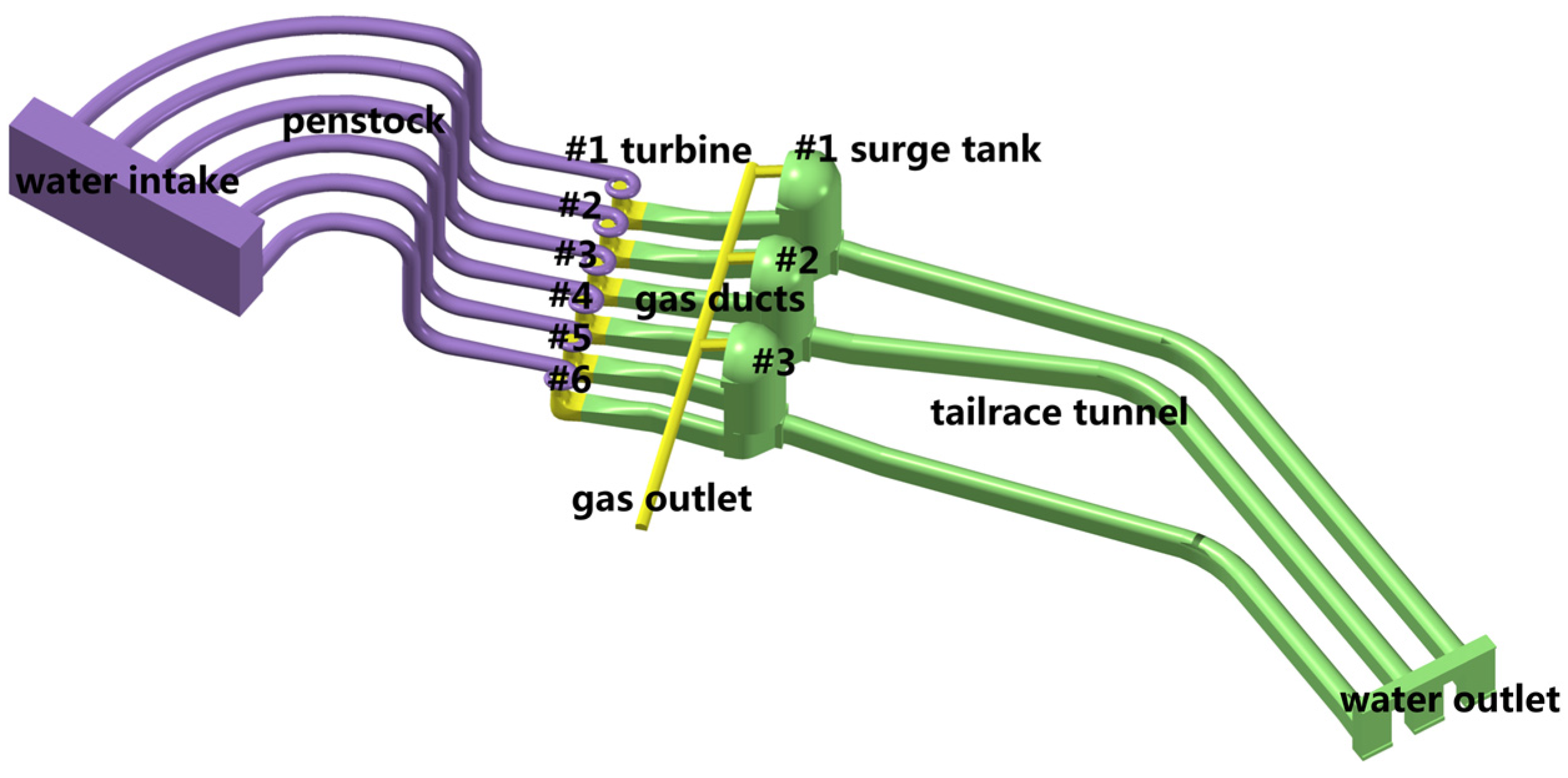
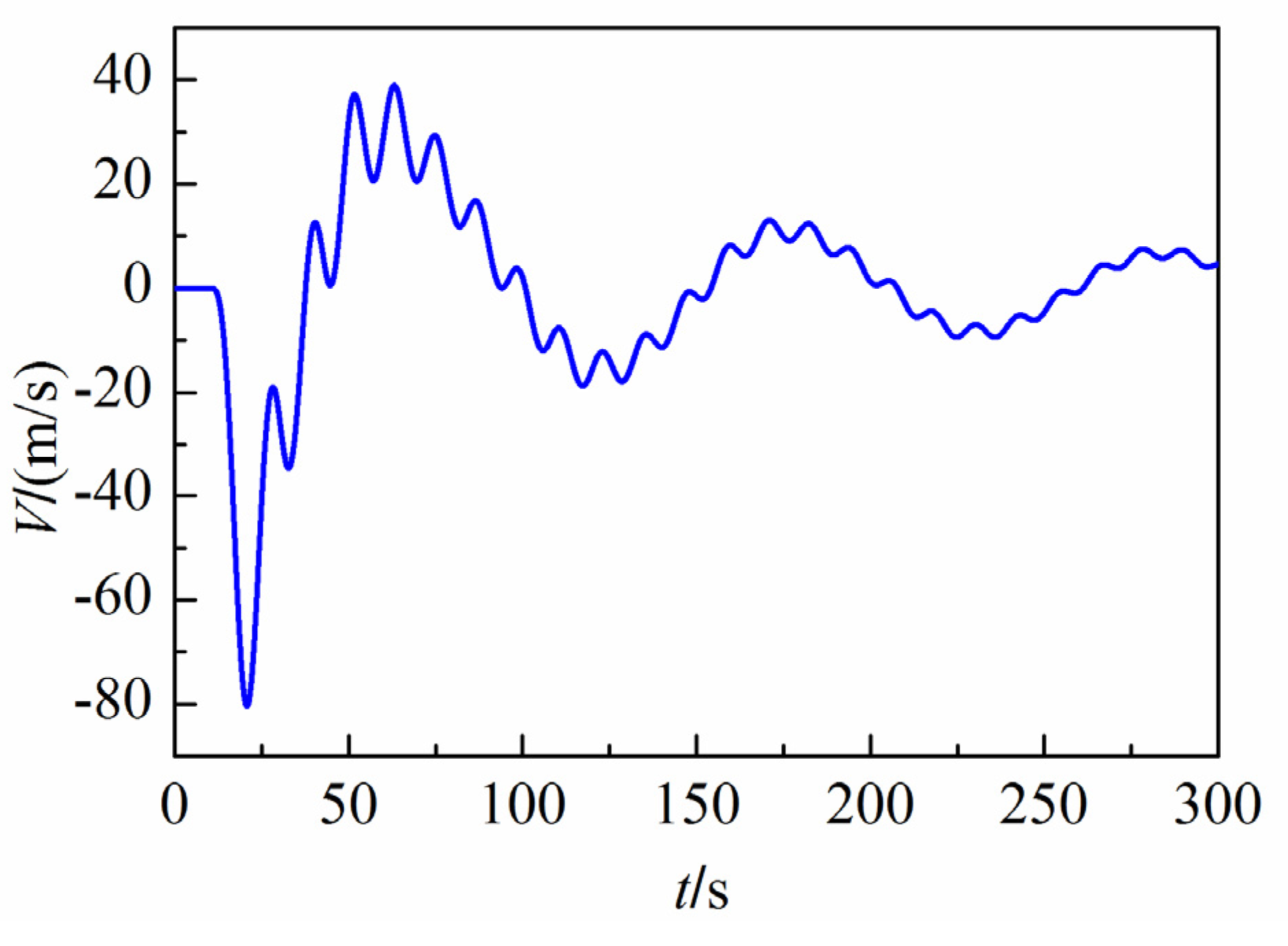
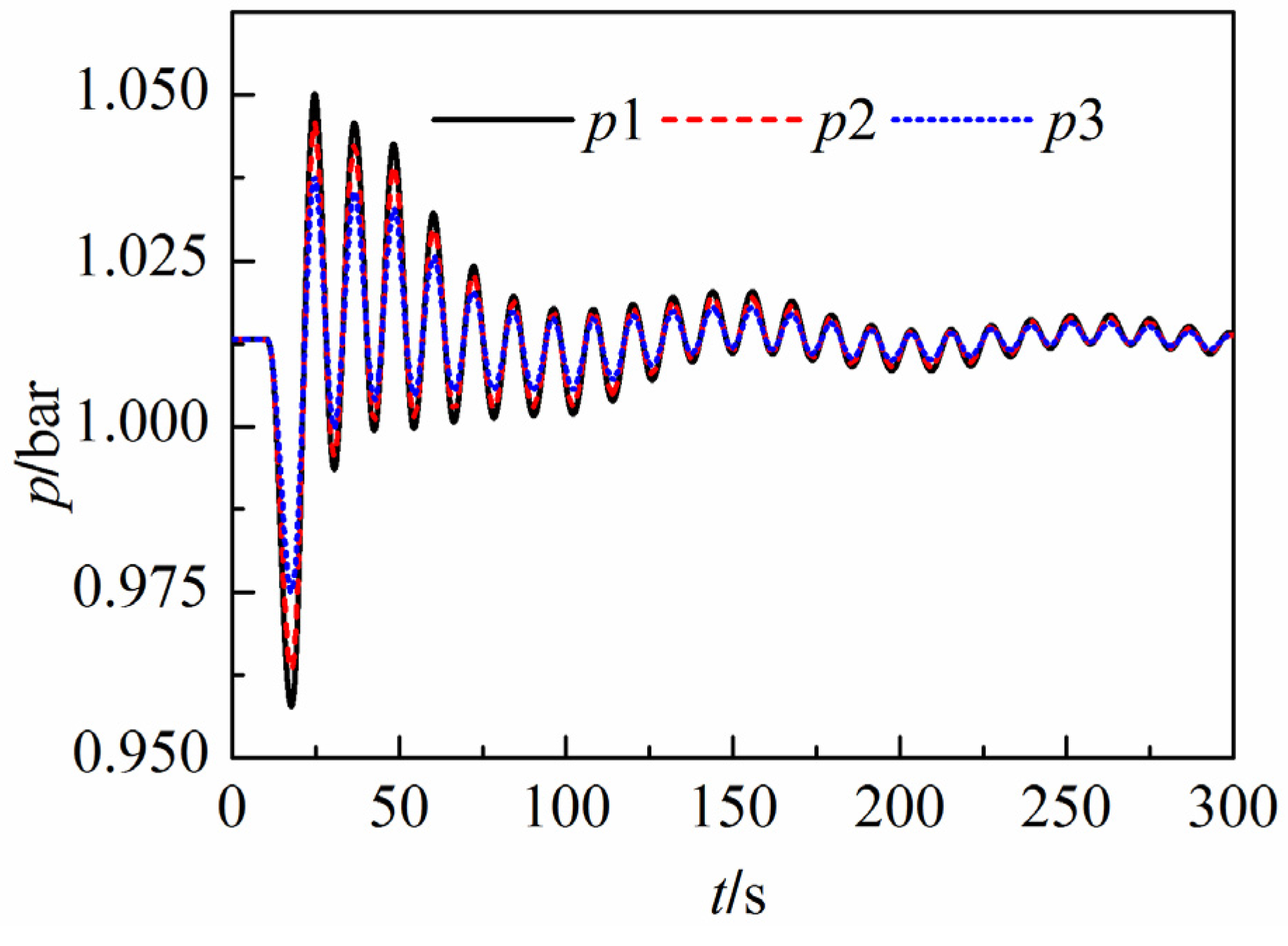
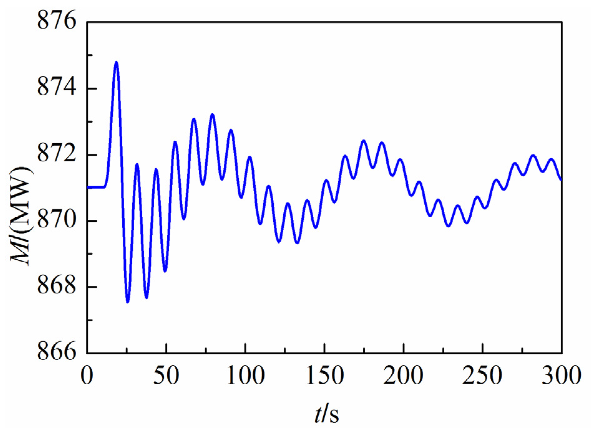
5.1. Case 1: Six Turbines Load Reject Simultaneously

Although it is extremely rare that all turbines reject the load at the same time, a peak mass flow rate would occur in this case because the water level fluctuations in all surge tanks would simultaneously excite the gas flow. The air speed is related to the fluctuation velocity of the water level in the surge tank. A full load rejection is considered here, to predict the extreme values.

Figure 35 shows the gas pressure in the surge tanks during the transient process. The pressure initially decreases because the water level in the tank rapidly drops down due to the load rejection. The air flows into the tank from the outside until the water level reaches the lowest point during this process, and Figure 36 shows that the peak air speed reaches 80 m/s. Emergency load rejection of the turbine is always unpredictable and a large wind speed in the air tunnel poses a great hazard. The air channel should not open to a populated location, to prevent accidents.

Figure 35. Gas pressure in the surge tank for Case 1.

Figure 35. Gas pressure in the surge tank for Case 1.

Figure 36. Wind speed at the outlet for Case 1.

Figure 36. Wind speed at the outlet for Case 1.

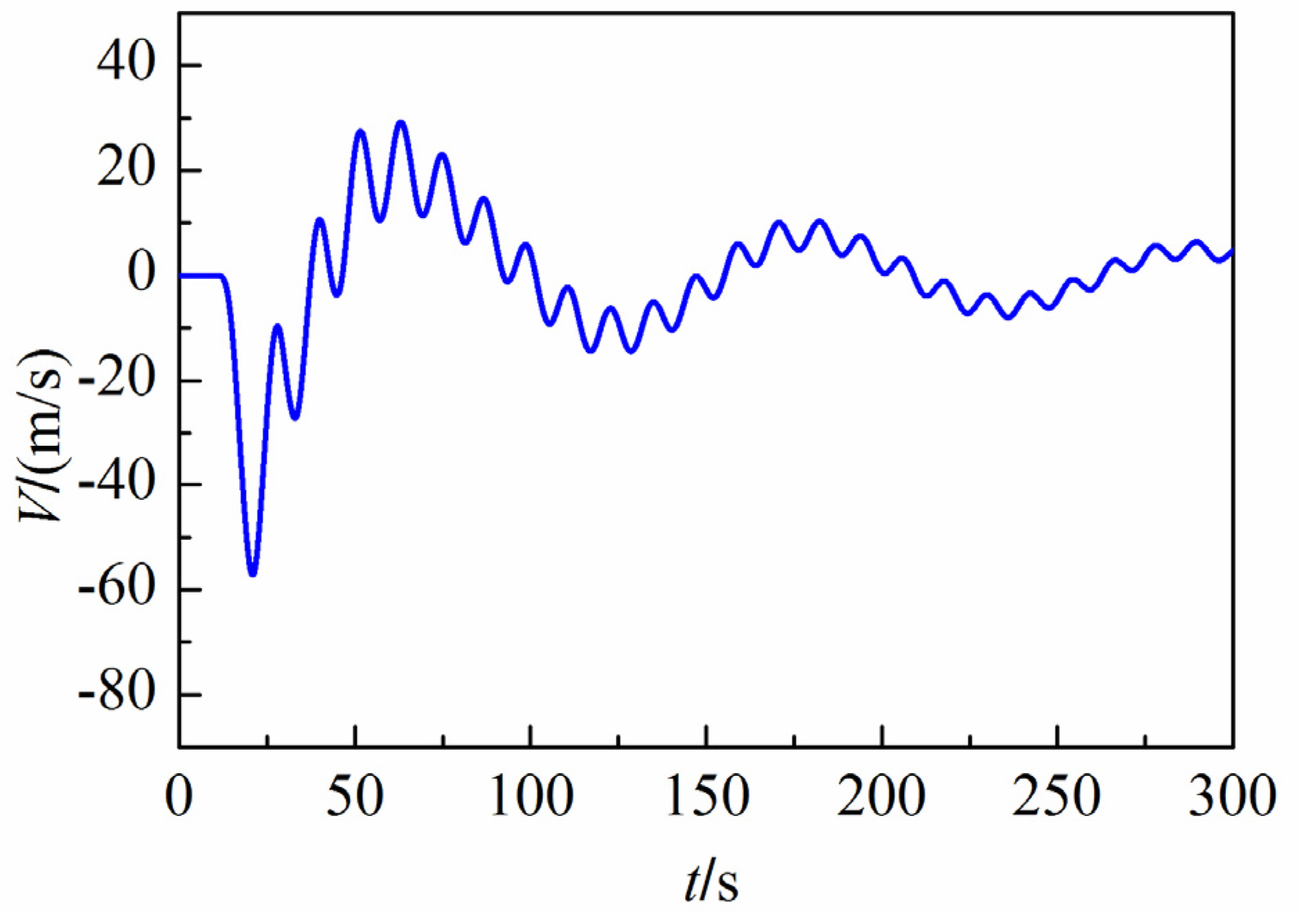
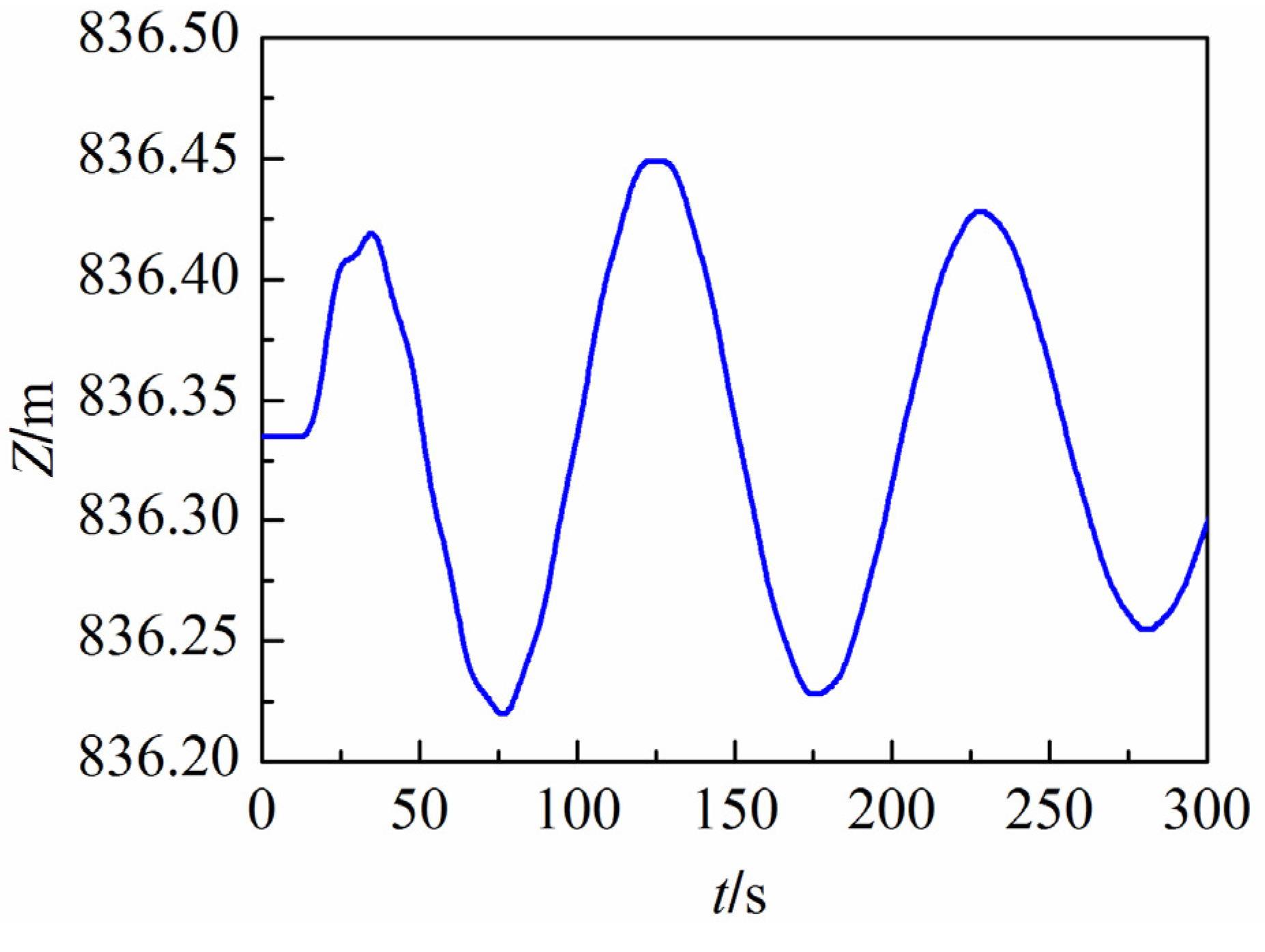
5.2. Case 2: Four Turbines Load Reject and Two Turbines Operate Properly

The three surge tanks are connected by air channels. The transient process caused by increasing and decreasing the load of individual turbines leads to water level fluctuations in the surge tanks, which leads to airflow and pressure changes in the air channels. The air pressure difference acts as an exterior force and affects the water level of the surge tanks. This links back to the turbines that are still running, whose operating heads are changed by the disturbed gas pressure. The power output may subsequently be affected and start to fluctuate during the process. Such a situation is here considered by modeling the effect of load rejection of turbines #1–#4, while continuously running turbines #5 and #6. The guide vanes opening of the two running turbines are assumed to remain constant during the transient process.

Figure 37 shows the gas pressure oscillations in the three surge tanks. The pressure of surge tank #3 yields a dynamic behavior although its turbines are continuously running. Figure 38 presents the wind speed at the outlet. The maximum wind speed is approximately 60 m/s and is far less than the maximum value of 80 m/s in Case 1, where all turbines rejected the load at the same time. Figure 39 shows that there is a slight fluctuation in the water level of surge tank #3. The water level initially increases, since the gas pressure acing on the water surface decreases compared with the initial state. The operating head of the two turbines thus increase initially, which leads to a temporary increase in the output power, as shown in Figure 40. It is obvious that the continuously operating turbines are disturbed by the load rejection of the other turbines, through the air pressure oscillation.

Figure 37. Gas pressure in surge tank #3 for Case 2.

Figure 37. Gas pressure in surge tank #3 for Case 2.

Figure 38. Wind speed at the outlet for Case 2.

Figure 38. Wind speed at the outlet for Case 2.

Figure 39. Water level fluctuation in surge tank #3 for Case 2.

Figure 39. Water level fluctuation in surge tank #3 for Case 2.

Figure 40. Output traces of turbine #5 for Case 2.

Figure 40. Output traces of turbine #5 for Case 2.

6. Discussion

The present work simulates water level fluctuations where the fluid inertia of the liquid and the interaction between the liquid and gas phases are taken into consideration.

The fluid inertia is simulated by the water hammer equations with an implicit difference scheme. Compared with the general approach for water level fluctuation simulations, that treats the tank as a static pressure distribution, the present method can model the dynamic behavior of the water in the tank. This is closer to the real situation but needs more nodes to trace the water level fluctuation. As a result, the fluid inertia of the liquid increases the period while it decreases the amplitude of the fluctuation in the hydropower surge tank system, compared with the method that ignores the fluid inertia. The static pressure distribution method is still useful in some situations, such as in the case of a tank with a large area compared with that of the duct. In such a situation, the fluid inertia in the tank can be neglected because the flow velocity in the tank is small.

The gas phase has a negligible influence on the liquid phase fluctuation if the tank is connected to the atmosphere directly or by short ducts, because the gas pressure cannot increase dramatically at the liquid–gas interface. However, the water level fluctuation may cause huge wind speeds in small-diameter ducts and should be considered for safety reasons if the gas phase wind may come in contact with people.

The mathematical model presented in this work is specified for horizontal water level fluctuations in vertical ducts and tanks, and the applications are mostly focused on hydropower engineering. More complex situations and applications such as slant ducts and free-surface-pressurized flow in horizontal ducts need a more general method.

7. Conclusions

This work numerically studies the water level fluctuations in vertical ducts through a liquid-gas coupling model. An unconditionally stable Preissmann FD scheme, with one weighting parameter, is proposed to calculate the unsteady pipe flow of both the liquid and gas phases. A chasing method is used to solve the implicit linear system. The work comprises the following studies and conclusions.

• Some classic water hammer examples and transient gas flow behavior in pipes and the networks of pipes are solved using the Preissmann method. The reliability and accuracy of the method are verified by comparison with other approaches.
• A dynamic mesh method is applied to the water hammer equations and is used to solve the water level fluctuation in an open surge tank and a U-tube. The model considers the effect of inertial forces and friction in the tank, which is shown to be more precise and physically reasonable compared to other simplified models.
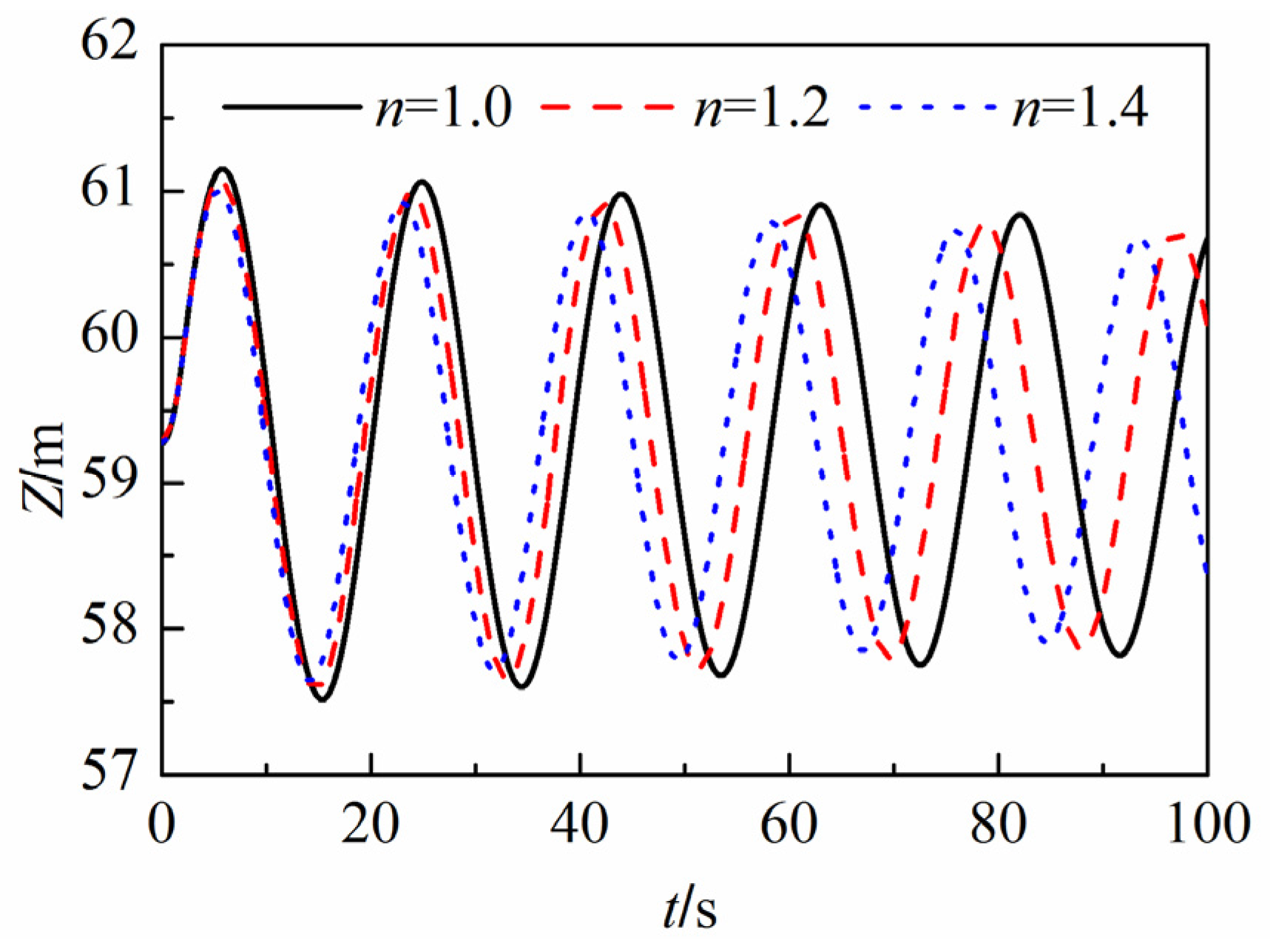
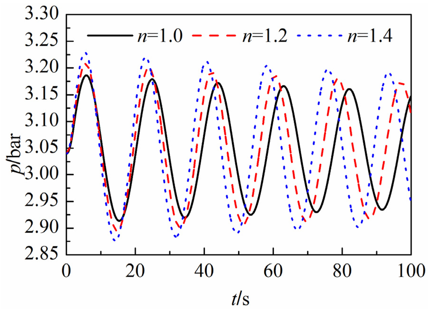
• A model for coupling the water hammer equations and the ideal gas state equations is presented to solve for the water level fluctuation in an air cushion surge tank. The effect of the polytropic exponent for the gas phase is studied.
• Transient flows of liquids and gases in pipelines are solved using the proposed method, and a model for coupling the liquid and gas phases is given to study the interaction between the water level fluctuations and the gas behavior in the duct. Two simplified models are presented and it is shown that an asynchronous coupled model operates as well as the synchronous coupled model.
• The proposed methods are used for the calculation of transient processes in a hydropower station. Peak wind speed in the air channel, and hydraulic disturbances caused by the gas phase, are studied in an engineering project.

References

1. Chaudhry, M.H. Applied Hydraulic Transients; Van Nostrand Reinhold: New York, NY, USA, 1987. [Google Scholar]
2. Wylie, E.B.; Streeter, V.L.; Suo, L. Fluid Transient in Systems; Prentice-Hall: Englewood Cliffs, NJ, USA, 1993. [Google Scholar]
3. Ghidaoui, M.S.; Zhao, M.; McInnis, D.A.; Axworthy, D.H. A review of water hammer theory and practice. Appl. Mech. Rev. 2005, 58, 49–76. [Google Scholar] [CrossRef]
4. Hwang, Y. Development of a characteristic particle method for water hammer simulation. J. Hydraul. Eng. 2013, 139, 1175–1192. [Google Scholar] [CrossRef]
5. Wiggert, D.C.; Sundquist, M.J. Fixed-grid characteristics for pipeline transients. J. Hydraul. Div. 1977, 103, 1403–1415. [Google Scholar]
6. Goldberg, D.E.; Wylie, E.B. Characteristics method using time-line interpolations. J. Hydraul. Eng. 1983, 109, 670–683. [Google Scholar] [CrossRef]
7. Lai, C. Comprehensive method of characteristics models for flow simulation. J. Hydraul. Eng. 1989, 114, 1074–1095. [Google Scholar] [CrossRef]
8. Almeida, A.B.; Koelle, E. Fluid Transients in Pipe Networks; Elsevier: New York, NY, USA, 1992. [Google Scholar]
9. Karney, B.W.; Ghidaoui, M.S. Flexible discretization algorithm for fixed grid MOC in pipeline systems. J. Hydraul. Eng. 1997, 123, 1004–1011. [Google Scholar] [CrossRef]
10. Larock, B.E.; Jeppson, R.W.; Watters, G.Z. Hydraulics of Pipeline Systems; CRC Press: Boca Raton, FL, USA, 2000. [Google Scholar]
11. Holly, F.M.; Preissmann, A. Accurate calculation of transport in two dimensions. J. Hydraul. Div. 1977, 103, 1259–1277. [Google Scholar]
12. Rohani, M.; Afshar, M.H. Simulation of transient flow caused by pump failure: Point-implicit method of characteristics. Ann. Nucl. Energy 2010, 37, 1742–1750. [Google Scholar] [CrossRef]
13. Afshar, M.H.; Rohani, M. Water hammer simulation by implicit method of characteristic. Int. J. Press. Vessels Pip. 2008, 85, 851–859. [Google Scholar] [CrossRef]
14. Chaudhry, M.H.; Hussaini, M.Y. Second-order accurate explicitly finite-difference schemes for water hammer analysis. J. Fluids Eng. 1985, 107, 523–529. [Google Scholar] [CrossRef]
15. Jin, M.; Coran, S.; Cook, J. New one-dimensional implicit numerical dynamic sewer and storm model. Glob. Solut. Urban Drain. 2002. [CrossRef]
16. Pezzinga, G. Quasi-2D model for unsteady flow in pipe networks. J. Hydraul. Eng. 1999, 125, 676–685. [Google Scholar] [CrossRef]
17. Guinot, V. Riemann solvers for water hammer simulations by Godunov method. Int. J. Numer. Methods Eng. 2000, 49, 851–870. [Google Scholar] [CrossRef]
18. Hwang, Y.H.; Chung, N.M. A fast godunov method for the water-hammer problem. Int. J. Numer. Methods Fluids 2002, 40, 799–819. [Google Scholar] [CrossRef]
19. Zhao, M.; Ghidaoui, M.S. Godunov-type solutions for water hammer flows. J. Hydraul. Eng. 2004, 130, 341–348. [Google Scholar] [CrossRef]
20. León, A.; Ghidaoui, M.S.; Schmidt, A.; García, M. Godunov-type solutions for transient flows in sewers. J. Hydraul. Eng. 2006, 132, 800–813. [Google Scholar] [CrossRef]
21. Sabbagh-Yazdi, S.R.; Mastorakis, N.E.; Abbasi, A. Water hammer modeling by Godunov type finite volume method. Int. J. Math. Comput. Simul. 2007, 4, 350–355. [Google Scholar]
22. Greyvenstein, G.P. An implicit method for the analysis of transient flows in pipe networks. Int. J. Numer. Methods Eng. 2002, 53, 1127–1143. [Google Scholar] [CrossRef]
23. Pretorius, J.J.; Malan, A.G.; Visser, J.A. A flow network formulation for compressible and incompressible flow. Int. J. Numer. Methods Heat Fluid Flow 2008, 18, 185–201. [Google Scholar]
24. Wylie, E.B.; Streeter, V.L. Fluid Transients; McGraw-Hill: New York, NY, USA, 1978. [Google Scholar]
25. Osiadacz, A.J. Simulation and Analysis of Gas Pipeline Networks; E. & F.N. Spon: London, UK, 1987. [Google Scholar]
26. Kessal, M. Simplified numerical simulation of transients in gas networks. Chem. Eng. Res. Des. 2000, 78, 925–931. [Google Scholar] [CrossRef]
27. Thorley, A.R.D.; Tiley, C.H. Unsteady and transient flow of compressible fluids in pipelines—A review of theoretical and some experimental studies. Int. J. Heat Fluid Flow 1987, 8, 3–15. [Google Scholar] [CrossRef]
28. Ibraheem, S.O.; Adewumi, M.A. On total variation diminishing schemes for pressure transients. J. Energy Resour. Technol. 1999, 121, 122–130. [Google Scholar] [CrossRef]
29. Zhou, J.; Adewumi, M.A. Simulation of transients in natural gas pipelines using hybrid TVD schemes. Int. J. Numer Methods Fluid. 2000, 32, 407–437. [Google Scholar] [CrossRef]
30. Einfeldt, B. On godunov-type methods for gas dynamics. SIAM J. Numer. Anal. 1988, 25, 294–318. [Google Scholar] [CrossRef]
31. Herrán-González, A.; de La Cruz, J.M.; de Andrés-Toro, B.; Risco-Martín, J.L. Modeling and simulation of a gas distribution pipeline network. Appl. Math. Model. 2009, 33, 1584–1600. [Google Scholar] [CrossRef]
32. Behbahani-Nejad, M.; Bagheri, A. The accuracy and efficiency of a MATLAB-Simulink library for transient flow simulation of gas pipelines and networks. J. Pet. Sci. Eng. 2010, 70, 256–265. [Google Scholar] [CrossRef]
33. Alamian, R.; Behbahani-Nejad, M.; Ghanbarzadeh, A. A state space model for transient flow simulation in natural gas pipelines. J. Nat. Gas Sci. Eng. 2012, 9, 51–59. [Google Scholar] [CrossRef]
34. Ke, S.L.; Ti, H.C. Transient analysis of isothermal gas flow in pipeline network. Chem. Eng. J. 2000, 76, 169–177. [Google Scholar] [CrossRef]
35. Geem, Z.W. Multiobjective optimization of water distribution networks using fuzzy theory and harmony search. Water 2015, 7, 3613–3625. [Google Scholar] [CrossRef]
36. Padulano, R.; del Giudice, G.; Carravetta, A. Experimental analysis of a vertical drop shaft. Water 2013, 5, 1380–1392. [Google Scholar] [CrossRef]
37. Wang, C.; Yang, J.D. Water hammer simulation using explicit-implicit coupling methods. J. Hydraul. Eng. 2014, 141. [Google Scholar] [CrossRef]