Article

Uncertainty in Various Habitat Suitability Models and Its Impact on Habitat Suitability Estimates for Fish

1
Department of Bioenvironmental Systems Engineering, National Taiwan University, Taipei 10617, Taiwan
2
Hydraulic Engineering Office, Public Water Department, Taipei City Government, Taipei City 11008, Taiwan
*
Author to whom correspondence should be addressed.
Water 2015, 7(8), 4088-4107; https://doi.org/10.3390/w7084088
Submission received: 6 May 2015 / Revised: 13 July 2015 / Accepted: 17 July 2015 / Published: 27 July 2015

Abstract

:
Species distribution models (SDMs) are extensively used to project habitat suitability of species in stream ecological studies. Owing to complex sources of uncertainty, such models may yield projections with varying degrees of uncertainty. To better understand projected spatial distributions and the variability between habitat suitability projections, this study uses five SDMs that are based on the outputs of a two-dimensional hydraulic model to project the suitability of habitats and to evaluate the degree of variability originating from both differing model types and the split-sample procedure. The habitat suitability index (HSI) of each species is based on two stream flow variables, including current velocity (V), water depth (D), as well as the heterogeneity of these flow conditions as quantified by the information entropy of V and D. The six SDM approaches used to project fish abundance, as represented by HSI, included two stochastic models: the generalized linear model (GLM) and the generalized additive model (GAM); as well as three machine learning models: the support vector machine (SVM), random forest (RF) and the artificial neural network (ANN), and an ensemble model (where the latter is the average of the preceding five models). The target species Sicyopterus japonicas was found to prefer habitats with high current velocities. The relationship between mesohabitat diversity and fish abundance was indicated by the trends in information entropy and weighted usable area (WUA) over the study area. This study proposes a method for quantifying habitat suitability, and for assessing the uncertainties in HSI and WUA that are introduced by the various SDMs and samples. This study also demonstrated both the merits of the ensemble modeling approach and the necessity of addressing model uncertainty.

1. Introduction

Recognizing that the structure and functions of a stream ecosystem are significantly influenced by flow conditions, previous studies have provided valuable insights into the ecological modeling and assessment of stream habitats [1]. Physical hydraulic models, such as the Physical Habitat Simulation system (PHABSIM) and the River 2D model [2], are useful tools for simulating changes in water depth and velocity at scales that are relevant to stream habitats [3,4,5]. The proficiency of the River 2D model at simulating water depth, current velocity and other riverbed characteristics, such as substrate and cover, means that it is a particularly powerful tool for projecting fish habitat suitability indices (HSI). In addition, it is important to estimate the corresponding weighted usable area (WUA), and further to project potential distributions of fish species in rivers [3]. HSI has been widely used as an index of habitat suitability for species in stream ecological studies [6]. Mesohabitats and stream biota have been shown to be associated with distinct combinations of current velocity and water depth [7]. Some studies have elucidated the correlation between current velocity and depth [7,8], as well as their combined effects in ecological modeling and assessment [9]. Additionally, these two variables are used in species distribution models (SDMs) to estimate HSI values for fish species.
To better understand the relationship between environmental variables and species occurrence, various SDMs have been developed and used in stream ecology; some notable examples, from previous work, include the generalized linear model (GLM) [10], the generalized additive model (GAM) [10,11], the random forest model (RF) [12,13], the support vector machine (SVM) [12], the Fuzzy model [14,15], the artificial neural network model (ANN) [10,12], and a model based on probabilistic neural networks (PNN) [16]. However, no consensus has been reached on an optimal model that is applicable in all relevant situations and suitable for all species since each SDM has its own unique structure and merit [17]. Therefore, the variations among models must be considered; otherwise, the selection of an inappropriate SDM may result in mistaken projections and increased uncertainty.
Uncertainty analysis is particularly important when making habitat-suitability projections [18,19]. When an optimal SDM has not yet been identified for a given species and or geographic extent and spatial resolution, blindly making decisions based on the result of a single SDM, without considering the uncertainty inherent in alternative models, may result in suboptimal management planning decisions [20]. Uncertainty analysis is important for two main reasons [18]. First, understanding of the degree of variability associated with model types can help engineers and decision-makers know where improvements can be made; second, such an understanding can indicate the level of confidence associated with SDM projections. If simulated results obtained using various models with acceptable performance are significantly different from one other, the overall result can be regarded as having high variability (low confidence). Ensemble modeling, where projections of species distributions are generated using several statistical or machine learning techniques together instead of using any single modeling technique, that is, the integration of multiple SDM outputs, is recognized as an important technique in modeling habitat suitability when truly optimal models have not been identified [19,21,22].
In addition to the two dominant variables that are accounted for by HSI, which are current velocity and water depth, spatial pattern and heterogeneity in physical conditions can also affect biological processes. In stream ecosystems, mesoscale interactions between channel morphology [23,24] and discharge [25] generate a heterogeneous hydraulic environment and spatial pattern that provide various in-stream habitats for freshwater biota [26,27]. Greater stream habitat heterogeneity frequently results in greater diversity of aquatic species [23,28] and the improved success and survival of individual species [24,29]. Habitat heterogeneity in rivers can be characterized by the relative proportion of mesohabitats (composition), as well as their spatial arrangement (configuration) and temporal dynamics (variation with discharge) [27,30]. Although the characterization of hydromorphological conditions at an ecologically relevant scale is made possible by quantifying the hydraulic environment of streams via empirical data and an increasing number of models to choose from [27], the quantification of both uncertainty and stream habitat heterogeneity is not so straight forward [12,24]. Additionally, few methods for quantifying variability in SDM outputs are available, not to mention methods for quantifying habitat heterogeneity and relating it to aquatic species ecology [12,24].
This study quantifies the relationship between fish abundance and spatial patterns of mesohabitats using six SDMs, which are the general linear model (GLM), the general additive model (GAM), the random forest model (RF), the support vector machine model (SVM), the artificial neural network model (ANN), and an ensemble model (which yields the average of the outputs of the preceding five SDMs). The objectives of this study are as follows: (1) quantify the relationship between fish abundance (represented by HSI) and flow conditions using SDMs and calculate the weighted usable area (WUA) for the focal species; (2) quantify in-stream spatial heterogeneity of flow conditions and of HSI using information entropy, and (3) quantify the variability of HSI values, WUA locations and the entropy of HSI originating from discrepancies between outputs of various SDMs and the ensemble model approach.

2. Materials and Methods

This study focuses on the relationship between fish abundance and mesohabitat spatial patterns. Specifically, fish occurrence data and the spatial patterns of mesohabitats (based on current velocity V and water depth D data) in the Datuan Stream in northern Taiwan were used in this study. The area was surveyed in the summer of 2008. There were 63 samples collected using backpack electrofishing. The equipment had an effective radial range of 2 m. Water turbulence meant that this method of sampling was most appropriate, due to the difficult in directly observing Sicyopterus japonicas via snorkeling. Stream bank observation was also difficult to perform due to the lack of suitable observation points (i.e., bridges, and other ecological engineering structures). The study area in Datuan Stream was approximately 300 m2. Consistent with previous studies, Sicyopterus japonicas, an amphidromous gobiid, was the focal species, as it has often been identified as a habitat quality indicator species [5,31,32,33]. Lin et al. (2011) [5,32] have described the study area and the method for collecting data in more detail. Figure 1 presents the study area and sampling locations as well as the number of Sicyopterus japonicas observed.
Figure 1. (a) Study site; (b) sample locations and number of Sicyopterus japonicas observed; and (c) Sicyopterus japonicas observations and corresponding stream velocity and depth.
Water 07 04088 g001

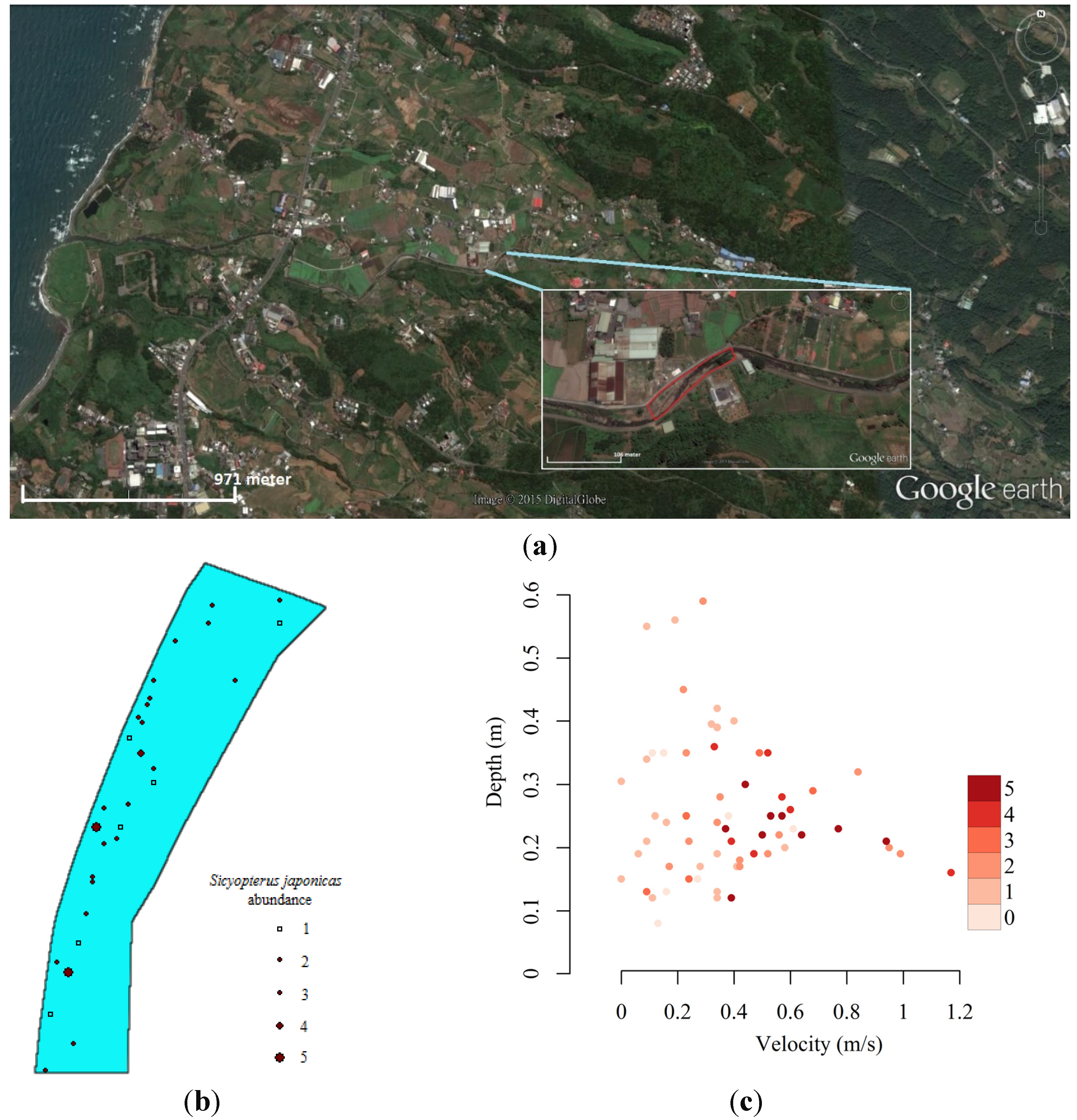
2.1. Hydraulic Model and Model Units

River 2D was used to generate spatial maps of current velocity (V) and water depth (D) across the study area. The spatial resolution of V and D is 4 m2. River 2D is a free-source two-dimensional depth-averaged finite element hydrodynamic model that is used in fish habitat evaluation studies [2]. During the flow condition simulation, geo-referenced topographic measurements and boundary conditions, including flow rate as well as upstream and downstream water levels, were used as input data. The terrain model was based on a triangular network of elements (cells). The sizes of the substrates in the study area were homogeneous and were neglected in estimating HSI.
The model was calibrated by adjusting the bed roughness height to fit the measurements of current velocity (V) and water depth (D) in spring 2008; it was validated using V and D measurements for summer 2008. V and D were classified using the classification criterion that was proposed by Lin et al. (2011) [32]. Both the projected current velocity and water depth across the study area were inputted into the species distribution models.

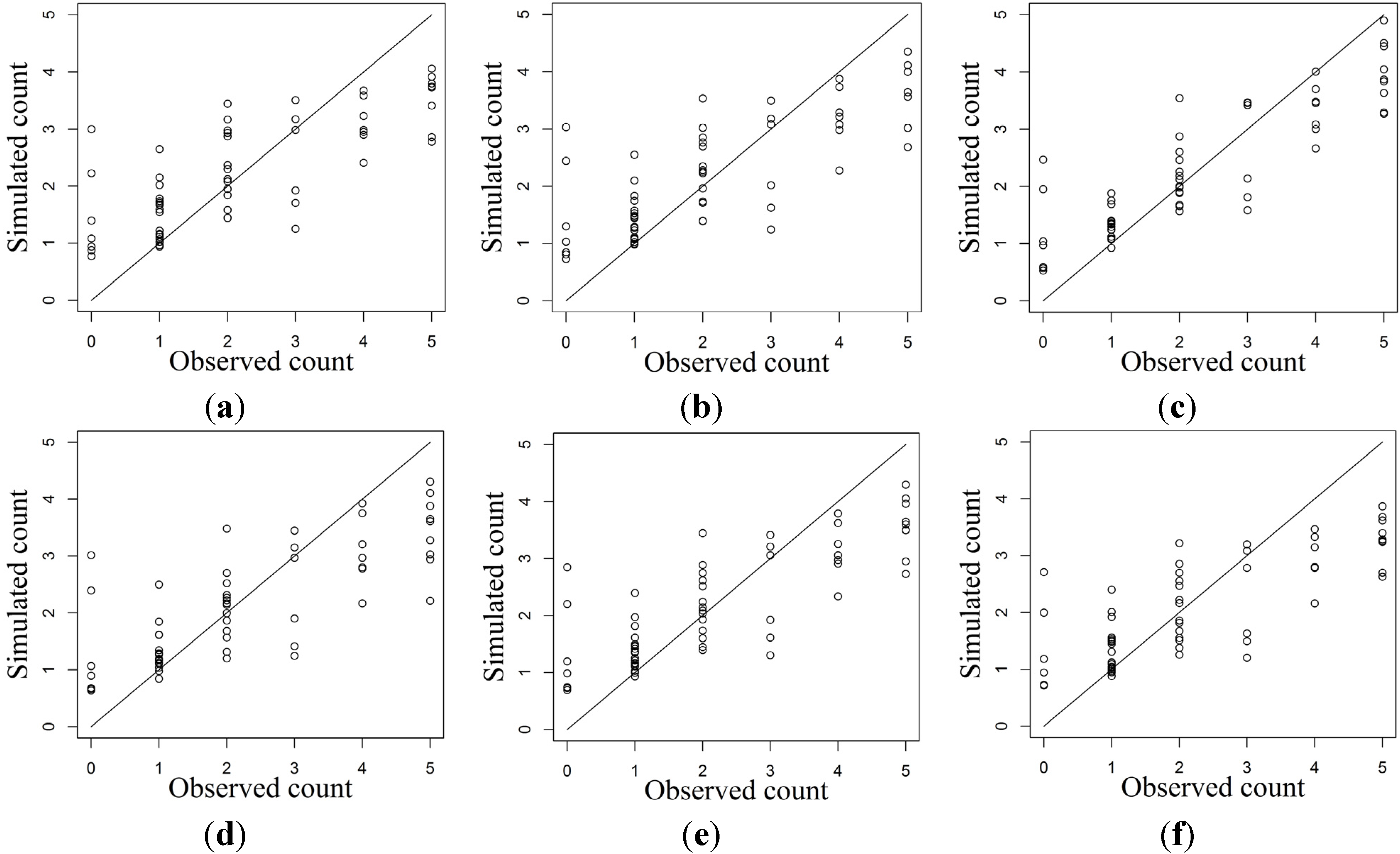
2.2. Ensemble Modeling of Species Distribution and Model Evaluations

The SDMs considered in this study include GLM, GAM, RF, SVM and ANN, which are widely applied to model species distributions [19]. The GLM represents a flexible extension of linear models that connect species abundance to the driving factors of interest using a log link function [34]. Poisson regression is an example of a generalized linear model. The “stat” package of the R software was used to project the abundance of fish at each location using GLM [35]. The GAM is an extension of the general linear models that relate species abundances to the driving factors that are considered to have a polynomial form based on a Poisson distribution with a log link function [36]. The “gam” package of the R software was used to project the fish abundance at each location using GAM [37]. In order to further analyze the species abundance model fit and test the assumptions of the Poisson process, the chi-square test of goodness of fit was applied and the p-value was determined for both GLM and GAM. Random forests (RF) refer to an ensemble machine learning method for classification in which many decision trees are trained using bootstrap replicates of a complete data set [38]. The mean projection of the individual trees is the output. The only assumption of the RF is high representativeness of sampled data. The “random Forest” package of the R software was used to project fish abundance at each location of interest using Random forests [39].
SVM assigns each location to one of the classes y = 0, 1, 2, …, n (where n represents the number of species presences) [8]; the conditions of locations which are more conducive to species are assumed to correlate with a higher number of species presences and vice-versa. A hyperplane which maximizes the margin between the training points associated with the classes, based on the conditions, i.e., driving factors of interest, is obtained via convex quadratic programming [8]. The “e1071” package of the R software was used to project the abundance of fish at each location of interest using SVM [40]. ANNs are non-linear machine learning tools in which a number of neurons are generated to connect species abundance and driving factors, using a back-propagation algorithm [41]. The “nne” package of the R software was used to project the abundance of fish at each location of interest using ANN [42]. There are no assumptions for either machine learning approaches, SVM and ANN. Finally, the results of the ensemble model were defined as the mean of the results of the five SDMs—GLM, GAM, RF, SVM and ANN.
The number of S. japonicas present in each modeling unit was estimated using the five species distribution models (GLM, GAM, RF, SVM and ANN), and the ensemble model (averaging the five SDMs) in terms of two explanatory variables, V and D. V and D generated using River 2D ranged from 0.05 to 1.00 m/s and from 0.05 to 1.25 m, respectively. The measured data were randomly divided into a training set and a validation set, which comprised 70% and 30% of the data, respectively. This split-sample procedure was performed 1000 times per SDM, yielding a total of 6000 outputs. A projection of each species distribution was generated based on the training set. The sampling error was quantified by calculating the sample variance in each training set with a finite population correction factor. Akaike information criterions (AICs) for GLM, GAM, SVM and ANN were calculated, which can be used to deal with the trade-off between the goodness of fit of the model and the complexity of the model [43]. The predictive performance of the models was evaluated in terms of both the root mean square error (RMSE) between the measurements (the 30% validation data) and the projections. Moreover, the standard errors of RMSE were set to the standard deviation of RMSE. Kullback–Leibler divergence (KL) between modeled and observed fish abundance was also derived for each model. This divergence can be used to quantify the information lost by calculating the relative entropy between simulated abundance and observations [43].

2.3. Weighted Usable Area

To obtain the composite habitat suitability for fish, incorporating both V and D, the composite suitability index (HSI, ranging from zero to unity) was calculated for each cell. The V and D values were obtained via River 2D simulations. Specifically, HSI and WUA values were calculated as follows [44]:
H S I i = f ( V i , D i )
W U A = i W U A i = i [ H S I i × A i ]
where f ( V i , D i ) = simulated H S I values as functions of V and D at ith cell; W U A i = weighted useable habitat area in ith cell; and A i = water surface area in ith cell. The WUA values were calculated as a basis of discussing the total potential useable habitat areas and their various discharges. A nonparametric Kruskal–Wallis test and a multiple comparison test were performed to determine whether the median WUA derived from the outputs of the six SDMs differed significantly.

2.4. Spatial Heterogeneity of Flow Conditions and Habitat Suitability

In this study, the spatial heterogeneity of flow conditions and HSI were quantified by calculating the information entropy [12,45]:
Entropy = 1 log 2 ( n c a t ) i = 1 n c a t p i log 2 ( p i )
where ncat is the number of parameter categories considered, and pi is the proportional frequency of the considered parameter in category i. In this case, the entropies of V, D, V + D and HSI were evaluated for each SDM. V ranged from 0.05 to 1.25 m/s and was classed into 12 categories, each with a range of 0.1 m/s. Similarly, D was grouped into ten categories from 0.05 to 1.05 m, defined in 0.1 m increments. HSI was grouped into ten categories from 0 to 1, defined in 0.1 increments. The range of values of information entropy is from zero to one. An entropy value of close to 1 indicates that the considered parameter is distributed uniformly across all categories, indicating high spatial heterogeneity. A value of zero indicates that the considered parameter is concentrated in a single category, indicating a low spatial heterogeneity.
In order to better compare spatial heterogeneity of habitat suitability between models, the mean, standard deviation, median, min, max, range, skewness and kurtosis of information entropy were calculated based on 1000 realizations of each model. Skewness is a measure of the asymmetry of a probability distribution about its mean; in this case, the probability distribution represented information entropy as defined above. To be more specific, if the variables in the distribution are concentrated on the right of the figure, the distribution is said to be left-skewed with a negative value of skewness, indicating that most of the spatial heterogeneity of HSI among 1000 realizations is higher than the mean. Kurtosis is a measure of peakedness of a probability distribution relative to a normal distribution. More specifically, high kurtosis (positive value) represents a sharp peak near the mean of the distribution. In contrast, data sets with low kurtosis (negative value) tend to have a flat top near the mean instead of a distinct peak, indicating the spatial heterogeneity of HSI tends to distribute uniformly.

2.5. Quantifying Variability in Habitat Suitability Index for Each Model

Two sources of uncertainty were considered—that derived from each SDM and that derived from the split-sample procedure with 70% training data and 30% validation data. To elucidate the contributions of these two sources to the variability in HSI, a general linear model is used to quantify their relative contributions by calculating the ratio between the deviation explained by one source and the null deviation [19,46]. Moreover, to evaluate how the degree of similarity between outputs of different models, a principal component analysis (PCA) and Pearson correlation tests were performed on the projections. If the outputs of the models are entirely consistent with each other, then the first principal component (PC1) that is derived from the PCA would explain 100% of the variation. The proportion of the variation that is explained by PC1 can be defined as the degree of variability among model projections. Therefore, PC1 can be regarded as a consensus axis across the projections of species abundance derived from six models [22,47]. So the other extreme example of model consensus would be the situation where the projections show no similarity whatsoever; i.e., they were infinitely inconsistent with each other. In this case, the consensus axis would explain only 16.7% (= 100%/6) of the variance [48]. Accordingly, the variability among projections can be quantified as the inverse of the proportion of variation that is explained by PC1.

3. Results

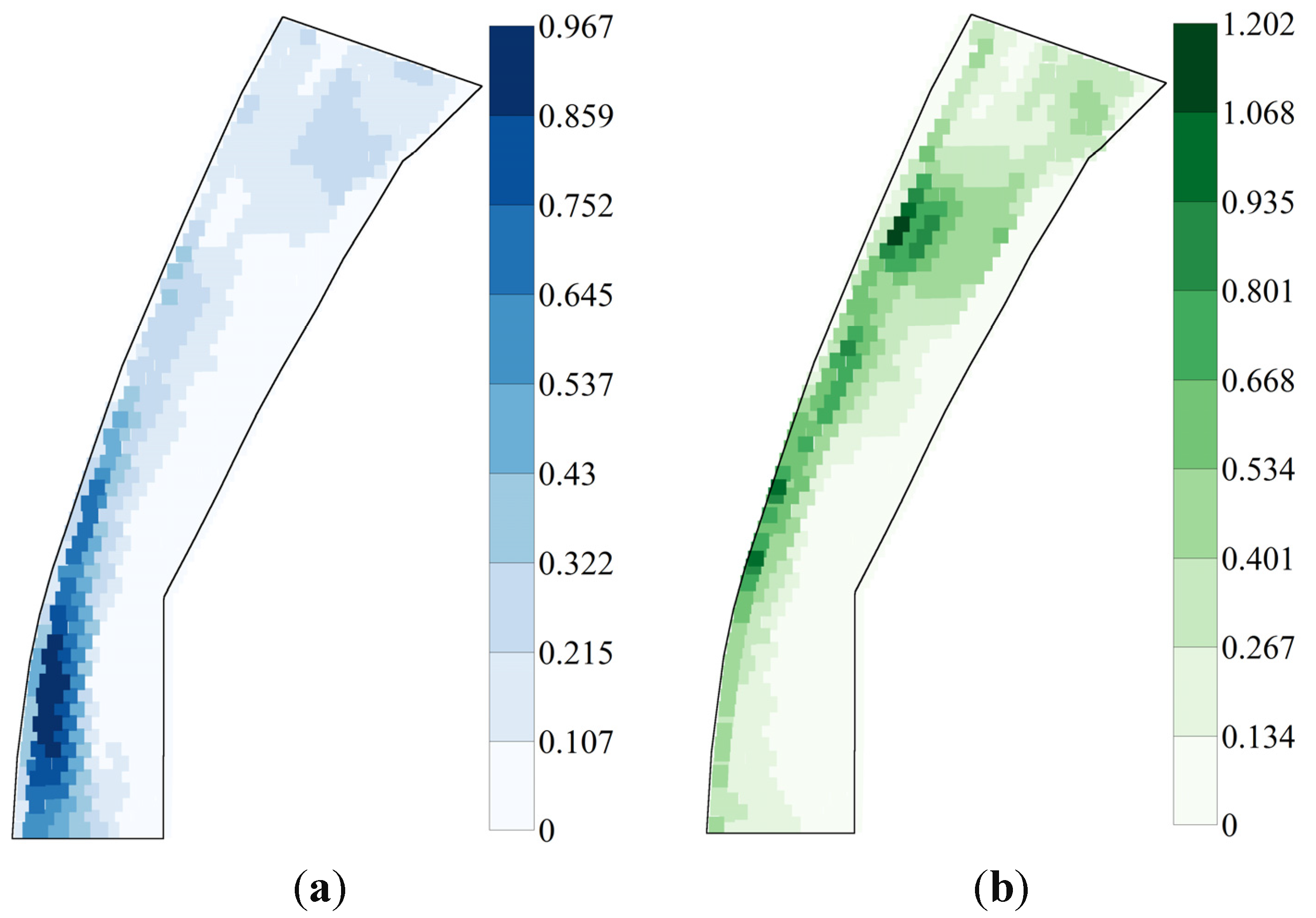
3.1. River 2D Simulations of Flow Conditions

Maps of current velocity and water depth during spring and summer 2008 were simulated by the River 2D model (Figure 2a,b). The flow rate was set to 0.5 m3/s, which was the average of a nearby flow meter. This model was calibrated and validated with the field measurements of flow conditions and its simulation performance are shown in terms of Coefficient of Determination (R2) and Nash–Sutcliffe efficiency coefficient (Eff) [5]. For current velocity, the calibration projection showed an R2 = 0.93 and an Eff = 0.92; the validation dataset showed an R2 = 0.85 and an Eff = 0.84. For water depth, the calibration projection had an R2 = 0.98, and an Eff = 0.98, and the validation projection had an R2 = 0.95, and an Eff = 0.96.
In general, the current velocity decreased and water depth increased from upstream to downstream (Figure 2a,b). The undercut slope of the right bank showed flows with higher velocities (up to 0.97 m/s) and deeper depths (up to 1.2 m), except for the upstream boundary where vegetation grows in gravelly soils. In contrast, the slip-off slope of the left bank resulted in deposition caused by slow, shallow flows. The spatial patterns of V and D were affected directly by the topography of the riverbed. In Figure 2a, the upstream area consisted of areas with high velocity predominantly with few pools in the middle section of the reach close to the right bank where some boulders aggregated. The flows close to gravel-based substrate riverbanks, which were covered with vegetation resulted in low velocity and low depth; other areas in the main channel showed high velocity and low depth. In the downstream section, current velocity was slower and both low and high water depth appeared.
Figure 2. Maps of (a) current velocity (m/s) and (b) depth (m) over the study area. Note: flow direction: South to North.
Water 07 04088 g002

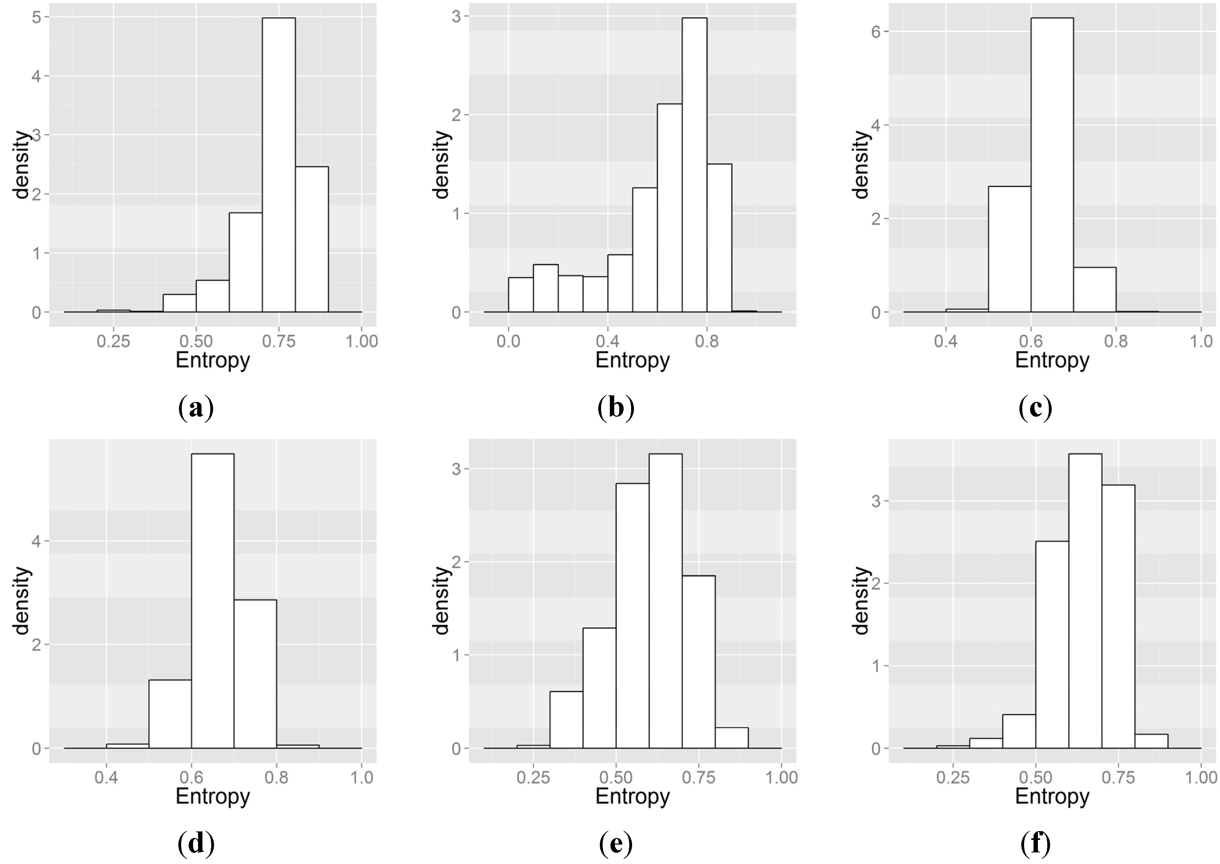
3.2. HSI Obtained from SDMs and Ensemble Models

The p-value of the chi-square goodness of fit test for GLM and GAM were 0.381 and 0.468, respectively. The degree of freedom for GLM and GAM were 57 and 54, respectively. The predictive performance of each SDM in terms of the validation data and the AIC of GLM, GAM, SVM and ANN based on the training data were demonstrated in Table 1. The average RMSEs between the observation and simulation for the six models are 1.505–1.551. The means (standard errors) of AIC for GLM, GAM, SVM and ANN are 72.445 (3.814), 74.313 (3.846), 63.661 (7.407) and 34.805 (5.555), respectively. The average KL between the observed abundance and the simulated results ranged from 0.232 to 0.250. The standard errors of KL for the six models are 0.002–0.003. The model that performed best among the six SDMs, in terms of RMSE and KL, is the ensemble model, which has a RMSE of 1.505 and a KL of 0.232. In contrast, RF underperformed, of which RMSE and KL are 1.562 and 0.247, respectively.
Figure 3 shows the average and standard deviation of HSI projections from 1000 realizations of all six SDM approaches. In this study, the areas with relatively high HSI (more than 0.7) are defined as suitable habitats for S. japonicas. Sites with high average HSI are located in the southwestern part of the study area, regardless of the SDM approach. Similarly, the standard deviation of HSI across all models is concentrated in the southwestern sites except for the SVM outputs in which some of the sites in the north also have high standard deviation of HSI. In terms of driving factor evaluation, current velocity showed a consistent trend (Figure 4). In fact, all model results consistently identified a velocity greater than 0.4 m/s to be highly suitable. The notable differences between SDM algorithms did however become apparent when preferred water depth ranges were taken into account. For instance, while GLM, RF and SVM identified a low water depth (0–0.6 m) as suitable for the focal species, the GAM identified sites with greater water depths (0.8–1.2 m) as high suitability factors. In the case of ANN and ensemble model outputs, there was no clear trend in suitability dependencies on water depth. Therefore, the spatial divergences, which exist between models, are presumably a result of discrepancies between preferred water depths, whereas spatial convergence of model outputs are probably due to similarities in current velocity weighting. By visual inspection of Figure 4, SVM appears to diverge the most; for instance, while GLM, GAM, ANN, and the ensemble model generated smooth general suitability distributions, the SVM model produced outputs, which seem to be far more specific and complicated. This is apparent from the highly nonlinear pattern observed in Figure 4d.
Table 1. Mean ± standard error of validation root mean square error, Akaike information criterion (AIC) and Kullback–Leibler divergence (KL) in 1000 realizations as well as the partial explanations power. * from velocity and depth in the training model.
Model PerformanceGLMGAMRFSVMANNEnsemble
RMSE1.551 ± 0.2121.518 ± 0.2181.562± 0.2211.531 ± 0.2211.517 ± 0.2081.505 ± 0.206
AIC72.445 ± 3.81474.313 ± 3.84663.661 ± 7.40734.805 ± 5.555
KL0.250 ± 0.0880.240 ± 0.0860.247 ± 0.0840.249 ± 0.0930.234 ± 0.0810.232 ± 0.081
V+ D*30.90%39.00%74.10%33.80%32.60%37.20%
V*22.60%23.20%62.90%21.70%19.30%22.50%
D*8.30%15.80%11.60%12.10%13.70%14.60%
To be more specific, GLM evaluated a velocity greater than 0.2 m/s and a depth lower than 0.6 m to be suitable. The GAM-based surface indicated suitable sites with velocity greater than 0.4 m/s and depth larger than 1 m. In RF, a velocity greater than 0.4 m/s and a depth between 0.2 and 0.4 m were evaluated as suitable. SVM-derived HSI distributions showed high habitat suitability in velocities greater than 0.2 m/s and in depths between 0.15 and 0.45 m; this heightened specificity resulted in a far more fragmented projection of suitable habitats, since sites in the immediate vicinity of highly suitable areas tended to have velocities and depths outside of the suitable range. In ANN, the HSI distributions displayed high habitat suitability in velocities greater than 0.3 irrespective of water depths. The distribution from the ensemble model integrated all of the HSI patterns from the five above-mentioned SDMs. It demonstrated two central conditions for high habitat suitability around 0.3 m and 1.1 m in depth, both with a velocity greater than 0.3 m/s. As for the standard deviations of HSI, in GLM, ANN and the ensemble model, the standard deviations follow the trends of average HSI surfaces; that is, in general, the sites with high suitability corresponded to greater standard deviations of HSI. The exception to this was the GAM-based HSI distributions, which indicated high standard deviation in velocities greater than 0.3 m/s and in depths between 0.2 and 0.4 m. Moreover, in RF, the sites with low standard deviations were located in velocity greater 0.3 m/s and in depth between 0.2 and 0.4 m. In SVM, the low standard deviation corresponded to the high HSI values.
Figure 3. Maps of average Habitat suitability index (HSI) derived from (a) GLM; (b) GAM; (c) RF; (d) SVM and (e) ANN; as well as (f) the ensemble model, and maps of standard deviation of HSI derived from (g) GLM; (h) GAM; (i) RF; (j) SVM and (k) ANN; as well as (l) the ensemble model.
Water 07 04088 g003
Figure 4. Habitat suitability surfaces obtained using six species distribution models, (a) GLM; (b) GAM; (c) RF; (d) SVM; (e) ANN; and (f) ensemble model as well as their corresponding standard deviations: (g) GLM; (h) GAM; (i) RF; (j) SVM; (k) ANN; and (l) ensemble model. Note: X-axis represents velocity (m/s), ranging from 0 to 1, and Y-axis represents depth (m) ranging from 0 to 1.2.
Water 07 04088 g004
Figure 5. Scatter plots between observed and simulated fish abundance: (a) GLM; (b) GAM; (c) RF; (d) SVM; (e) ANN and (f) the ensemble model. Note: X-axis represents observed count ranging from 0 to 5, and Y-axis represents simulated count ranging from 0 to 5.
Water 07 04088 g005

3.3. Spatial Heterogeneity of Flow Conditions and of HSI

The information entropies of current velocity and water depth are 0.62 and 0.60, respectively, which indicates moderate spatial heterogeneity. An entropy value of current velocity and depth close to 0.5 represents intermediate spatial heterogeneity of flow conditions over the river. In addition, Figure 6 demonstrates the density distribution of information entropy of HSI in 1000 realizations derived from six different SDMs, including GLM, GAM, RF, SVM, ANN, and the ensemble models. In comparison to the results of the other models, the entropy level of the GAM outputs reveals a far more scattered distribution. In contrast, the distribution of the entropy in RF, SVM and the ensemble models were more consistent. Table 2 shows the entropies of HSI in GLM, GAM, RF, SVM ANN, and the ensemble models ranging from 0.18 to 0.89, 0.03 to 0.89, 0.45 to 0.80, 0.46 to 0.84, 0.29 to 0.85 and 0.04 to 0.83, respectively. The average entropy in GLM was the greatest (0.74) one among all models, while that in ANN was the lowest (0.59). The entropy in GAM and RF had the largest (0.23) and smallest (0.05) standard deviations, respectively. In addition, skewness of the entropy in RF and GLM were greatest (–0.08) and lowest (–1.67), respectively. Furthermore, kurtosis of the entropy in GLM and ANN were the greatest (3.68) and lowest (–0.46), respectively.
Figure 6. Density distribution of information entropy of HSI (1000 runs) obtained using (a) GLM; (b) GAM; (c) RF; (d) SVM; (e) ANN; and (f) the ensemble models. Note: X-axis represents entropy, and Y-axis represents density.
Water 07 04088 g006
Table 2. Descriptive statistics for information entropy of habitat suitability in six models in 1000 realizations.
ModelMeanStandard DeviationMedianMinMaxRangeSkewKurtosis
GLM0.740.090.760.180.890.71–1.673.68
GAM0.600.230.690.030.890.85–1.05–0.06
RF0.630.050.630.450.800.35–0.080.03
SVM0.670.060.670.460.840.38–0.22–0.36
ANN0.590.120.600.290.860.57–0.21–0.46
Ensemble0.640.100.660.040.830.79–1.031.93

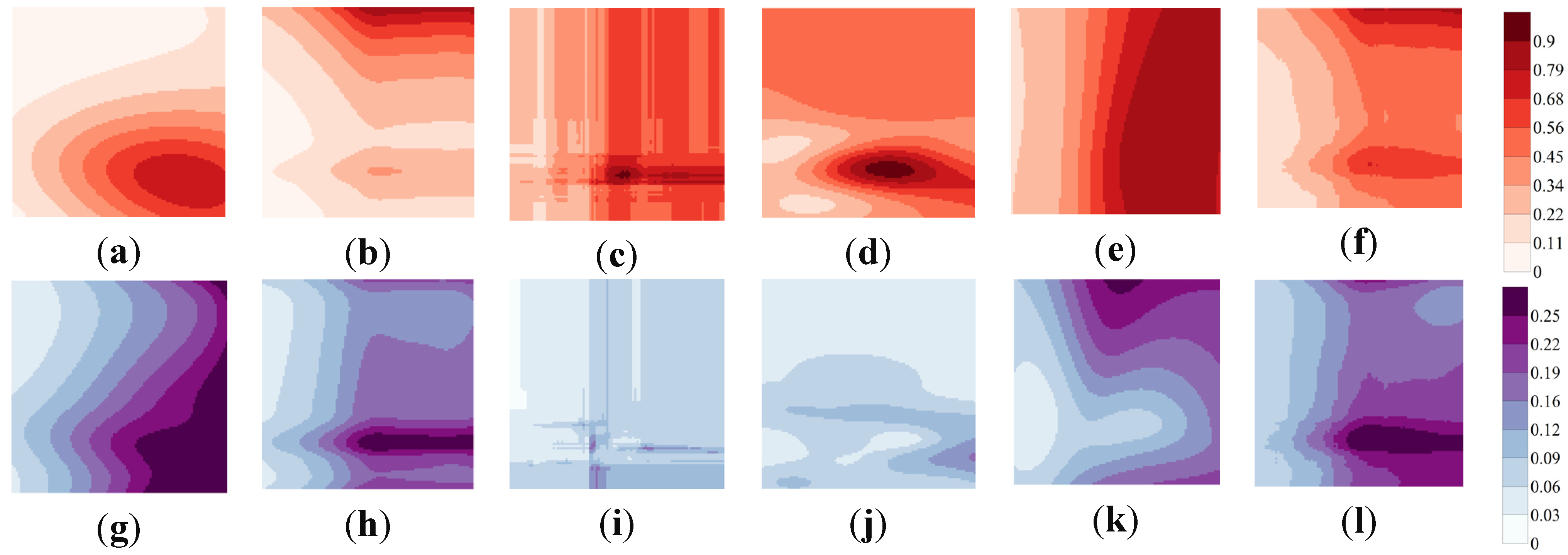
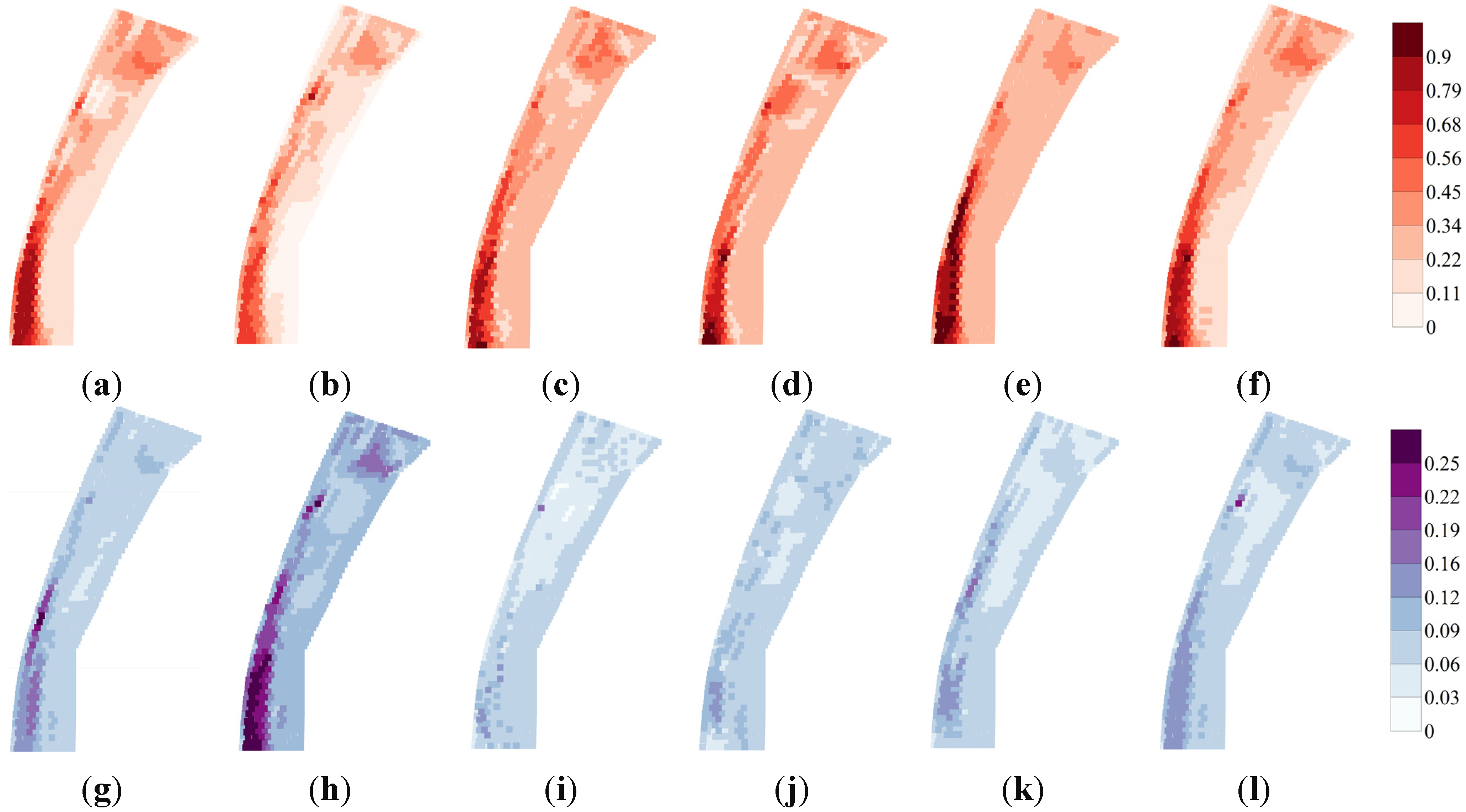
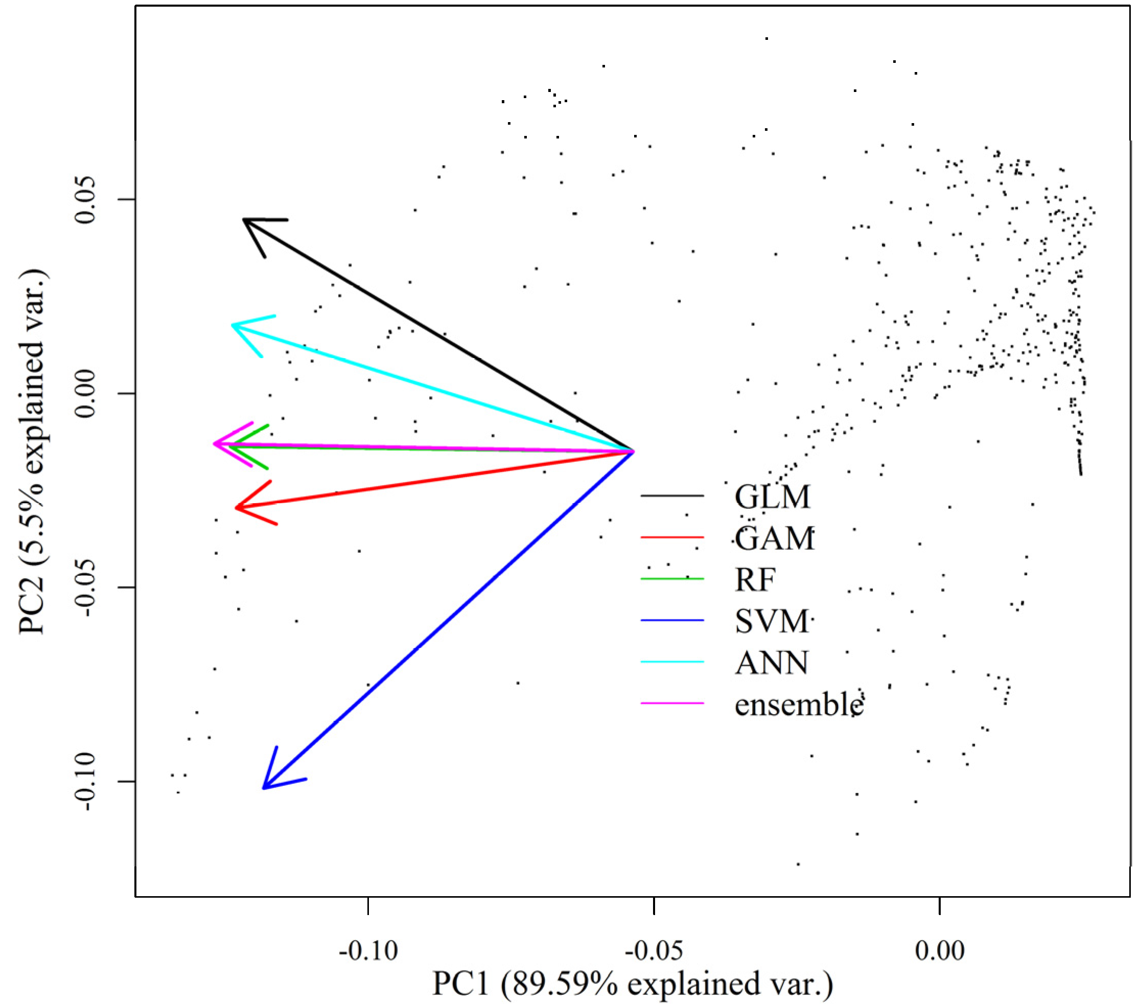
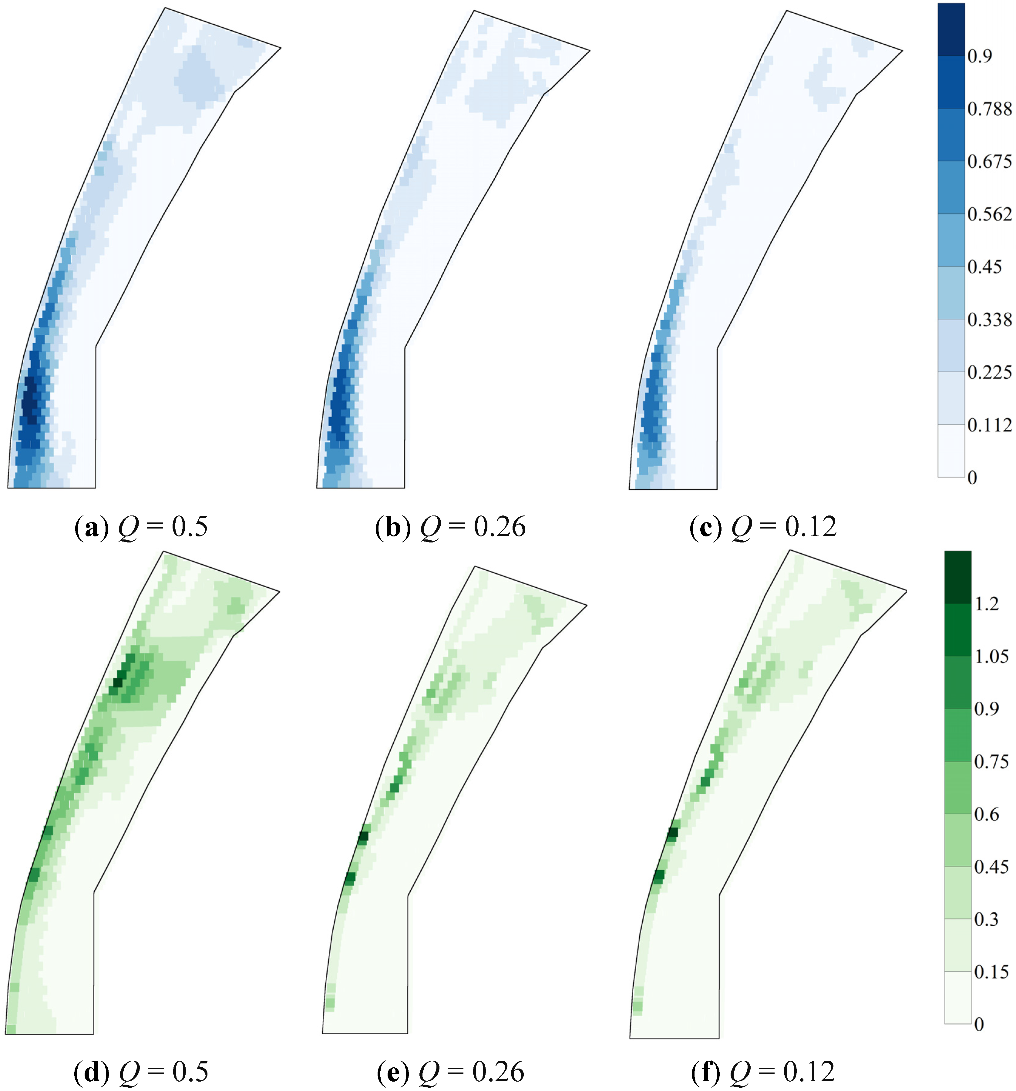
3.4. Variability in Maps of HSI and WUA

The results obtained using the SVM differed the most from the other five models, as quantified by the Spearman correlations, which were 0.70, 0.83, 0.84, 0.77 and 0.87 (Table 3). The remaining five models yielded more mutually consistent results, with mutual correlations of 0.85 to 0.96 (Table 3). In addition to the Spearman correlation, Figure 7 shows the PCA values of HSI that were derived using the six models, which show that the component loadings obtained using SVM, PC1 and PC2, differ distinctly from those obtained using the other models. In contrast, the ensemble model was highly consistent with RF, GAM and ANN in terms of both the Spearman correlation and the component loadings of PC1 and PC2. Since the ensemble models are based on each of the component models, the strong correlation it displays comes as no surprise. Additionally, the model structure and the split-sample procedure explained 63.0% and 37.0% of the variance between 6000 outputs (6 SDMs × 1000 iterations). This was determined by calculating the ratio of the deviation that was explained by any single source and the null deviation that was explained using a general linear model. The sampling error in 1000 subsample iterations ranged from 0.114 to 0.150, of which the mean and standard deviation were 0.133 and 0.006, respectively. The total potential usable areas (represented by WUA) for S. japonicas were calculated for all of the realizations. The means (standard deviations) of WUA obtained using GLM, GAM, RF, SVM and ANN, and the ensemble model were 83.58 m2 (17.28), 68.06 m2 (32.44), 101.05 m2 (13.57), 106.32 m2 (15.70), 106.61 m2 (16.03) and 99.68 m2 (20.40), respectively. The result of Kruskal–Wallis test showed significant differences between WUA obtained using six SDMs (p-value < 0.001). In addition, the multiple comparison test indicated that all of the WUA derived from six models are significantly different from one another, except for those derived from RF and ensemble model, and between SVM and ANN.
Table 3. Correlation of HSI between six models.
ModelGLMGAMRFSVMANNEnsemble
GLM0.850.880.700.910.93
GAM0.870.830.870.96
RF0.840.910.96
SVM0.770.87
ANN0.96
Ensemble
Figure 7. Biplots of HSI and component loadings obtained using six models.
Water 07 04088 g007

4. Discussion

4.1. Usefulness of River 2D in Simulating Flow Conditions

Data on current velocity V and water depth D were collected from fall 2007 to summer 2008 and the spatial patterns of mesohabitats, based on species data collected over a good portion of the study area, were studied further. A 2D numerical hydrodynamic model, River 2D, was used to generate spatial maps of current velocity (V) and water depth (D) over the entire study area. The accuracy of the simulation depended strongly on the quality of bed topography data [49]. In this study, the simulated results showed strong agreement with the empirical data, supporting River 2D’s applicability to small scale analysis [12]. Based on the accuracy of simulated flows, the suitability of the habitat for S. japonicas can be evaluated with confidence over the entire study area.

4.2. SDM-Determined Suitability of Habitat with Respect to Spatial Heterogeneity

A higher AIC represents greater amount of information lost, or the overfitting of a model (too many parameters considered) based on the training dataset. Shearer et al. (2015) found that GAMs based on high-flow rivers overestimated the effects of flow allocation relative to those based on low-flow rivers [11]. In this study, GLM and GAM yielded higher AICs but used fewer parameters, indicating the projections derived from both models lead to greater amounts of information loss in comparison with SVM and ANN. The numbers of parameters for GLM, GAM, ANN and SVM were 5, 8, 9 and 50, respectively. In the case of the two artificial intelligence models, these parameter numbers are dependent on the number of weights in ANN [50] and the number of margin support vectors in SVM [51]. The parameter numbers also suggest that both GLM and GAM suffered from greater information loss than did the other models; while there is a high chance of over fitting in SVM because it included far more parameters than any other model. ANN yielded projections with relatively low RMSE and KL between the predicted and the measured number of species compared to the other models. Considering RMSE simultaneously measures both bias (accuracy) and precision (variation) of the projections; and KL values based on the validation dataset can be used to assess the differences between the distribution of simulated abundance and empirical measurements, this result indicates the merit of the nonlinear transfer function in ANN [52]. Despite this, in terms of the RMSE and KL, the ensemble model outperformed all other single-model approaches considered in this study. Accordingly, the ensemble model has potential to improve upon the predictive performance of all single-model SDMs [22,53].
Schweizer et al. (2007) and Ayllón et al. (2009) emphasized the mutual dependency between flow velocity and depth [7,9]. In this study, HSI was obtained using six species distribution models, which only considered V and D throughout simulations. Based on the criterion of Lin et al. (2011) [5] for classifying mesohabitats, the preferred mesohabitats of S. japonicas, those with high HSI values, were found to be riffles and runs, i.e., those associated with high current velocities [31] presumably due to the fact that mesohabitats with higher current velocities resulted in greater aeration rates, providing higher concentrations of oxygen, and consequently increased abundance of algae and invertebrates on which to feed [54]. The information entropy of current velocity and water depth captured the diversity and richness of the microhabitats available to the focal species. Moreover, seasonal variations in discharge could also be considered as a driving factor of species abundance as the velocity and depth may vary between seasons (Figure 8). Specifically, as discharge increases so too does current velocity. Such temporal variability may very well carry considerable ecological implications, as fluctuations in conditions and resources affect fish richness. Also, the spatial heterogeneity of the habitats that were identified using each model was calculated. The spatial heterogeneities of V, D and habitat quality are important measurements, since higher spatial heterogeneity of habitats can provide a greater number of environmental conditions [12]. Previous studies have shown that greater stream habitat heterogeneity does in fact increase aquatic species diversity [23,28] and the survival of some species [24,25,29] by providing a larger variety of refuges and other functions.
Figure 8. Maps of current velocity (ac) and water depth (df) when the quantity of flow is 0.5, 0.26 and 0.12 m3/s.
Water 07 04088 g008

4.3. Variability in HSI That Originates from Various Sources of Uncertainty

Variability in SDM-based HSI is attributable to several sources, including inaccuracies in survey data (current velocity, water depth or species occurrence) [55,56]), the used SDM [57,58], and the parameters of the ecological models [46]. In this study, two sources of uncertainty in HSI, the type of model and the random selection of 70% of the data set as training data, were considered. The random sample splitting explained about 37.0% of the variation between the 6000 outputs (6 SDMs × 1000 iterations), while model structure explained about 63.0%, indicating that the uncertainty that originated in sampling of data had less of an effect on the variability of the projected HSI but was still responsible for one third of the variability The variability in HSI that was introduced by the sample data is attributable to deviations introduced by the collection of data concerning fish occurrences and the small sample size [18]. Point electrofishing was performed while moving upstream to minimize time spent in water [5,32]. Since these data were collected manually, some untraceable errors may have arisen during their collection. This error and the small sample size may be responsible for a certain level of variability in the projection of HSI. The spatial discrepancy of the simulated HSI is further characterized by comparing the outputs of the various SDMs used herein. Variation in model structure explained almost two thirds of the variability in the generated HSI surfaces. GLM, RF and SVM determined that S. japonicas preferred habitats with high current velocity and low water depth, while GAM and the ensemble model found that high current velocity and high water depth were preferred; the ANN-derived HSI indicated that water depth was unimportant. Additionally, the total potential usable area for S. japonicas, WUA, was obtained from observations of habitat suitability and represents habitat availability for a target species [59]. HSI dominated WUA, a higher WUA suggested greater suitability of the habitat for the species of interest. In this study, the means and standard deviations of WUA values across the six models clearly differed, despite similar model performance, in terms of RMSE and KL. Therefore, in practice, decision-makers should be aware of the differences between projections caused by model choice [12]. This study assessed the variability of HSI outputs arising from different SDMs and the split-sample procedure at a small spatial scale, it is felt that the findings can help decision makers better understand uncertainty.

5. Conclusions

In order to better understand the habitat preferences of S. japonicas within the Datuan tributary, six different SDM approaches were used to project habitat suitability in terms of current velocity (V) and water depth (D) as projected by a two-dimensional hydraulic model, River 2D. Variability between projections was then analyzed. Information entropy analysis of velocity and depth successfully indicated spatial heterogeneity of habitats. Variation in model structure explained approximately two thirds of the variability in generated HSI surfaces based on the outputs of the six models, while almost one third of HSI variability originated from split-sample procedure. S. japonicas was found to prefer habitats with high current velocity regardless of SDM approach. Differing results of suitable water depth ranges revealed the strong effect differing SDMs have on simulated distributions. The ensemble model appears to be a powerful approach, which captures a wide range of variability originating from different model types, and we strongly recommend its use during the modeling process. This study also underscores the importance of addressing uncertainties in species distribution models.

Acknowledgments

The authors would like to thank Chun-Wei Huang and our lab members in the Department of Bioenvironmental System Engineering at National Taiwan University for helping with field investigations. The authors would like to thank the Ministry of Science and Technology of the Republic of China, Taiwan, for financially supporting this research under Contract No. MOST-103-2410-H-002-161-MY3. The authors would also like to acknowledge Johnathen Anthony for his editing work and Chen-Huan Wu for arranging the data of current velocity and water depth.

Author Contributions

The scope of this study was developed by Yu-Pin Lin and Wei-Chih Lin. The data analysis, simulation of SDM models and uncertainty analyses were conducted by Wei-Chih Lin and Wei-Yao Wu with the supervision of Yu-Pin Lin. The first manuscript draft was written by Wei-Chih Lin and was substantially revised by Yu-Pin Lin.

Conflicts of Interest

The authors declare no conflict of interest.

References

  1. Schwartz, J.S.; Herricks, E.E. Fish use of ecohydraulic-based mesohabitat units in a low-gradient illinois stream: Implications for stream restoration. Aquat. Conserv. Mar. Freshw. Ecosyst. 2008, 18, 852–866. [Google Scholar] [CrossRef]
  2. Steffler, P.; Blackburn, J. River2d: Two-Dimensional Averaged Model of River Hydrodynamics and Fish Habitat; University of Alberta: Edmonton, AB, Canada, 2002. [Google Scholar]
  3. Boavida, I.; Santos, J.; Cortes, R.; Pinheiro, A.; Ferreira, M. Benchmarking river habitat improvement. River Res. Appl. 2012, 28, 1768–1779. [Google Scholar] [CrossRef]
  4. Koljonen, S.; Huusko, A.; Mäki-Petäys, A.; Louhi, P.; Muotka, T. Assessing habitat suitability for juvenile atlantic salmon in relation to in-stream restoration and discharge variability. Restor. Ecol. 2013, 21, 344–352. [Google Scholar] [CrossRef]
  5. Lin, Y.-P.; Wang, C.-L.; Yu, H.-H.; Huang, C.-W.; Wang, Y.-C.; Chen, Y.-W.; Wu, W.-Y. Monitoring and estimating the flow conditions and fish presence probability under various flow conditions at reach scale using genetic algorithms and kriging methods. Ecol. Model. 2011, 222, 762–775. [Google Scholar] [CrossRef]
  6. Fukuda, S.; Hiramatsu, K. Prediction ability and sensitivity of artificial intelligence-based habitat preference models for predicting spatial distribution of japanese medaka (oryzias latipes). Ecol. Model. 2008, 215, 301–313. [Google Scholar] [CrossRef]
  7. Schweizer, S.; Borsuk, M.E.; Jowett, I.; Reichert, P. Predicting joint frequency distributions of depth and velocity for instream habitat assessment. River Res. Appl. 2007, 23, 287–302. [Google Scholar] [CrossRef]
  8. Cortes, C.; Vapnik, V. Support-vector networks. Mach. Learn. 1995, 20, 273–297. [Google Scholar] [CrossRef]
  9. Ayllón, D.; Almodóvar, A.; Nicola, G.; Elvira, B. Interactive effects of cover and hydraulics on brown trout habitat selection patterns. River Res. Appl. 2009, 25, 1051–1065. [Google Scholar] [CrossRef]
  10. Domisch, S.; Kuemmerlen, M.; Jähnig, S.C.; Haase, P. Choice of study area and predictors affect habitat suitability projections, but not the performance of species distribution models of stream biota. Ecol. Model. 2013, 257, 1–10. [Google Scholar] [CrossRef]
  11. Shearer, K.; Hayes, J.; Jowett, I.; Olsen, D. Habitat suitability curves for benthic macroinvertebrates from a small new zealand river. N. Z. J. Mar. Freshw. Res. 2015, 49, 1–14. [Google Scholar] [CrossRef]
  12. Fukuda, S.; Tanakura, T.; Hiramatsu, K.; Harada, M. Assessment of spatial habitat heterogeneity by coupling data-driven habitat suitability models with a 2D hydrodynamic model in small-scale streams. Ecol. Inf. 2014, in press. [Google Scholar] [CrossRef]
  13. Vezza, P.; Martinez Capel, F.; Muñoz Más, R.; Alcaraz-Hernandez, J.D.; Comoglio, C.; Mader, H.; Kraml, J. Habitat suitability modeling with random forest as a tool for fish conservation in mediterranean rivers. In Proceedings of the 9th International Symposium on Ecohydraulics, Vienna, Austria, 17–21 September 2012.
  14. Mocq, J.; St-Hilaire, A.; Cunjak, R. Assessment of atlantic salmon (salmo salar) habitat quality and its uncertainty using a multiple-expert fuzzy model applied to the Romaine River (Canada). Ecol. Model. 2013, 265, 14–25. [Google Scholar] [CrossRef]
  15. Mouton, A.; Alcaraz-Hernández, J.; de Baets, B.; Goethals, P.; Martínez-Capel, F. Data-driven fuzzy habitat suitability models for brown trout in Spanish Mediterranean Rivers. Environ. Model. Softw. 2011, 26, 615–622. [Google Scholar] [CrossRef]
  16. Muñoz-Mas, R.; Martinez-Capel, F.; Garófano-Gómez, V.; Mouton, A. Application of probabilistic neural networks to microhabitat suitability modelling for adult brown trout (Salmo trutta L.) in Iberian rivers. Environ. Model. Softw. 2014, 59, 30–43. [Google Scholar] [CrossRef]
  17. Segurado, P.; Araujo, M.B. An evaluation of methods for modelling species distributions. J. Biogeogr. 2004, 31, 1555–1568. [Google Scholar] [CrossRef]
  18. Beale, C.M.; Lennon, J.J. Incorporating uncertainty in predictive species distribution modelling. Philos. Trans. R. Soc. B Biol. Sci. 2012, 367, 247–258. [Google Scholar] [CrossRef] [PubMed]
  19. Buisson, L.; Thuiller, W.; Casajus, N.; Lek, S.; Grenouillet, G. Uncertainty in ensemble forecasting of species distribution. Glob. Chang. Biol. 2010, 16, 1145–1157. [Google Scholar] [CrossRef]
  20. Gallo, J.; Goodchild, M. Mapping uncertainty in conservation assessment as a means toward improved conservation planning and implementation. Soc. Nat. Resour. 2012, 25, 22–36. [Google Scholar] [CrossRef]
  21. Meller, L.; Cabeza, M.; Pironon, S.; Barbet-Massin, M.; Maiorano, L.; Georges, D.; Thuiller, W. Ensemble distribution models in conservation prioritization: From consensus predictions to consensus reserve networks. Divers. Distrib. 2014, 20, 309–321. [Google Scholar] [CrossRef] [PubMed]
  22. Grenouillet, G.; Buisson, L.; Casajus, N.; Lek, S. Ensemble modelling of species distribution: The effects of geographical and environmental ranges. Ecography 2011, 34, 9–17. [Google Scholar] [CrossRef]
  23. Bartley, R.; Rutherfurd, I. Measuring the reach-scale geomorphic diversity of streams: Application to a stream disturbed by a sediment slug. River Res. Appl. 2005, 21, 39–59. [Google Scholar] [CrossRef]
  24. Yarnell, S. Quantifying Physical Habitat Heterogeneity in an Ecologically Meaningful Manner: A Case Study of the Habitat Preferences of the Foothill Yellow-Legged Frog (Rana Boylii); Nova Science Publishers: New York, NY, USA, 2008. [Google Scholar]
  25. Stewart, G.; Anderson, R.; Wohl, E. Two-dimensional modelling of habitat suitability as a function of discharge on two colorado rivers. River Res. Appl. 2005, 21, 1061–1074. [Google Scholar] [CrossRef]
  26. Maddock, I. The importance of physical habitat assessment for evaluating river health. Freshw. Biol. 1999, 41, 373–391. [Google Scholar] [CrossRef]
  27. Wallis, C.; Maddock, I.; Visser, F.; Acreman, M. A framework for evaluating the spatial configuration and temporal dynamics of hydraulic patches. River Res. Appl. 2012, 28, 585–593. [Google Scholar] [CrossRef]
  28. Brown, B.L. Spatial heterogeneity reduces temporal variability in stream insect communities. Ecol. Lett. 2003, 6, 316–325. [Google Scholar] [CrossRef]
  29. Torgersen, C.E.; Close, D.A. Influence of habitat heterogeneity on the distribution of larval pacific lamprey (Lampetra tridentata) at two spatial scales. Freshw. Biol. 2004, 49, 614–630. [Google Scholar] [CrossRef]
  30. Cadenasso, M.; Pickett, S.; Grove, J. Dimensions of ecosystem complexity: Heterogeneity, connectivity, and history. Ecol. Complex. 2006, 3, 1–12. [Google Scholar] [CrossRef]
  31. Wang, C.-L. Flow Condition Preference Study using Kriging and Sequential Indicator Simulation: The Case of Sicyopterus Japonicus in Datuan Stream. Master’s Thesis, National Taiwan University, Taipei, Taiwan, July 2010. [Google Scholar]
  32. Lin, Y.-P.; Wang, C.-L.; Chang, C.-R.; Yu, H.-H. Estimation of nested spatial patterns and seasonal variation in the longitudinal distribution of sicyopterus japonicus in the datuan stream, taiwan by using geostatistical methods. Environ. Monit. Assess. 2011, 178, 1–18. [Google Scholar] [CrossRef] [PubMed]
  33. Wu, W.-Y. Application of Genetic Programming and River2d to Assess the Habitat Preference of Riverine Fish: A case Study of Sicyopterus Japonicus in Datuan Stream. Master’s Thesis, National Taiwan University, Taipei, Taiwan, July 2011. [Google Scholar]
  34. McCullagh, P.; Nelder, J.A.; McCullagh, P. Generalized Linear Model; CRC Press: London, UK, 1989. [Google Scholar]
  35. Team, R.C. R: A language and environment for statistical computing. Available online: http://www.gbif.org/resource/81287 (accessed on 1 March 2015).
  36. Wood, S.N.; Augustin, N.H. Gams with integrated model selection using penalized regression splines and applications to environmental modelling. Ecol. Model. 2002, 157, 157–177. [Google Scholar] [CrossRef]
  37. Hastie, T. Gam: Generalized additive models. Available online: http://cran.fyxm.net/web/packages/gam/ (accessed on 1 March 2015).
  38. Breiman, L. Random forests. Machine Learn. 2001, 45, 5–32. [Google Scholar] [CrossRef]
  39. Liaw, A.; Wiener, M. Classification and regression by randomforest. R News 2002, 2, 18–22. [Google Scholar]
  40. Meyer, D.; Dimitriadou, E.; Hornik, K.; Weingessel, A.; Leisch, F. E1071: Misc Functions of the Department of Statistics, Probability Theory Group (Formerly e1071), TU Wien. Available online: https://cran.r-project.org/web/packages/e1071/index.html (accessed on 1 March 2015).
  41. Rumelhart, D.E.; Hinton, G.E.; Williams, R.J. Learning Representations by Back-Propagating Errors; MIT Press: Cambridge, MA, USA, 1988. [Google Scholar]
  42. Venables, W.N.; Ripley, B.D. Modern Applied Statistics with S-Plus; Springer Science & Business Media: Berlin, Germany, 2013. [Google Scholar]
  43. Burnham, K.P.; Anderson, D.R. Kullback-leibler information as a basis for strong inference in ecological studies. Wildl. Res. 2001, 28, 111–119. [Google Scholar] [CrossRef]
  44. Parasiewicz, P. Mesohabsim: A concept for application of instream flow models in river restoration planning. Fisheries 2001, 26, 6–13. [Google Scholar] [CrossRef]
  45. Shannon, C.E. The mathematical theory of communication. 1963. MD Comput. Comput. Med. Pract. 1996, 14, 306–317. [Google Scholar]
  46. Lin, W.-C.; Lin, Y.-P.; Lien, W.-Y.; Wang, Y.-C.; Lin, C.-T.; Chiou, C.-R.; Anthony, J.; Crossman, N.D. Expansion of protected areas under climate change: An example of mountainous tree species in taiwan. Forests 2014, 5, 2882–2904. [Google Scholar] [CrossRef]
  47. Araújo, M.B.; Whittaker, R.J.; Ladle, R.J.; Erhard, M. Reducing uncertainty in projections of extinction risk from climate change. Glob. Ecol. Biogeogr. 2005, 14, 529–538. [Google Scholar] [CrossRef]
  48. Thuiller, W. Patterns and uncertainties of species’ range shifts under climate change. Glob. Chang. Biol. 2004, 10, 2020–2027. [Google Scholar] [CrossRef]
  49. Waddle, T.J.; Holmquist, J.G. Macroinvertebrate response to flow changes in a subalpine stream: Predictions from two-dimensional hydrodynamic models. River Res. Appl. 2013, 29, 366–379. [Google Scholar] [CrossRef]
  50. Egrioglu, E.; Aladag, C.H.; Gunay, S. A new model selection strategy in artificial neural networks. Appl. Math. Comput. 2008, 195, 591–597. [Google Scholar] [CrossRef]
  51. Demyanov, S.; Bailey, J.; Ramamohanarao, K.; Leckie, C. Aic and bic based approaches for svm parameter value estimation with Rbf kernels. In Proceedings of 4th Asian Conference on Machine Learning, Singapore, 4–6 November 2012; pp. 97–112.
  52. Lee, S.; Park, I.; Koo, B.J.; Ryu, J.-H.; Choi, J.-K.; Woo, H.J. Macrobenthos habitat potential mapping using GIS-based artificial neural network models. Marine Pollut. Bull. 2013, 67, 177–186. [Google Scholar] [CrossRef] [PubMed]
  53. Marmion, M.; Parviainen, M.; Luoto, M.; Heikkinen, R.K.; Thuiller, W. Evaluation of consensus methods in predictive species distribution modelling. Divers. Distrib. 2009, 15, 59–69. [Google Scholar] [CrossRef]
  54. Shen, C.-C.; Tzeng, C.-T. Maintenance and management of ecological campuses—A case study in west cigu campus, national university of tainan. Avaliable online: http://www.irbnet.de/daten/iconda/CIB14386.pdf ( accessed on 2 November 2009).
  55. Hermoso, V.; Kennard, M.J. Uncertainty in coarse conservation assessments hinders the efficient achievement of conservation goals. Biolog. Conserv. 2012, 147, 52–59. [Google Scholar] [CrossRef]
  56. Regan, H.; Ensbey, M.; Burgman, M. Conservation Prioritization and Uncertainty in Planning Inputs; Oxford University Press: Oxford, UK, 2009. [Google Scholar]
  57. Guisan, A.; Thuiller, W. Predicting species distribution: Offering more than simple habitat models. Ecol. Lett. 2005, 8, 993–1009. [Google Scholar] [CrossRef]
  58. Wilson, K.A.; Westphal, M.I.; Possingham, H.P.; Elith, J. Sensitivity of conservation planning to different approaches to using predicted species distribution data. Biol. Conser. 2005, 122, 99–112. [Google Scholar] [CrossRef]
  59. Stalnaker, C.; Lamb, B.L.; Henriksen, J.; Bovee, K.; Bartholow, J. The Instream Flow Incremental Methodology: A Primer for Ifim; United States Department of Interior National Biological Service: Washinton, DC, USA, 1995. [Google Scholar]

