Welfare Effects of Water Variability in Agriculture. Insights from a Multimarket Model

Abstract

The purpose of this research is to assess the welfare effects of climate change on the Chilean agricultural sector, with special focus on changes in water availability. The productive impacts of climate change on the agricultural sector are well analyzed at both a global and national level. There is, however, a lack of evidence about the aggregated impacts, considering both demand and supply. This study tries to fill this gap by using a multimarket model, specifically designed for the Chilean agricultural sector. According to our results, changes in water availability will have modest welfare impacts, with an average decrease of total surplus of 4.3%, minor price changes (around −1%), and no significant impacts on total agricultural land. Despite the small aggregated effects, it is expected that climate change will have uneven consequences across regions and activities. For instance, even though the southern zone (zone 3) shows the smallest income changes −14% (average), the impacts within the zone range from 1% to 52% decrease in agricultural net income. This situation suggests large distributional consequences of climate change for the Chilean agricultural sector.

1. Introduction

The agricultural sector could be one of the most vulnerable economic sectors to the impacts of climate change in the coming decades. Climate change impacts are related to changes in the growth period, extreme weather events, and changes in temperature and precipitation patterns, among others [1]. All of these impacts could have consequences on agricultural production [2,3].

Taking into account the key role that water plays for agricultural production, changes in water availability will have a direct impact on the agricultural sector. For instance, simulation results show an increase in the irrigation demand at a global level throughout the 21st century, in order to cope with both climate change and population growth [4,5,6].

The magnitude of climate change impacts will demand an urgent policy response in order to cope with its consequences. Considering the high level of policy intervention that the agricultural sector already has (quotas, taxes, band prices), the required climate change adaptation policies could lead to undesirable outcomes if all the potential linkages within the agricultural sector are not considered as part of a single system. The welfare consequences of poor policies could be large, especially for developing countries where the agricultural sector not only has economic relevance, but is also a keystone for food security [7].

A main issue regarding climate change impacts is related to the uncertainty associated with their occurrence. Climate change impacts are the outcome of models based on several assumptions, among which the future concentrations of greenhouse gasses are the most relevant; since the Fifth Assessment Report (AR5) of the United Nations Intergovernmental Panel on Climate Change (IPCC) these assumptions are represented by the Representative Concentration Pathways (RCPs) and the Share Socioeconomic Pathways (SSPs) [8]. Within this context, climate change impact assessment should consider this uncertainty in order to produce valuable information for policymakers.

Assessing climate change impacts can be conducted using economic theory through two main approaches: top-down and bottom-up [9]. Top-down models, such us Integrated Assessment Models and General Equilibrium Models, are solved for equilibrium conditions on greenhouse gas (GHG) concentrations, emissions, prices, and quantities, in all of the sectors under analysis [10,11]. On the other hand, bottom-up approaches, such as bio-economic agricultural models, simulate the agents’ (e.g., farmers’) behavior, allowing for an ex-ante evaluation of policy interventions. Agricultural models range from studies at farm level, to studies including the whole agricultural sector.

The assessment of the economic impacts of climate change on the agricultural sector requires an approach aimed to provide a detailed picture of the sector and the relationships within it. In this regard, bottom-up approaches (i.e., particular models applied at local level, but driven by global forces) could be an effective tool to evaluate the economic impacts of climate change on the agricultural sector. Considering that climate change will affect the whole agricultural sector, driving price changes, the most suitable approach to address welfare issues at sector level is the agricultural multimarket model [12,13,14]. Nevertheless, agricultural multimarket models fall short in relation to the extent of computable general equilibrium (CGE) models, their results also account for direct, indirect, and welfare effects. In this regard, the use of agricultural multimarket models is an improvement over other bottom-up approaches [15].

Agricultural multimarket models, also known as agricultural sector models, assume endogenous prices. In this case, the agricultural sector is represented through a series of behavioral equations for demand and supply, which are optimized in order to maximize the regional income, or regional surplus, subject to technological, environmental, and institutional constraints [13,14,16].

Multimarket models have been widely used for the analysis of agriculture-related policies. The World Bank developed the first models, whose main purpose was to analyze the impact of price policies on production, demand, income, trade, and government revenues. For developing countries, the work done by both [17] and [18] can be considered a cornerstone model. Originally, [17] was developed for Madagascar as a generic model that could be used as an analytical tool for other African countries, while [18] was developed for Mexico. Regarding its structure, the model from [17] considers four sectors: food crops, livestock, non-agricultural products, and fertilizers. The same model was applied to both Malawi and Madagascar [19], in order to analyze the impact of agricultural reforms, while [20] analyzed the impact of wheat market liberalization in Egypt. During the last few years, most of the studies have been focused on the economic impacts of different agricultural policies at regional level [21,22,23,24,25], country level [26,27,28,29,30], and climate related issues [31,32,33,34,35].

The economic assessment of climate change impacts on the Chilean agricultural sector has been analyzed from two different perspectives—econometric and optimization—in recent years. [36] developed one of the first studies on this subject, in their article the authors analyzed the impact of climate change on the economic value of land. Using the Ricardian approach [37] the authors simulated the impacts of changes in both temperature and precipitation. Using an econometric model [38] addressed climate change impacts on agriculture as part of a major effort coordinated by the Economic Commission for Latin America and the Caribbean (CEPAL), in this study the authors simulate the economic consequences of changes in agricultural yields. The Agrarian Policies and Studies Bureau (ODEPA) conducted a study at the national level in 2010 in order to account for the magnitude of the economic impacts climate change—change in agricultural yields—could have on the Chilean agricultural supply [39]. On the other hand, using an agricultural supply model [40] simulated the economic impacts of changes on agricultural productivity due to climate change. Regarding the results, most of the studies identified small aggregated impacts, but with large distributional effects across regions and activities. It is worth noting that all the studies conducted in Chile, including this one, were built upon the last available information regarding climate scenarios, physical, and productive impacts of climate change for Chile.

This paper presents an agricultural multimarket model, which analyzes the welfare impacts of changes in water availability due to climate change on the agricultural sector. The multimarket model is designed specifically for the analysis of the Chilean agricultural sector, and it accounts for uncertainty through the use of Monte Carlo simulations on water availability. This paper has three salient features. Firstly, it combines in an economic framework the most updated information- for the Chilean case-regarding climate scenarios, physical, and productive impacts of climate change in order to assess the welfare implications for the agricultural sector. Secondly, it increases the small number of studies addressing climate change impacts using multimarket models for developing countries. Finally, this is the first study conducted in Chile in which two types of adaptation options are considered: market adaptation, through changes in market prices; and technical adaptation, through change in productive practices.

2. Materials and Methods

The Agricultural Multimarket model (AMM) is a static mathematical programming model designed to analyze the agricultural sector with high geographical disaggregation. The core of the AMM includes two sets of equations. The first set describes the behavior of the agricultural producers (supply), while the second set describes the behavior of the consumers (demand). Within this framework, the model maximizes the total surplus of the agricultural sector: producer surplus plus consumer surplus (CPS).

The supply side is characterized by detailed information at the producer level in order to represent a system of outputs supply and inputs demand, which is the result of the assumed profit maximization behavior. The information is differentiated by geographical area, activity, and farming system (rainfed or irrigated), including: area planted, yield, variable costs, and labor demand, which is used to compute total costs, gross margin, and net revenues. The information presented above is complemented with supply elasticities for each activity.

Using the small country assumption, the demand side of the agricultural multimarket model is composed of a matrix of own-price elasticities for agricultural products, which are used to calibrate a linear demand system. These parameters indicate which changes are expected in the demand when supply prices change as a result of a certain policy, or in this specific case, as a consequence of climate change.

The last section of the model includes a set of equations representing the market clearing conditions, in which products’ demand cannot be larger than activities’ supply. The core model is optimized considering a series of endowment restrictions, such as: total land, irrigated land, and surface water availability. The model is calibrated to a single reference period using Positive Mathematical Programming (PMP) [41].

PMP is a three-step procedure for model calibration assuming that farmers optimize input use in order to maximize their profits. In the first step, a linear programming model is defined in order to maximize the region’s surplus by allocating land and irrigation water to crops.

The farmers are characterized by their profit functions [1], while the consumers are characterized by their demand functions [2]. The AMM objective function is presented in equation [3]: consumer plus producer surplus (CPS) [12,42,43]:

$$\text{π}= {\displaystyle \sum }_r{\displaystyle \sum }_a{\displaystyle \sum }_s\left(P_a\times y_{r,a,s}-A{C}_{r,a,s}\right)\times X_{r,a,s}$$

(1)

$$P_P^d={\text{φ}}_P+{\text{λ}}_P\times q_P^d$$

(2)

$$Max:\text{CPC}= {\displaystyle \sum }_P\left({\text{φ}}_P\times q_P^d+\frac{1}{2}{\text{λ}}_P\times {\left(q_P^d\right)}^2\right)-\text{TTC}$$

(3)

In Equation (1), π is the profit function, AC_r,a,s is the vector of average costs per unit of activity, p_a is the price of crop a, y_r,a,s is the yield per hectare of crop a, in region r, using system s, and X_r,a,s denotes the area (ha) allocated to crop a with farming system s in region r. In Equation (2) $P_P^d$ is the demand price of product p, ${\text{φ}}_P$ is the constant term of the demand function, ${\text{λ}}_P$ is the slope term of the demand function, and $q_P^d$ is the quantity demanded of product p. Along with the resource and non-negativity constraints, the model includes a calibration constraint. The main decision variables are cropland allocation and irrigation technology choice. The model restrictions are presented below (subscript i denotes the resource type):

$$A{C}_{r,a,s}= vcos{t}_{r,a,s}$$

(4)

$$TTC= {\displaystyle \sum }_r{\displaystyle \sum }_a{\displaystyle \sum }_s\left(A{C}_{r,a,s}\times X_{r,a,s}\right)$$

(5)

$${\displaystyle \sum }_a{\displaystyle \sum }_s{r}_{i,r,a,s}\times X_{r,a,s}\le b_{i,r}$$

(6)

$$X_{r,a,s}={X^0}_{r,a,s}+e_{r,a,s}$$

(7)

$$X_{r,a,s}\ge 0$$

(8)

In Equation (4) vcost_r,a,s represents the observed variable costs per unit of activity, while in Equation (5) TTC represents the total costs. In Equation (6) r_r,a,s represents the matrix of coefficients in resource/policy constraints, and b_i,r is the vector of available resource quantities. Equation (7) represents the calibration constraint that bounds the model (in its linear specification) to the observed activity levels in the base year, in which X_r,a,s denotes the land allocation in the base year, and e_r,a,s represents a small deviation from the base year land allocation. Finally, Equation (8) represents the non-negativity constraints on land allocation.

In the second step, the dual values associated with the calibration constraint are used to specify a non-linear cost function, in which the marginal costs are equal to the market prices at the base year [41,44]. The model assumes constant average revenues (regardless of the level of activity) and increasing average costs, as well as a non-linear cost function, which captures all production conditions not explicitly modeled. Following [45,46,47] the average cost function of activity a can be written:

$$A{C}_{r,a,s}= {\text{α}}_{r,a,s}\times {\left(X_{r,a,s}\right)}^{{\text{β}}_{r,a,s}}$$

(9)

Additional conditions are: (1) in the base year, the estimated average cost equals the observed average cost for each activity; (2) supply elasticities are exogenous; (3) the assumption of optimal farmers’ behavior can be extended to new activities, and cost function parameters can then be approximated by means of optimality conditions.

In the third step, once the cost function parameters have been derived, the calibrated non-linear model is specified, in which the AMM maximizes the CPS [3] subject to [5,6,8,9].

The model as presented above reproduces both the activity and the demand level observed for the base year and allows us to simulate hypothetical climate change scenarios. The AMM anticipates farmers' responses, in particular changes in cropland allocation and water provision systems, motivated by the differentiated effect of changes in water availability, across crops and across regions. Further, the model incorporates all the available information, and it uses calibrated parameters to model all the conditions that—due to lack of data—could not be considered in an explicit way. The model is consistent with economic theory, and its structure is flexible enough to incorporate all relevant environmental constraints and policy instruments [14,41,44,48,49].

Uncertainty is included in the modeling framework using the Monte Carlo method. In this specific case, the model assumes that the water availability is a random variable following a Gamma distribution. Thus, several sets of water availability scenarios are simulated using both uniform pseudo-random numbers and the inverse probability distribution function [50].

3. Results and Discussion

3.1. The Chilean Agricultural Sector

Due to its geographical characteristics, Chile has diverse climatic zones throughout its diverse regions. These zones range from desert in the north, to alpine tundra and glaciers in the eastern and southeastern areas. At the administrative scale, northern Chile, characterized by an arid and semiarid climate, includes regions from Arica to Atacama. Central Chile, characterized by a Mediterranean climate, includes regions from Coquimbo to Biobío. Southern Chile, characterized by an oceanic climate, includes regions from Araucanía to Los Lagos, while the austral area, characterized by a sub-polar climate, includes both the Aysén and the Magallanes and the Antarctica region (see a map in Supplementary Material, Figure S1).

Chile has a large endowment of water resources in both surface and groundwater. However, the water resources are characterized by a high variability in water availability, as well as an uneven distribution of water across the country. Water availability throughout the year is characterized by seasonal behavior, with high precipitation in the winter, and water shortages in the summer.

Across regions, the mean annual rainfall varies between 0 and 10 mm in the northern desert, to more than 3000 mm in the southern region. This uneven distribution has serious impacts on the water available for human consumption, as well as for the agricultural sector.

Within the climatic context presented above, the total agricultural land (18.4 million ha) is divided as follows: 1.7 million ha of cultivated land, 14.03 million ha of grassland, and 2.7 million ha of forested land. Considering only the cultivated land (1.7 million ha), 76% is devoted to annual and permanent crops, while 23.5% is devoted to fodder [51].

The main annual and permanent crops are: fodder (29.9%), cereals (28%), fruits (18%), industrial crops (8.3%), vineyards (7.6%), and vegetables (5.5%), among other agricultural activities. Regarding farm size, more than 90% of farms have an area within the range of 1 to 20 ha [51].

Irrigation is a widely spread practice across the country. Chile has 1.1 million ha under some irrigation scheme, representing 64.7% of the total cultivated land. The main activities under irrigation are: industrial crops, fruits, and vineyards [51]. At the macroeconomic level, the agricultural sector represents 4% of the Chilean GDP, and it employs 13.6% of the total labor force [52].

3.2. Study Area

The application of the multimarket model includes a smaller area than those considered in previous climate change impact assessments for the Chilean agricultural sector. The area being analyzed here includes regions from Atacama in the north to Los Lagos in the south. This area includes 265 communes, grouped into 36 provinces, and 10 regions. The agricultural sector is represented by 21 activities, aggregated according to the following categories: Crops (9), Fruits (10), and Forestry (2); the model considers irrigated and rainfed activities, accounting for 3.3 million ha.

The crops considered are: rice (irrigated), oats (rainfed), common beans (irrigated), maize (irrigated), potatoes (irrigated and rainfed), alfalfa (irrigated), and wheat (irrigated and rainfed). The fruits considered are: cherries, plums, peaches, apples, oranges, walnuts, olives, avocadoes, pears, grapes, and vine grapes. Finally, the model also includes the area devoted to forestry, including: pine and eucalyptus, both rainfed activities. The agricultural sector depicted above represents 95.5% of the agricultural activities developed within the study area.

The core information used in the model (area, production, yield) is from the year 2007, and comes from the National Agricultural Census [51], considering a disaggregation at communal level. The information about costs per commune, activities and watering systems (irrigated, rainfed), as well as labor intensity is the same information that was used in the ODEPA study [39]. Prices were taken from the Agricultural Agency’s website [53], while the elasticities used to calibrate the model were collected from previous studies [22,54,55]. All the monetary values (price, costs, gross margin) are taken from 2007.

Two scenarios were modeled in order to assess the economic impacts of changes in water availability. In the first one, the CPS was computed for the base year (2007) using the water availability corresponding to this year, while in the second scenario the CPS in 2007 was computed using the water availability computed by CEPAL [38], assuming the A2 scenario for 2040.Thus, the economic impacts of changes in water availability were computed as the difference in the CPS for both scenarios. The expected changes in water availability included a 25% decrease in water availability for the Atacama region (Zone 1), −35% for the Coquimbo and Valparaiso regions (Zone 2), and −25% for the Metropolitana region to the south (Zone 3).

3.3. Results

According to our results, the expected changes in water availability have a minor impact on the total land allocation, with total agricultural land decreasing by 8300 ha. However, the expected impact across regions is uneven, with the largest impacts in the northern zone. For instance, the Atacama region decreases its agricultural land by 13%, while for both the Coquimbo and the Valparaiso regions the decrease is only 7.6%. On the other hand, from the Metropolitana region to the south, the decrease in agricultural land is negligible (0.04%). Due to the decrease in water availability, farmers will change their practices by moving from irrigated crops to rainfed crops in most of the regions. For instance, the largest changes on irrigated land are in those regions with the largest irrigation share, the Atacama region faces the largest change on irrigated land (−13%), and it is also the only region with 100% irrigation coverage.

The simulated climate conditions will change the relative profits across crops, driving changes towards the most profitable activities within the restricted water supply scenario. Although the change in total land allocation is minor, the impact this has on total agricultural production is quite relevant, with fruits production increasing by 15%, forest production decreasing by 2%, and crop production decreasing by 3%. These figures imply that the expected impact of climate change could have distributional effects with significant differences across regions. For instance, the O’Higgins region represents 29% of the total crop production reduction; and the Maule region represents 63% of the increase in fruit production, as well as 42% of the increase in forest production (Table 1).

Table 1. Agricultural Production by Region and Activity Type (ton).

Zone/Region	Crops		Fruits		Forest
	Baseline	Climate Change	Baseline	Climate Change	Baseline	Climate Change
Zone 1/Atacama	3226	3976	31,546	27,153	0	0
Zone 2	245,654	239,220	730,046	691,767	5561	5769
Coquimbo	69,799	61,088	330,008	328,453	0	0
Valparaiso	175,855	178,131	400,038	363,314	5561	5769
Zone 3	3,849,699	3,989,087	3,658,726	4,401,600	651,975	639,183
Metropolitana	425,425	445,401	545,950	532,821	684	497
O’Higgins	766,499	727,789	1,402,048	1,608,156	30,190	28,392
Maule	601,308	582,089	1,313,670	1,753,406	123,887	118,657
Biobio	696,142	751,222	268,899	358,119	269,530	266,041
Araucania	887,860	925,987	98,943	120,962	150,553	148,977
Los Rios	175,261	194,844	20,040	17,905	64,830	64,694
Los Lagos	297,205	361,754	9176	10,230	12,301	11,924
Total	4,098,580	4,232,282	4,420,317	5,120,519	657,537	644,952

Table 1. Agricultural Production by Region and Activity Type (ton).

Zone/Region	Crops		Fruits		Forest
	Baseline	Climate Change	Baseline	Climate Change	Baseline	Climate Change
Zone 1/Atacama	3226	3976	31,546	27,153	0	0
Zone 2	245,654	239,220	730,046	691,767	5561	5769
Coquimbo	69,799	61,088	330,008	328,453	0	0
Valparaiso	175,855	178,131	400,038	363,314	5561	5769
Zone 3	3,849,699	3,989,087	3,658,726	4,401,600	651,975	639,183
Metropolitana	425,425	445,401	545,950	532,821	684	497
O’Higgins	766,499	727,789	1,402,048	1,608,156	30,190	28,392
Maule	601,308	582,089	1,313,670	1,753,406	123,887	118,657
Biobio	696,142	751,222	268,899	358,119	269,530	266,041
Araucania	887,860	925,987	98,943	120,962	150,553	148,977
Los Rios	175,261	194,844	20,040	17,905	64,830	64,694
Los Lagos	297,205	361,754	9176	10,230	12,301	11,924
Total	4,098,580	4,232,282	4,420,317	5,120,519	657,537	644,952

Aggregated results by zone and activity show that the impact on crop production is unevenly distributed across the country, with crop production increasing by 23% in Zone 1 and by 4% in Zone 3, while in Zone 2 it decreases by 3%. Fruit production decreases by 10% on average in Zone 1 and 2. Forestry production remains unchanged in Zone 1, increases by 4% in Zone 2, and decreases by 2% in Zone 3.

The productive impacts by Zone show that Potato production is the only crop that increases its production within Zone 1, by approximately 23%. Regarding fruits, the largest decrease is reported in olive production 7800 tons (−43%). On the other hand, vineyards increase their production by approximately 2000 tons, representing an increase of 48%. Regarding Zone 2, it reports a decrease of 44,500 tons (−5%) in agricultural production, out of which avocadoes, olives, and walnuts account for the largest share. On the other hand, vineyards, oranges, and grapes increase their production by 48,000 tons. Finally, results in Zone 3 show an increase in both vineyards production (46%) and avocadoes production (58%), while wheat and maize decrease their production (Table 2). All the changes described above are associated with the reallocation of water towards its more valuable use, in this case potato production in Zone 1, pine production in Zone 2—as it is a rainfed activity it implies allocating the scarce water to other crops, and avocado production in Zone 3.

Along with the agricultural supply impacts described above, the AMM model also accounts for impacts on agricultural consumption. These changes in agricultural supply drive inverse changes in demand prices. For instance, crop prices decrease on average by 20%; this change is driven by the large decrease in the price of potatoes and rice, 59% and 49%, respectively. On the other hand, fruit prices increase in average by 16%, in this case the change is driven by the increase in prices for plums (96%), walnuts (69%), and pears (48%) (Table 3).

Table 2. Agricultural Production by Zone and Activity (ton).

Activity	Zone 1		Zone 2		Zone 3
	Baseline	Climate Change	Baseline	Climate Change	Baseline	Climate Change
Crops	3226	3976	245,654	239,220	3,849,699	3,989,087
Alfalfa	0	0	145,376	140,337	640,127	662,286
Common Bean	7	14	526	568	13,646	16,300
Maize	0	0	15,797	16,516	1,059,813	1,014,459
Oat	0	0	1592	1626	279,483	281,037
Potato	3219	3962	71,142	68,600	699,244	838,804
Rice	0	0	0	0	108,323	129,438
Wheat	0	0	11,222	11,573	1,049,063	1,046,763
Fruits	31,546	27,153	730,046	691,767	3,658,726	4,401,600
Apple	9	12	9523	11,104	1,238,327	1,617,566
Avocado	5519	5,802	221,692	176,340	81,411	128,482
Cherry	0	0	1061	110	44,688	31,613
Grapes	0	0	135,325	139,291	83,801	98,876
Olive	18,366	10,533	29,972	6596	113,716	105,708
Orange	3150	4443	38,972	53,217	94,234	125,698
Peach	266	266	122,137	127,140	242,841	247,665
Pear	47	0	3983	14	86,811	56,004
Plum	9	0	6811	0	350,819	83,653
Vineyard	4132	6096	146,637	176,591	1,298,445	1,891,023
Walnut	48	0	13,934	1363	23,633	15,310
Forest	0	0	5561	5769	651,975	639,183
Pine	0	0	1474	1576	489,908	479,807
Eucalyptus	0	0	4087	4193	162,068	159,375

Table 2. Agricultural Production by Zone and Activity (ton).

Activity	Zone 1		Zone 2		Zone 3
	Baseline	Climate Change	Baseline	Climate Change	Baseline	Climate Change
Crops	3226	3976	245,654	239,220	3,849,699	3,989,087
Alfalfa	0	0	145,376	140,337	640,127	662,286
Common Bean	7	14	526	568	13,646	16,300
Maize	0	0	15,797	16,516	1,059,813	1,014,459
Oat	0	0	1592	1626	279,483	281,037
Potato	3219	3962	71,142	68,600	699,244	838,804
Rice	0	0	0	0	108,323	129,438
Wheat	0	0	11,222	11,573	1,049,063	1,046,763
Fruits	31,546	27,153	730,046	691,767	3,658,726	4,401,600
Apple	9	12	9523	11,104	1,238,327	1,617,566
Avocado	5519	5,802	221,692	176,340	81,411	128,482
Cherry	0	0	1061	110	44,688	31,613
Grapes	0	0	135,325	139,291	83,801	98,876
Olive	18,366	10,533	29,972	6596	113,716	105,708
Orange	3150	4443	38,972	53,217	94,234	125,698
Peach	266	266	122,137	127,140	242,841	247,665
Pear	47	0	3983	14	86,811	56,004
Plum	9	0	6811	0	350,819	83,653
Vineyard	4132	6096	146,637	176,591	1,298,445	1,891,023
Walnut	48	0	13,934	1363	23,633	15,310
Forest	0	0	5561	5769	651,975	639,183
Pine	0	0	1474	1576	489,908	479,807
Eucalyptus	0	0	4087	4193	162,068	159,375

Table 3. Expected Changes in Demand Prices (%).

Product	% Change
Alfalfa	−5.4%
Apple	−50.9%
Avocado	−0.8%
Cherry	51.1%
Common Bean	−38.1%
Eucalyptus	3.9%
Grapes	−10.9%
Maize	10.4%
Oat	−0.6%
Olive	30.2%
Orange	−68.9%
Peach	−3.8%
Pear	47.9%
Pine	5.1%
Plum	95.8%
Potato	−59.4%
Rice	−48.7%
Wine	−47.9%
Walnut	69.6%
Wheat	0.6%

Table 3. Expected Changes in Demand Prices (%).

Product	% Change
Alfalfa	−5.4%
Apple	−50.9%
Avocado	−0.8%
Cherry	51.1%
Common Bean	−38.1%
Eucalyptus	3.9%
Grapes	−10.9%
Maize	10.4%
Oat	−0.6%
Olive	30.2%
Orange	−68.9%
Peach	−3.8%
Pear	47.9%
Pine	5.1%
Plum	95.8%
Potato	−59.4%
Rice	−48.7%
Wine	−47.9%
Walnut	69.6%
Wheat	0.6%

All the changes described above will drive a 16% decrease in the agricultural net income, equivalent to USD 344 million. At the regional level, the Metropolitana, O’Higgins and Maule regions account for 67% of the total decrease in income (USD 248 million). The Metropolitana region loses the largest proportion of its net income: −52%, followed by the Valparaiso region (−27%), and the Atacama region (−23%). On the other hand, the Los Rios, Araucania, and Los Lagos regions show the smallest losses due to climate change (−1%–3%).

As shown in Table 4, the zone most affected by climate change (Zone 2) is not the most affected in economic terms. This is because land distribution across zones is uneven, with Zone 1 accounting for a small proportion of total agricultural land (0.1%), followed by Zone 2 (3.7%), and Zone 3 (96.2%). Thus, to have a better picture of the economic impacts by Zone, it is necessary to adjust the net income according to the agricultural land that exists in each zone. By doing this, the results are consistent with the simulated climate change scenarios, with Zone 2 showing the largest decrease in its income per hectare (−18%), followed by Zone 3 (−14%), and Zone 1 (−12%).

Table 4. Expected Changes in Agricultural Net Income (Million USD).

Zone/Region	Baseline	Climate Change	Change (%)
Zone 1/Atacama	13	10	−23%
Zone 2	314	242	−23%
Coquimbo	112	95	−15%
Valparaiso	202	147	−27%
Zone 3	1885	1616	−14%
Metropolitana	186	89	−52%
O’Higgins	388	308	−21%
Maule	425	359	−16%
Biobio	437	418	−4%
Araucania	296	291	−2%
Los Rios	104	103	−1%
Los Lagos	50	48	−3%

Table 4. Expected Changes in Agricultural Net Income (Million USD).

Zone/Region	Baseline	Climate Change	Change (%)
Zone 1/Atacama	13	10	−23%
Zone 2	314	242	−23%
Coquimbo	112	95	−15%
Valparaiso	202	147	−27%
Zone 3	1885	1616	−14%
Metropolitana	186	89	−52%
O’Higgins	388	308	−21%
Maule	425	359	−16%
Biobio	437	418	−4%
Araucania	296	291	−2%
Los Rios	104	103	−1%
Los Lagos	50	48	−3%

By computing the CPS, it is possible to assess the welfare effects of changes of water availability in the Chilean agricultural sector, this is done by combining the economic impacts faced by farmers and consumers. In this specific case, the impact of climate change on the agricultural welfare is USD 757 million, changing from USD 15.6 billion to USD 14.8 billion (−4.8%).

Considering that the agricultural model presented here accounts for climate change impacts on water availability, the welfare implications should be considered as a lower bound because the model does not account for climate change impacts on rainfed agriculture. In order to have an approximation about the consequences of this approach, a new version of the model was run. The new version includes the expected changes on rainfed yields (reported by Santibáñez, et al., 2008 [56]), along with changes in water availability. Results suggest that the differences on welfare are quite small, with losses in the CPS equivalent to 3.9%, versus the 4.8% computed in the original version.

In order to account for the uncertainty associated with the change in water availability, a series of Monte Carlo simulations were developed. The objective was to determine the probability of a certain CPS level’s occurrence, depending on the water availability scenario analyzed. This approach implies perfect knowledge about each of the stochastic draws. For simplicity, we assumed that the Gamma distribution parameters are computed per activity and Zone, using the mean and the variance of the water availability sample. Using these parameters, a series of 400 water scenarios were computed. The cumulative distribution function for the Consumer plus Producer Surplus at the country level is presented in Figure 1.

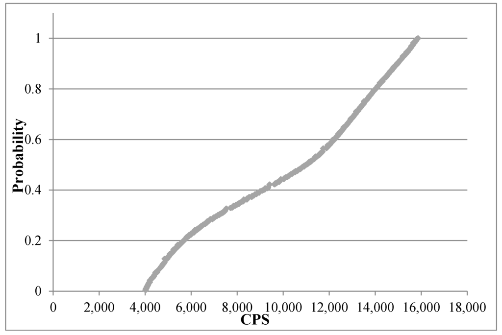
Figure 1. Cumulative Distribution Function: CPS (Million USD).

Figure 1. Cumulative Distribution Function: CPS (Million USD).

Our estimation of the welfare impact for the climate change scenario (USD 14.8 billion) lays in the upper part of the cumulative distribution, with a probability of occurrence higher than 80%, thus confirming the significance of the results obtained and their robustness in terms of sensitivity to climatic uncertainty. The analysis of the distribution shows also that the 50th percentile is USD 11 billion and the 25th percentile is USD 6.347 billion, thus indicating that even quite lower CPS values could be determined by climatic variability, but their probability of occurrence following our assumptions is rather low.

In a wider context, our results are in line with other studies, at both national and global scales, in which climate change could threaten the agricultural sector. At the national level, the results reported here are consistent with those reported by previous studies in Chile, with largest impacts on the northern zone and small aggregated impacts. According to our results, the impact on the total agricultural net income (−16%) is larger than the ones reported in previous studies. For the same climate change scenario (A2-2040) [38], reported the lower bound of −10% on income change, while [40] reported the upper bound (−3%). The gap between our results and previous ones is explained by the different methodologies used in each case. Even though our model explicitly includes the demand side, the modeling approach -using own price elasticity matrix- does not allow for substitution. On the other hand, at the global level, [57] found that climate change will drive an increase on both maize and wheat prices, with associated impacts on the meat market. Regarding the distributive impacts of climate change, [58] reported large distributional consequences across countries and activities due to climate change. Finally, there is an increasing discussion within the literature about the economic models’ assumptions about farmers’ adaptive capacity, in which most of the adaptation costs are ignored, overestimating their capacity to cope with climate change [59,60].

4. Conclusions

The main conclusion of this study is that the welfare effects of changes in water availability are small at the national level, but with considerable distributional effects. At activity level, plum, walnut, and avocado producers will be worse-off compared to vineyard, orange, and apple producers. This could worsen the inequity that already exists in Chile, presenting additional challenges for coping with climate change. On the other hand, the average decrease in demand prices of 1% within agricultural products hides large differences across sectors.

However, despite the modeling effort conducted in this research, some drawbacks remain. These limitations are related to the demand system, input substitution, and irrigation facilities. The way in which the demand system is modeled does not allow for the analysis of poverty issues that could be a consequence of changes in the agricultural sector’s production structure. Due to a lack of information, the model does not account for substitution options between water and other inputs, nor does it consider the use of irrigation deficits as an adaptation option to climate change. Then again, the model assumes that the expansion of the irrigated area is costless, underestimating the costs associated to the change in the crop pattern. Finally, climate change impacts on the rainfed sector are modeled as a productivity shock, without an explicit functional form relating water and agricultural yields. Nevertheless, the structure of the model allows us to include these topics once the data becomes available.

The re-allocation of land across the country implies several impacts that are not modeled here, such as: environmental impacts due to land use change, as well as social impacts. Regarding the latter, the use of these types of models should be part of a more complete analysis of climate change in the agricultural sector, these analyses should explicitly include the social component. This is very important considering the social consequences of changes in farming practices that are deeply rooted within the farmers’ communities.

References

- Stocker, T.F.; Qin, D.; Plattner, G.K.; Tignor, M.; Allen, S.K.; Boschung, J.; Nauels, A.; Xia, Y.; Bex, V.; Midgley, P.M. Climate change 2013: The physical science basis. In Contribution of Working Group I to the Fifth Assessment Report of the Intergovernmental Panel on Climate Change; Cambridge University Press: Cambridge, UK; New York, NY, USA, 2013; p. 1535. [Google Scholar]
- Bates, B.; Kundzewicz, Z.W.; Wu, S.; Palutikof, J. Climate Change and Water; Intergovernmental Panel on Climate Change (IPCC): Geneva, Switzerland, 2008. [Google Scholar]
- Field, C.B.; Barros, V.R.; Mach, K.; Mastrandrea, M. Climate change 2014: Impacts, adaptation, and vulnerability. In Contribution of Working Group II to the Fifth Assessment Report of the Intergovernmental Panel on Climate Change; Cambridge University Press: Cambridge, UK; New York, NY, USA, 2014. [Google Scholar]
- Fischer, G.; Shah, M.; Tubiello, F.N.; van Velhuizen, H. Socio-Economic and climate change impacts on agriculture: An integrated assessment, 1990–2080. Philos. Trans. R. Soc. B Biol. Sci. 2005, 360, 2067–2083. [Google Scholar] [CrossRef] [PubMed]
- Alcamo, J.; Flörke, M.; Märker, M. Future long-term changes in global water resources driven by socio-economic and climatic changes. Hydrol. Sci. J. 2007, 52, 247–275. [Google Scholar] [CrossRef]
- Arnell, N.W.; van Vuuren, D.P.; Isaac, M. The implications of climate policy for the impacts of climate change on global water resources. Glob. Environ. Chang. 2011, 21, 592–603. [Google Scholar] [CrossRef]
- Food and Agriculture Organization of the United Nations (FAO). Statistical Yearbook; FAO: Rome, Italy, 2013. [Google Scholar]
- Van Vuuren, D.P.; Edmonds, J.; Kainuma, M.; Riahi, K.; Thomson, A.; Hibbard, K.; Hurtt, G.C.; Kram, T.; Krey, V.; Lamarque, J.F. The representative concentration pathways: An overview. Clim. Chang. 2011, 109, 5–31. [Google Scholar] [CrossRef]
- Wheeler, T.; von Braun, J. Climate change impacts on global food security. Science 2013, 341, 508–513. [Google Scholar] [CrossRef] [PubMed]
- Dowlatabadi, H. Integrated assessment models of climate change: An incomplete overview. Energy Policy 1995, 23, 289–296. [Google Scholar] [CrossRef]
- Weyant, J.P. General economic equilibrium as a unifying concept in energy-economic modeling. Manag. Sci. 1985, 31, 548–563. [Google Scholar] [CrossRef]
- Hazell, P.B.; Norton, R.D.; Hazell, P.B.R.; Hazell, P.B.R. Mathematical Programming for Economic Analysis in Agriculture; Macmillan: New York, NY, USA, 1986. [Google Scholar]
- Sadoulet, E.; de Janvry, A. Quantitative Development Policy Analysis; Johns Hopkins University Press: Baltimore, MD, USA, 1995. [Google Scholar]
- Howitt, R.E. Agricultural and Environmental Policy Models: Calibration, Estimation and Optimization. Davis: University of California, Davis. Available online: http://www.infoandina.org/sites/default/files/publication/files/Howitt_DraftBook.pdf (accessed on 9 May 2015).
- Croppenstedt, A.; Bellú, L.G.; Bresciani, F.; DiGiuseppe, S. Agricultural Policy Impact Analysis with Multi-Market Models: A Primer; Agricultural Development Economics Division (ESA): Rome, Italy, 2007. [Google Scholar]
- Arulpragasam, J.; Conway, P. Partial equilibrium multi-market analysis. In The Impact Of Economic Policies on Poverty and Income Distribution Evaluation Techniques and Tools; The World Bank and Oxford University Press: Washington, DC, USA, 2003; pp. 261–277. [Google Scholar]
- Rich, K.; Lundberg, M. Multimarket Models and Policy Analysis: An Application to Madagascar; The World Bank Group: Washington, DC, USA, 2002. [Google Scholar]
- Norton, R.D.; Solís, L. The Book of Chac Programming Studies for Mexican Agriculture; The World Bank: Washington, DC, USA, 1983. [Google Scholar]
- Stifel, D.; Randrianarisoa, J.C. Rice Prices, Agricultural Input Subsidies, Transaction Costs and Seasonality: A Multi-Market Model Poverty and Social Impact Analysis (Psia) for Madagascar; World Bank: Washington, DC, USA, 2004. [Google Scholar]
- Siam, G.M.; Croppenstedt, A. An assessment of the Impact of Wheat Market Liberalization in Egypt: A Multi Market Model Approach; Agricultural Development Economics Division (ESA): Rome, Italy, 2007. [Google Scholar]
- Van Ittersum, M.K.; Ewert, F.; Heckelei, T.; Wery, J.; Olsson, J.A.; Andersen, E.; Bezlepkina, I.; Brouwer, F.; Donatelli, M.; Flichman, G. Integrated assessment of agricultural systems—A component-based framework for the European Union (seamless). Agric. Syst. 2008, 96, 150–165. [Google Scholar] [CrossRef]
- Britz, W.; Witzke, P. Capri Model Documentation 2008: Version 2; Institute for Food and Resource Economics, University of Bonn: Bonn, Germany, 2008. [Google Scholar]
- Schneider, U.A.; Balkovic, J.; de Cara, S.; Franklin, O.; Fritz, S.; Havlik, P.; Huck, I.; Jantke, K.; Kallio, A.M.I.; Kraxner, F. The European Forest and Agricultural Sector Optimization Model–Eufasom; FNU-156; Hamburg University and Centre for Marine and Atmospheric Science: Hamburg, Germany, 2008. [Google Scholar]
- Rosegrant, M.W.; Msangi, S.; Ringler, C.; Sulser, T.B.; Zhu, T.; Cline, S.A. International Model for Policy Analysis of Agricultural Commodities and Trade (Impact): Model Description; International Food Policy Research Institute: Washington, DC, USA, 2008. [Google Scholar]
- Adams, D.M.; Alig, R.J.; Callaway, J.M.; McCarl, B.A.; Winnett, S.M. The Forest and Agricultural Sector Optimization Model (Fasom): Model Structure and Policy Applications; DIANE Publishing: Portland, OR, USA, 1996. [Google Scholar]
- Lehtonen, H.; Aakkula, J.; Rikkonen, P. Alternative agricultural policy scenarios, sector modelling and indicators: A sustainability assessment. J. Sustain. Agric. 2005, 26, 63–93. [Google Scholar] [CrossRef]
- Helming, J.; Reinhard, S. Modelling the economic consequences of the eu water framework directive for Dutch agriculture. J. Environ. Manag. 2009, 91, 114–123. [Google Scholar] [CrossRef] [PubMed]
- Alabdulkader, A.M.; Al-Amoud, A.I.; Awad, F.S. Optimization of the cropping pattern in Saudi Arabia using a mathematical programming sector model. Agric. Econ. (Zemědělská Ekon.) 2012, 58, 56–60. [Google Scholar]
- Helming, J.; Peerlings, J. Economic and environmental effects of a flat rate for Dutch agriculture. NJAS Wagening. J. Life Sci. 2014, 68, 53–60. [Google Scholar] [CrossRef]
- Deppermann, A.; Grethe, H.; Offermann, F. Distributional effects of cap liberalisation on western german farm incomes: An ex-ante analysis. Eur. Rev. Agric. Econ. 2014, 41, 605–626. [Google Scholar] [CrossRef]
- Pattanayak, S.K.; McCarl, B.A.; Sommer, A.J.; Murray, B.C.; Bondelid, T.; Gillig, D.; DeAngelo, B. Water quality co-effects of greenhouse gas mitigation in US agriculture. Clim. Chang. 2005, 71, 341–372. [Google Scholar] [CrossRef]
- Schneider, U.A.; McCarl, B.A.; Schmid, E. Agricultural sector analysis on greenhouse gas mitigation in us agriculture and forestry. Agric. Syst. 2007, 94, 128–140. [Google Scholar] [CrossRef]
- Pedercini, M.; Kanamaru, H.; Derwisch, S. Potential Impacts of Climate Change on Food Security in Mali; Food and Agriculture Organization of the United Nations (FAO): Rome, Italy, 2012. [Google Scholar]
- Shakhramanyan, N.G.; Schneider, U.A.; McCarl, B.A. Us agricultural sector analysis on pesticide externalities—The impact of climate change and a pigovian tax. Clim. Chang. 2013, 117, 711–723. [Google Scholar] [CrossRef]
- McCarl, B.A.; Musumba, M.; Smith, J.B.; Kirshen, P.; Jones, R.; El-Ganzori, A.; Ali, M.A.; Kotb, M.; el-Shinnawy, I.; el-Agizy, M. Climate change vulnerability and adaptation strategies in Egypt’s agricultural sector. Mitig. Adapt. Strateg. Glob. Chang. 2013. [Google Scholar] [CrossRef]
- González, J.; Velasco, R. Evaluation of the impact of climatic change on the economic value of land in agricultural systems in chile. Chil. J. Agric. Res. 2008, 68, 56–68. [Google Scholar] [CrossRef]
- Mendelsohn, R.; Nordhaus, W.D.; Shaw, D. The impact of global warming on agriculture: A ricardian analysis. Am. Econ. Rev. 1994, 753–771. [Google Scholar]
- Samaniego, J.; de Miguel, C.J.; Galindo, L.M.; Gómez, J.J.; Martínez, K.; Cetrángolo, O. La economía del cambio climático en chile: Síntesis; Economic Commission for Latin America and the Caribbean (CEPAL): Santiago, Chile, 2009. (In Spanish) [Google Scholar]
- Oficina de Estudios y Políticas Agrarias (ODEPA). Estimación del Impacto Socioeconómico del Cambio Climático en el Sector Silvoagropecuario de Chile; ODEPA: Santiago, Chile, 2010. (In Spanish) [Google Scholar]
- Ponce, R.; Blanco, M.; Giupponi, C. The economic impacts of climate change on the chilean agricultural sector: A non-linear agricultural supply model. Chil. J. Agric. Res. 2014, 74, 404–412. [Google Scholar] [CrossRef]
- Howitt, R.E. Positive mathematical programming. Am. J. Agric. Econ. 1995, 77, 329–342. [Google Scholar] [CrossRef]
- Havlík, P.; Schneider, U.A.; Schmid, E.; Böttcher, H.; Fritz, S.; Skalský, R.; Aoki, K.; de Cara, S.; Kindermann, G.; Kraxner, F. Global land-use implications of first and second generation biofuel targets. Energy Policy 2011, 39, 5690–5702. [Google Scholar] [CrossRef]
- Chang, C.C.; McCarl, B. Scope of ASM: The US Agricultural Sector Model; Draft Report; Texas A & M University: College Station, TX, USA, 1990. [Google Scholar]
- Heckelei, T. Calibration and Estimation of Programming Models for Agricultural Supply Analysis; University of Bonn: Bonn, Germany, 2002. [Google Scholar]
- Blanco, M.; Cortignani, R.; Severini, S. Evaluating changes in cropping patterns due to the 2003 cap reform. An ex-post analysis of different pmp approaches considering new activities. In Proceedings of the 107th Seminar of the European Association of Agricultural Economists, Sevilla, Spain, 30 January–1 February 2008.
- Howitt, R.; Medellin-Azuara, J.; MacEwan, D. Estimating the Economic Impacts of Agricultural Yield Related Changes for California; California Climate Change Center: Sacramento, CA, USA, 2009; Volume Vloume 19, pp. 16–17. [Google Scholar]
- Howitt, R.E.; MacEwan, D.; Medellín-Azuara, J.; Lund, J.R. Economic Modeling of Agriculture and Water in California Using the Statewide Agricultural Production Model; University of California: Davis, CA, USA, 2010. [Google Scholar]
- De Frahan, B.H.; Buysse, J.; Polomé, P.; Fernagut, B.; Harmignie, O.; Lauwers, L.; Van Huylenbroeck, G.; van Meensel, J. Positive mathematical programming for agricultural and environmental policy analysis: Review and practice. In Handbook of Operations Research in Natural Resources; Springer: New York, NY, USA, 2007; pp. 129–154. [Google Scholar]
- Heckelei, T.; Britz, W.; Zhang, S. Positive mathematical programming approaches—Recent developments in literature and applied modelling. Bio-Based Appl. Econ. 2012, 1, 109–124. [Google Scholar]
- Hardaker, J.B.; Huirne, R.B.; Anderson, J.R.; Lien, G. Coping with Risk in Agriculture; CABI Publishing: Cambridge, MA, USA, 2004. [Google Scholar]
- Instituto Nacional de Estadísticas (INE). Censo Agropecuario y Forestal; INE: Santiago, Chile, 2007. (In Spanish)
- The World Bank. Data Catalog. Available online: http://data.worldbank.org/ (accessed on 18 April 2014).
- Oficina de Estudios y Políticas Agrarias (ODEPA). Available online: http://www.odepa.cl (accessed on 5 March 2014). (In Spanish)
- Quiroz, J.; Labán, R.; Larraín, F. El Sector Agrícola y Agroindustrial Frente a Nafta y Mercosur; Sociedad Nacional de Agricultura: Santiago, Chile, 1995; p. 149. (In Spanish) [Google Scholar]
- Foster, W.; López de Lérida, J.; Valdes, A. Impacto del Nivel de Distorsiones en el Sector Agrícola Nacional; Ministerio de Agricultura: Santiago, Chile, 2011. (In Spanish) [Google Scholar]
- Santibáñez, F.; Santibáñez, P.; Cabrera, R.; Solís, L.; Quiroz, M.; Hernández, J. Análisis de Vulnerabilidad del Sector Silvoagropecuario, Recursos Hídricos, Edáficos de Chile Frente a Escenarios de Cambio Climático; Centro de Agricultura y Medioambiente (AGRIMED): Santiago, Chile, 2008. (In Spanish) [Google Scholar]
- Nelson, G.C.; Rosegrant, M.W.; Koo, J.; Robertson, R.; Sulser, T.; Zhu, T.; Ringler, C.; Msangi, S.; Palazzo, A.; Batka, M. Climate Change: Impact on Agriculture and Costs of Adaptation; International Food Policy Research Institute: Washington, DC, USA, 2009; Volume 21. [Google Scholar]
- Arent, D.; Tol, R.; Faust, E.; Hella, J.; Kumar, S. Key economic sectors and services. In Climate Change 2014: IMPACTS, Adaptation, and Vulnerability. Part A: Global and Sectoral Aspects. Contribution of Working Group II to the Fifth Assessment Report of the Intergovernmental Panel on Climate Change; Cambridge University Press: Cambridge, UK; New York, NY, USA, 2014; pp. 659–708. [Google Scholar]
- Nelson, G.C.; Valin, H.; Sands, R.D.; Havlík, P.; Ahammad, H.; Deryng, D.; Elliott, J.; Fujimori, S.; Hasegawa, T.; Heyhoe, E. Climate change effects on agriculture: Economic responses to biophysical shocks. Proc. Natl. Acad. Sci. USA 2014, 111, 3274–3279. [Google Scholar] [CrossRef] [PubMed]
- Antle, J. Agriculture and the Food System: Adaptation to Climate Change; Resources for the Future: Washington, DC, USA, 2009. [Google Scholar]
© 2015 by the authors; licensee MDPI, Basel, Switzerland. This article is an open access article distributed under the terms and conditions of the Creative Commons Attribution license (http://creativecommons.org/licenses/by/4.0/).