Article

Determining Characteristic Vegetation Areas by Terrestrial Laser Scanning for Floodplain Flow Modeling

1
Department of Civil and Environmental Engineering, Aalto University, P.O. Box 15500, Aalto 00076, Finland
2
Department of Real Estate, Planning and Geoinformatics, Aalto University, P.O. Box 15800, Aalto 00076, Finland
*
Author to whom correspondence should be addressed.
Water 2015, 7(2), 420-437; https://doi.org/10.3390/w7020420
Submission received: 26 November 2014 / Revised: 13 January 2015 / Accepted: 21 January 2015 / Published: 29 January 2015
(This article belongs to the Special Issue Advances in Remote Sensing of Flooding)

Abstract

:
Detailed modeling of floodplain flows and associated processes requires data on mixed, heterogeneous vegetation at river reach scale, though the collection of vegetation data is typically limited in resolution or lack spatial information. This study investigates physically-based characterization of mixed floodplain vegetation by means of terrestrial laser scanning (TLS). The work aimed at developing an approach for deriving the characteristic reference areas of herbaceous and foliated woody vegetation, and estimating the vertical distribution of woody vegetation. Detailed experimental data on vegetation properties were gathered both in a floodplain site for herbaceous vegetation, and under laboratory conditions for 2–3 m tall trees. The total plant area (Atot) of woody vegetation correlated linearly with the TLS-based voxel count, whereas the Atot of herbaceous vegetation showed a linear correlation with TLS-based vegetation mean height. For woody vegetation, 1 cm voxel size was found suitable for estimating both the Atot and its vertical distribution. A new concept was proposed for deriving Atot for larger areas from the point cloud attributes of small sub-areas. The results indicated that the relationships between the TLS attributes and Atot of the sub-areas can be derived either by mm resolution TLS or by manual vegetation sampling.

Graphical Abstract

1. Introduction

Vegetation influences flow of water in rivers and floodplains with implications on many physical, chemical, and biological processes (e.g., [1,2]). In the context of flood flow analyses, vegetation is a critical factor in determining hydraulic resistance and water levels [3,4,5]. Generally, flow-vegetation interactions affect sediment and solute transport, channel morphology, and habitat quality. In environmentally sensitive engineering practices, vegetation is used for riverbank stabilization, increasing biodiversity, and forming riparian buffer zones, where the monitoring of vegetation structure and diversity is essential for improving future practices [6]. For the monitoring and modeling of riverine environments and floodplain flows, vegetation characteristics describing the structure and distribution of vegetation are needed. Physically-based parameterization of complex natural vegetation is essential in developing reliable hydro-environmental models [3].
Conventional hydraulic modeling applications are typically based on calibrated values of resistance coefficients such as Manning’s n or Darcy–Weisbach f, or on values from similar reference sites, e.g., [1]. Many models simplify natural vegetation to cylindrical elements (see [3]). For such cylinders, the drag force (F) resulting from viscous and pressure drag can be parameterized by
F = 1 2 ρ C D A C U 2
where, ρ = fluid density; CD = drag coefficient; AC = characteristic plant area; and U = reference velocity. AC is often defined as the frontal projected area AP (bl, where b = width and l = height), and the CD depends on the Reynolds number. In estimating resistance coefficients and water levels, vegetation is often assumed to be linearly distributed over the height [3]. For complex shaped natural flexible vegetation, the approximations derived for cylinders are inadequate, as plants reconfigure in a flow (i.e., change their shape due to streamlining and bending).
Modern research recommends the use of leaf and stem (including branches) areas as characteristic reference area properties for flow resistance estimations [7,8,9]. Furthermore, the characteristic plant area over height needs to be correctly estimated to account for the impact of the vertical vegetation structure on the flow resistance for different stages of submersion [10]. To diminish calibration, recent studies on modeling vegetated flows have focused on physically-based parameterization of woody [7,9,11,12] and aquatic [13,14,15,16] vegetation. The area occupied by vegetation plays a key role in the estimates, and various area-based parameterizations are presented for different types of vegetation: the leaf area index (LAI) [9,17,18], the total area of the trees (Atot) [11], the cross-sectional blockage factor [13,15], and the frontal area per unit volume (AC/V) [19].
Conventional ground-based monitoring of vegetation characteristics is time-demanding and laborious. Remote sensing methods exist to derive floodplain hydraulic roughness from satellites (digital and radar imagery) or from airborne platforms (LiDAR and orto-photography) [20,21]. Laser scanning (LS) provides a means to derive the spatially explicit horizontal and vertical distribution of vegetation characteristics applied in the flow models. LS gathers three-dimensional (3D) information about objects, and is widely adopted in the monitoring of built and natural environments. The 3D LS point clouds allow for estimating the total vegetation area in contrast to photographic analyses, which estimate the frontal projected area. In hydraulic analyses the total area is important, as all of the leaves and branches contribute to the resistance and the shaded plant parts behind the frontal area should also be accounted for [9]. Moreover, photographic analyses overestimate the portion of vegetation closer to the camera due to the central projection on the image [22].
LS is employed in terrestrial (TLS), airborne (ALS) and mobile (MLS) platforms. In MLS the scanner can be mounted on a car, boat or backpack [23]. The resolution and accuracy of LS measurements depend on the scanner and its distance to the object, and the platform. Large areas are often surveyed with ALS or MLS, whereas TLS is commonly applied in small-scale analyses in estimating riverbed morphology, roughness, and river bank retreat with as high as grain-scale accuracy [24,25,26,27,28] and in detecting centimeter-resolution bathymetry in gravel bed rivers in clear and shallow waters [29]. To reduce occlusion and to cover larger areas, TLS point clouds are produced from multiple sub-scans [30]. The occlusion effects can be decreased further by combining measurements conducted from different platforms and by combining them with TLS from multiple scan stations [20,23,31,32].
TLS has been proved to be a suitable tool for the estimation of vegetation density from the number of points passing through a 3D voxel and from the points intercepted in the voxel [22,33]. A voxel refers to a data point or a cell in a regularly spaced, three-dimensional grid. Leaf area can be analyzed from voxelization of the point clouds [34,35], and the vertical leaf area distribution by the optical laser point-quadrate method [36] and by the gap fraction and the Beer–Lambert law [37]. Many of the methods are derived for trees, and the properties of a varying floodplain cover of bushy and grassy type of vegetation are less explored. Such mixed low vegetation is often considered in LS applications a factor to be eliminated from the data as it complicates the ground detection [38], but for hydraulic modeling applications, detecting detailed information about the vegetation and its distribution is essential.
It is evident that for estimating physically-based and spatially accurate vegetation characteristics for hydro-environmental modeling applications, methods are needed for analyzing registered multi-station or multi-platform point clouds. Consequently, this paper investigates the estimation of the characteristic reference areas of mixed floodplain vegetation by employing multi-station TLS both in field and laboratory conditions. Specifically, the work aimed at developing a practice-oriented approach (1) to derive the total plant areas of herbaceous vegetation and foliated woody vegetation; and (2) to estimate the vertical distribution of the total plant area of foliated woody vegetation for different levels of submergence.

2. Methods

Terrestrial laser scanning of herbaceous vegetation was conducted at a field site, where vegetation samples were collected from quadrates of 1 m2 in size (Section 2.1). For obtaining characteristics of woody vegetation (Section 2.2), TLS of trees was conducted in laboratory conditions in connection with an experimental investigation on hydraulic resistance of woody vegetation [11] (Section 2.2). Regressions between attributes of TLS-based point cloud and characteristic vegetation areas were derived for woody and herbaceous vegetation (Section 2.3). These regressions were tested against independent field data from a TLS campaign conducted two years earlier (Section 2.3).

2.1. Herbaceous Vegetation: TLS Campaign and Manual Vegetation Sampling in the Field

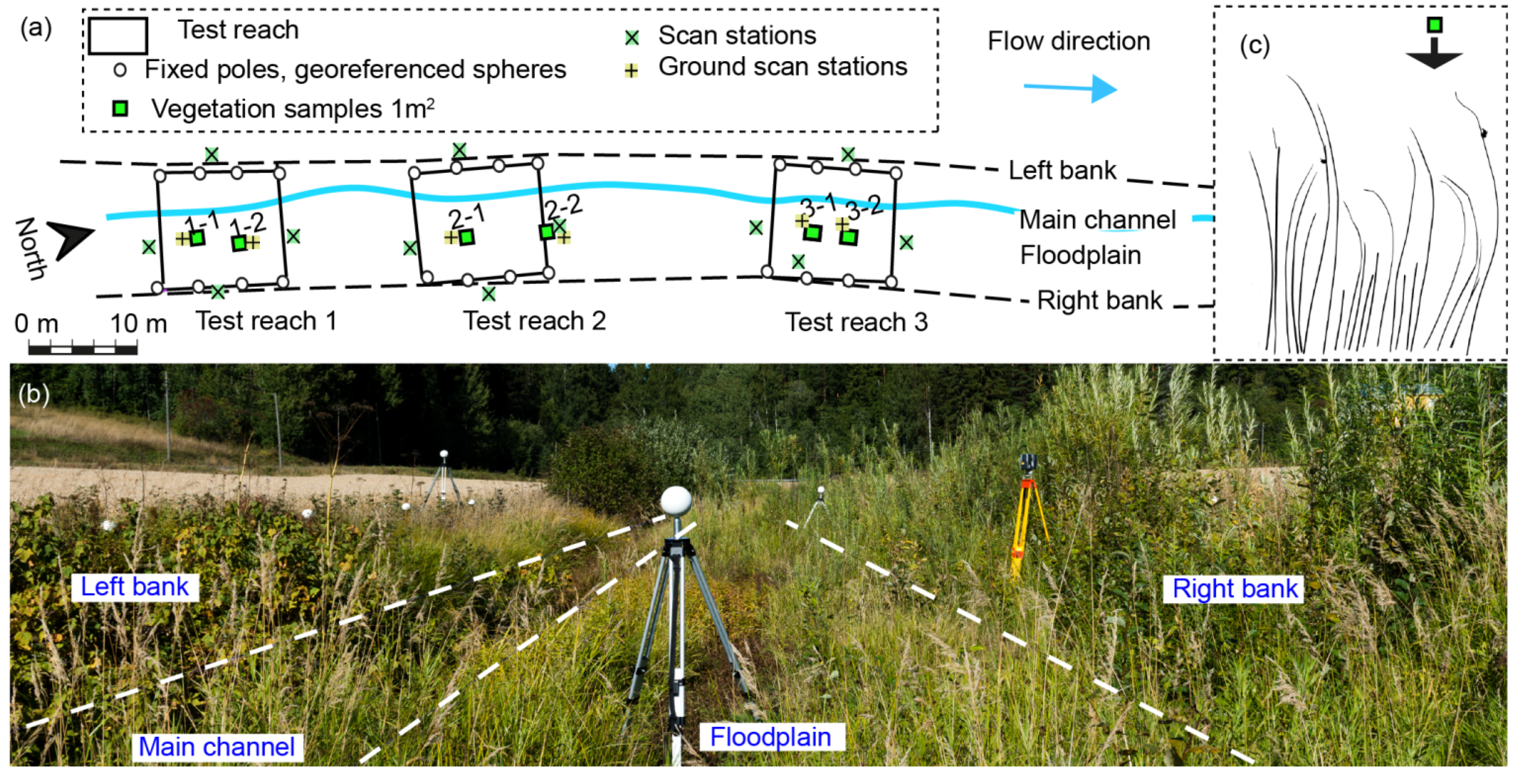
The field investigations were conducted in a 200 m long two-stage channel having 20 m long test reaches of different floodplain vegetation in Sipoo in southern Finland [39]. The two-stage channel had a bankful width of 11 m, where the width of the floodplain was 4–6 m. The site was laser scanned in August 2013 (Figure 1 and Figure 2) with Faro Focus 3D scanner (FARO Technologies, Lake Mary, FL, USA) which has a 305° × 360° field of view, a range up to 153 m, a scan rate up to 976,000 points/sec, and beam divergence of 0.19 mrad. The scanning resolution used produced a point spacing of 6 mm at a distance of 10 m. Three test reaches were scanned from multiple locations (from both of the banks and the floodplain) after which vegetation samples were collected by harvesting the vegetation from two 1 m2 sampling quadrates of each test reach (Figure 1 and Figure 2). To obtain ground level, the quadrates were scanned after the removal of vegetation, and the DTM of the sampling quadrates was obtained from the scan by selecting the lowest elevations in a 1 cm grid. The point clouds were registered using georeferenced spherical targets located at the channel banks (Figure 2). The stray points were filtered with a statistical outlier removal filter (SOR, [40]) in CloudCompare, which computes the mean distance for each point. The resulted points whose mean distances are outside an interval defined by the global distances mean and standard deviation are considered as outliers and removed from the data. The number of points used for the mean distance estimation was ten and the standard deviation multiplier threshold was one.
Figure 1. Field campaign: Acquisition of the point clouds and manual vegetation samples.
Water 07 00420 g001
The vegetation cover consisted mostly of different types of grassy plants with occasional small (≈1 m) willows, birches and lupines amidst. The sampling quadrates were selected to represent grassy herbaceous vegetation (i.e., not woody or bushy vegetation). From the vegetation samples of the quadrates, the dry and wet mass, and volume were analyzed in laboratory. To obtain the total plant area (Atot), the vegetation samples were photographed against a white background. Due to the large sampling size, the vegetation from a sampling quadrate was divided to several small samples photographed individually (Figure 2c). The total plant area (Atot) was obtained from the photographs by counting the pixels representing vegetation. The scale was obtained from a ruler placed at the sides of the white background. The total plant area per ground area (Atot/AB) was obtained from the sum of the vegetation in the photographs divided by the ground area of the sampling quadrate (1 m2).
Figure 2. Field campaign: (a) locations of the scanner and vegetation sampling quadrates; (b) the TLS campaign at the reach in dry conditions; and (c) example of sampled vegetation photographed for the estimation of Atot.
Water 07 00420 g002
TLS campaigns at the field site were conducted in November 2011 and after snowmelt in May 2012 (see [30]), and these independent datasets are used in the testing procedure of the TLS characteristic area analyses described below. The manual samples of the grassy test reaches were collected from the test reaches from 5 to 6 sampling quadrates of 12.5 × 12.5 cm2 in size by [30,39]. The vegetation samples were photographed against a white canvas with a scale adjusted to the side, and the Atot was estimated by counting the pixels representing vegetation [30]. The samples were taken from randomly selected quadrates to obtain test reach averaged plant area, and thus the exact sampling locations were not recorded. The willow samples were collected from a quadrate of 1.12 × 1.12 m2 by [39]. Three test reaches were used in the testing process: grasses in the upstream part of the reach (Grasses-U, mean height Hm = 0.5 m), grasses in the downstream part (Grasses-D, Hm = 0.4 m) and willow vegetated test reach with cut grasses (Willows-M, ≈1 m tall). The May 2012 data (TLS after snowmelt) was used to create a DTM of the ground topography for the independent test data.

2.2. Woody Vegetation: TLS and Manual Measurements of Trees in the Laboratory

Three foliated Alnus glutinosa (Common Alder, AG) and Salix caprea (Goat Willow, SC) specimens of 1.8–3.4 m in height were laser scanned in a laboratory. The specimens were taken from a wetland area in Espoo, southern Finland in the beginning of June when vegetation had reached full foliage [11]. The LS was conducted at 3–4 m distance of the object from three directions with Leica ScanStation C10 (Leica Geosystems AG, Heerbrugg, Switzerland). The ScanStation C10 has a 360° × 270° field of view, a range up to 300 m, a scan rate up to 50,000 points/s, and 4 mm spot size (at a distance of 0–50 m). The scanning resolution was set to 5 mm at a distance of 10 m. The laser pulse follows a spherical geometry, and thus the resolution is higher closer to the scanner than at long distances. The individual scans were co-registered in Leica’s Cyclone software using spherical targets, and the segments from the scan area around the tree were manually removed from the point cloud. The co-registration error was 0–2 mm. Prior to the analyses, the incorrect points were filtered with SOR [40] (see Section 2.1). Fifty points were used for the mean distance estimation and the standard deviation multiplier threshold was one. These stray points were caused by the point size of the laser, and error points appeared e.g., from the edges of leaves.
The surface areas of the tree stems were obtained from manual measurements by recording the diameter and length of each of the branches and main stem in 20 cm segments assuming that the stems and branches were cylindrical elements (see [41]). Consequently, AS was defined as half of the circular stem area, which represents the area exposed to the flow attack. The leaf areas were obtained by scanning the leaves with a flatbed document scanner. Due to the large size of the trees, the total leaf area was estimated using the specific leaf area, which is the leaf area to dry mass ratio (SLA = AL/md,L, commonly used for estimating the leaf area index [42]). For the leaf dry mass (md,L) and leaf area analyses, the trees were divided into four height sections (quartiles). For the second highest section of a specimen, three samples were taken and the SLA was determined for each of them. To guarantee the accuracy of SLA, the results of the three samples were compared. The differences between the SLA of a sample and the average of three varied between 0% and 6%. The dry mass (md) was estimated for all the four height quartiles, and the SLA was used to obtain the AL of each quartile [11]. The total plant area of the tree (Atot) was estimated as the sum of the manually measured AL and AS.

2.3. Characteristic Reference Areas: Regressions between TLS-Based Point Cloud Attributes and Total Plant Area
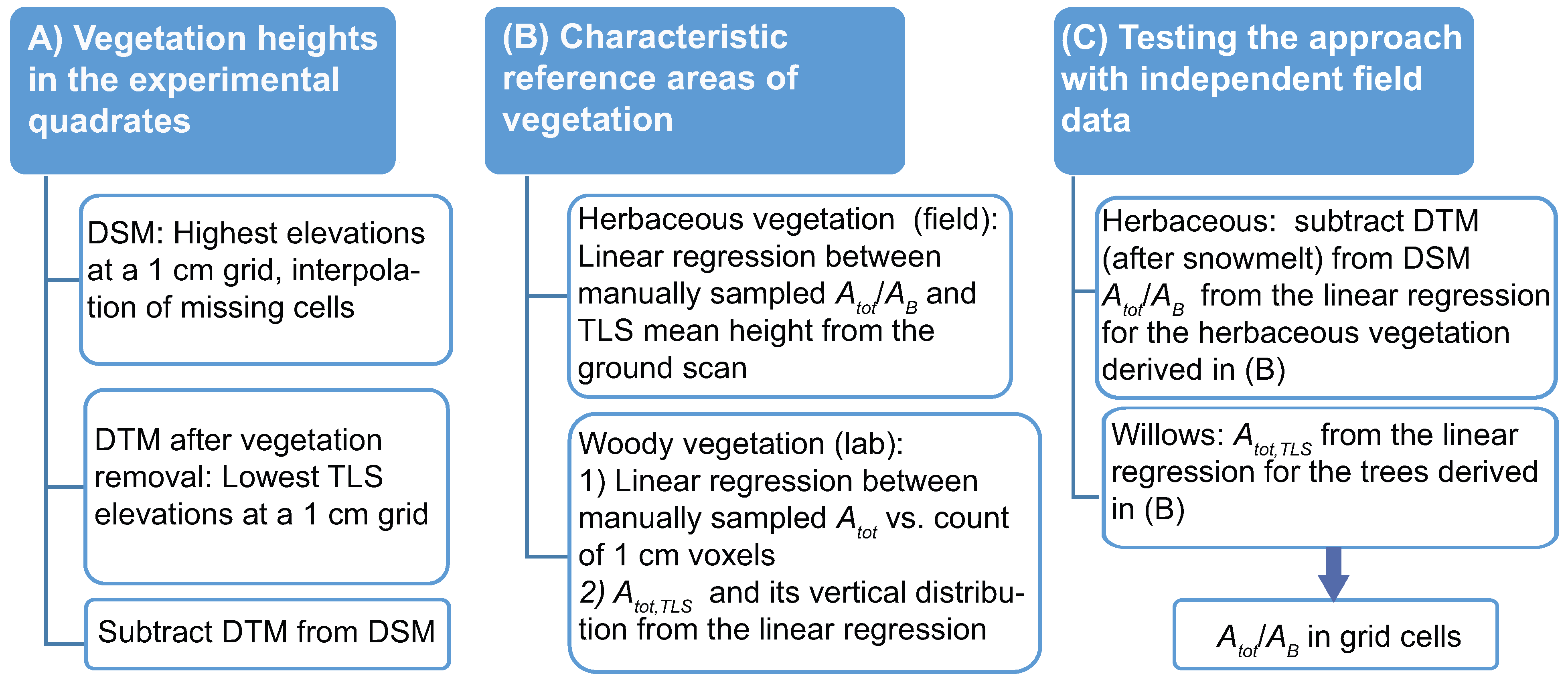
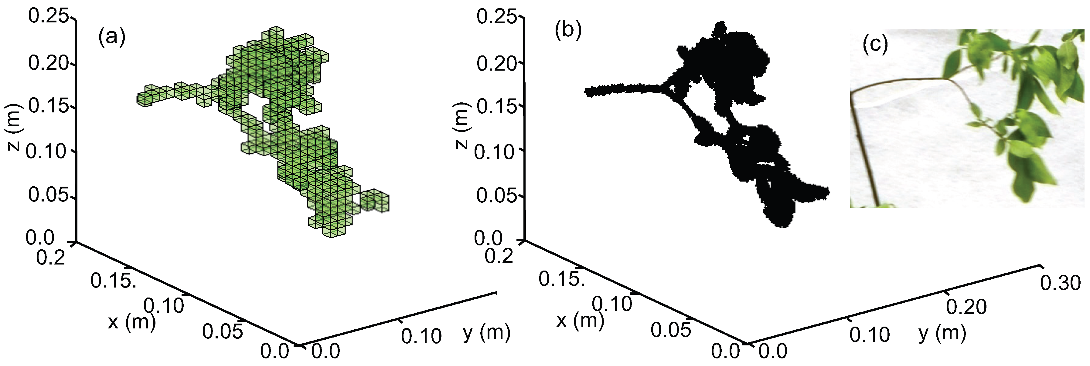
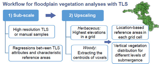
The process of obtaining the TLS-based characteristic reference areas for the herbaceous and woody vegetation is described in Figure 3. For woody vegetation, the linear regression between the count of voxels and manually sampled total area was derived for the trees in laboratory. The voxel sizes of 1 cm, 5 cm, and 10 cm were investigated. The point cloud was subsampled by a minimum distance of 1 cm, 5 cm and 10 cm between the points and sampled to a voxel grid with the centroids of the voxels recorded using CloudCompare 2.5.4.1 (GPL software, EDF R&D, Telecom ParisTech, Paris, France) and Matlab R2014a (The MathWorks, Inc., Natick, MA, USA) (Figure 4). The vertical distribution (Az) of the total plant area of trees was obtained from the linear regression of Atot vs. voxel count, and the differences between the manual samples of the quartiles and Az,TLS were determined. For herbaceous vegetation a digital surface model (DSM) was created by selecting the highest elevations at 1 cm and 5 cm grids in ArcGIS 10.2.2 (ESRI, Redlands, CA, USA) and by interpolating the missing values with natural neighbor interpolation. To obtain vegetation heights, the DTM of the quadrates after vegetation removal was subtracted from the DSM and the mean heights were estimated from the resulting height map. A linear regression between the vegetation mean height and total plant area was derived for the 1 m2 quadrates.
Figure 3. The process of deriving the characteristic reference areas for herbaceous and woody vegetation in the field and laboratory investigations.
Water 07 00420 g003
Figure 4. A voxelized branch of a S. caprea specimen (SC3) with (a) 1 cm voxel size and (b) 1 mm voxel size and (c) a photograph of the branch (note slightly different angle of view).
Water 07 00420 g004
The independent point cloud data from November 2011 [30] were used to test the linear regressions (Figure 3) for three test reaches: one with planted willows of Salix viminalis (Willows-M), and two grassy reaches (Grasses-D and -U). The DTM for the test reaches was obtained from a scan after snowmelt in May 2012 [30]. The vegetation points from November 2011 were classified with Canupo tools ([27]). Canupo classifies point clouds according to the geometrical shape of the point cloud. The classifier was trained using selected sections representing grasses and ground. Consequently, a classifier identifying willows was created for the Willows-M. The classification accuracy [27] of the vegetation was estimated from the number of points truly (t)/falsely (f) classified into the vegetation (v)/ground (g) classes, as a v = t v t v + f g . Similarly to the quadrates, the highest elevations were selected for the Grasses-D and -U, and the gaps were filled with the natural neighbor interpolation. To obtain the voxel count for the willows of the field site, the same workflow as for the laboratory specimens was carried out. The centroids of the voxels were determined and a raster map was generated containing the number of voxels for each raster cell, which allowed for estimating the Atot/AB from the relationship between the total number of the voxels and Atot.

3. Results and Discussion

3.1. Woody Vegetation
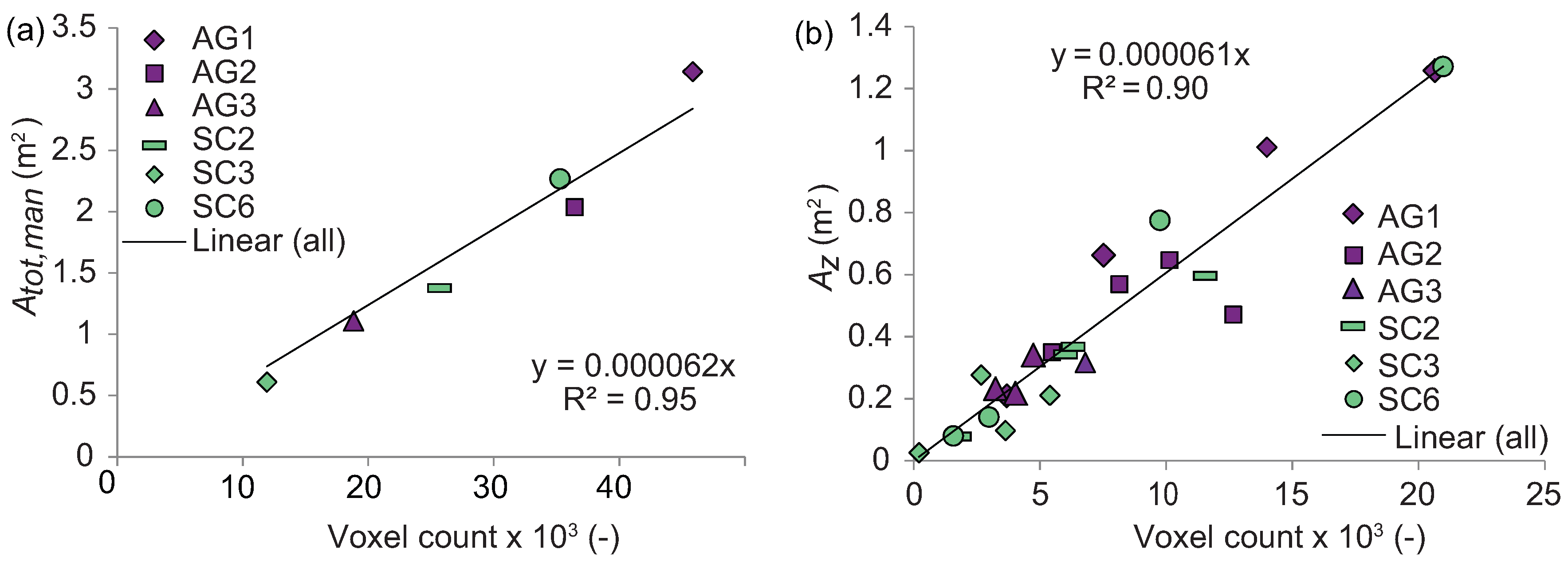
In deriving the total tree areas, a linear relationship was found between the manually measured Atot and TLS voxel count (Nvox) (Figure 5). The linear regression intercept was constrained to zero, resulting in Atot = 0.000062Nvox with R2 = 0.95 (Figure 5a). The Pearson correlation between the manually measured Atot and Nvox was statistically significant (0.98, p < 0.01). A similar R2 value was obtained using 5 cm (Atot = 0.0015Nvox, R2 = 0.948) and 10 cm (Atot = 0.0056Nvox, R2 = 0.914) voxels. The linear regressions depend on the point spacing, and thus prior to the voxel count the point clouds need to be subsampled (for large trees, lower resolution is adequate).
Figure 5. Manually measured Atot of the A. glutinosa and S. caprea specimens as a function of the count of 1 cm voxels for (a) all trees and (b) the same data divided to vertical quartiles.
Water 07 00420 g005
The linear fit using 1 cm voxels is shown for four vertical quartiles, Az, divided evenly over the specimen height in Figure 5b. The correlation between the vertical areas, Az, and Nvox was significant (0.95, p < 0.01) and the R2 was similar to the linear regression of the total plant area, although deviation from the mean was higher (Figure 5b). The Atot vs. Nvox values of the investigated S. caprea (SC) and A. glutinosa (AG) specimens were close to each other, and thus the linear regression was estimated for the two investigated species combined in Figure 5. This was justified, as the linear regression for the vertical quartiles with more data points (Figure 5b) showed comparable linear regression for the two species. However, it is expected that the linear regressions vary for different species due to interspecies variability in tree morphology.
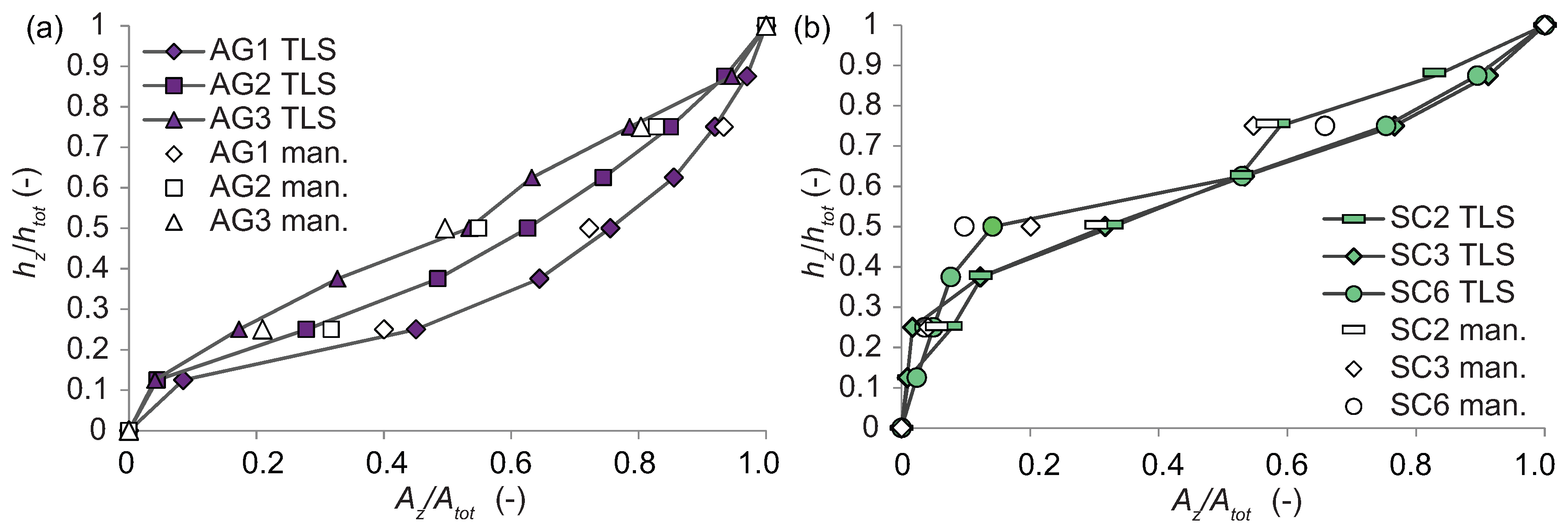
The difference to the manual measurements in the vertical quartiles estimated with the linear regression was 11% (Az,TLS larger than Az,man), while absolute difference was 28% (Figure 6). The estimation of the height sections with the manual sampling deviated slightly from the TLS height estimate, which may be a source of the larger deviation from the mean for the Az than Atot in comparison to manual sampling (Figure 5 and Figure 6). The vertical distribution of the total plant area deviated largely from a linear increase of area over height, particularly for the specimens of S. caprea (Figure 6b). This observation was in accordance with studies of vertical projected areas, where the cumulative projected areas, AP, deviated from a linear relationship over height assumed in cylinder based analyses [3].
Figure 6. Cumulative vertical distribution of the total plant area from TLS and manual sampling for the three specimens of (a) A. glutinosa and (b) S. caprea. The open symbols denote the manual measurements, and the colored symbols denote the TLS measurements with 1 cm voxels.
Water 07 00420 g006
The TLS analyses showed a difference in the plant structure between the specimens of the two species; the plant area of S. caprea was concentrated on the upper parts of the tree (Az/Atot ≈ 0.1 at hz/htot = 0.4, Figure 6b) whereas the plant area of A. glutinosa was concentrated on the lower parts of the tree (Az/Atot ≈ 0.5 at hz/htot = 0.4, Figure 6a). The different vertical distributions of the A. glutinosa and S. caprea species (Figure 6) implied a need for species-dependent approximations of the reference areas over height. However, the vertical plant distribution depends on habitat and age of the trees [1], and the species specific approximations may not be adequate for sites with trees of different sizes and ages. TLS allows for estimating the location-based total area of the trees in contrast to analyses based on digital photography, which approximate the frontal projected area and are limited by the camera perspective, thus resulting in overestimated area for nearest features [22]. The accuracy of the total area is important, as all of the leaves and branches contribute to hydraulic resistance [9].

3.2. Herbaceous Vegetation

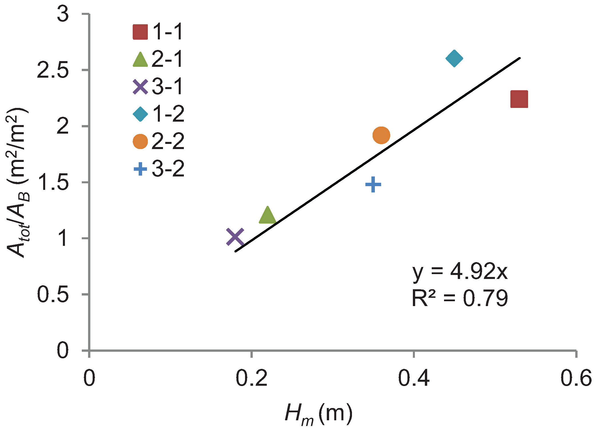
For the investigated test reaches 1–3 (Figure 2) consisting of herbaceous vegetation, a linear regression between the mean heights from 1 cm grid and Atot/AB was derived (Figure 7). The 1 cm grid resolution provided more accurate linear regression (R2 = 0.79) than the 5 cm resolution with R2 = 0.64. The 1 cm grid reflected better the structure of the herbaceous vegetation, as the 5 cm grid did not fully reproduce the variable height distribution in the quadrates and exaggerated the amount of vegetation cover. Using the 1 cm grid size, the standard deviation of the heights varied between 11 and 25 cm. Thus, a larger grid of 10 cm was found inadequate for deriving reliable results. The goodness of fit was larger for the trees in laboratory (Figure 5a) than for the herbaceous vegetation in the field site (Figure 7). The Pearson correlation was statistically significant for both but larger for the woody vegetation than for the herbaceous vegetation (0.904, p < 0.05). This was caused by the varying distances of the scanner to the sampling quadrates in the field site (Figure 2).
Figure 7. Manually determined Atot/AB as a function of TLS-based mean heights per ground area for the six field quadrates (see Table 1 for the vegetation characteristics).
Water 07 00420 g007
The manually measured Atot/AB and dry mass per ground area, (md/AB) values are shown in Table 1 with the TLS point cloud density of the quadrates. The TLS point cloud density (Table 1) corresponds to the number of points in the quadrates. The field TLS dataset demonstrated a common characteristic of TLS measurements, where the point cloud density varies spatially (Table 1). In addition, it may be difficult to position the scanner high enough so that large areas are covered and occlusion is as small as possible. For dense point clouds and sparse vegetation cover (in this case a single tree) where the scanning was subjected to a small occlusion effect, voxels could be applied (Figure 5). Dense herbaceous vegetation considerably occludes the laser beam [30], which prevented the use of voxels. However, in most cases, for herbaceous vegetation using the mean height estimated from the highest elevations in a grid cell may be adequate, as herbaceous vegetation grows fairly uniformly over height in contrast to woody vegetation. The grid resolution of 1 cm is suitable for estimating plant height (e.g., paddy rice [43]), but grid resolutions larger than 1 cm may be sufficient for homogenously growing herbaceous vegetation [44]. The mean height was used for the linear regression; however, in some cases the percentiles (95th, 85th) may be more appropriate [44].
Table 1. Vegetation characteristics from manual samples and the resulting point cloud density in the vegetated quadrates in August 2013.
SampleAtot/AB (m2/m2)md/AB (kg/m2)TLS Density (pts/m2)
1–12.160.237,377
1–22.660.3413,477
2–11.210.147,961
2–21.740.19494,952
3–10.930.14135,618
3–21.040.214,449

3.3. Testing of the Proposed TLS Method for the Characteristic Area Determination

Independent field data were used for the testing of the linear regressions between the total areas and mean heights (herbaceous vegetation) and between the total areas and voxel count (woody vegetation). Three differently vegetated test reaches were explored (Grasses-U and -D, and a test reach growing willows with cut grasses: Willows-M, see [30]). The classification with the Canupo tools [27] selected 50% of the points in the Willows-M as vegetation, while 36% were classified as ground and 14% were unclassified. Some points clearly above the ground surface were classified as ground, but the percentage of the error points was small (≈0.1%). The classification accuracy of the willows was 98.7%. For the herbaceous vegetation, only few points were classified as ground (<1%), as the floodplain was densely covered with vegetation.
The relationship between Atot/AB and Hm (Figure 7) was used for the herbaceous test reaches as Atot/AB = 4.92Hm for each cell. The 1 cm grid resolution was used in the analyses as the vegetation heights varied in the test reaches (see Section 3.1). For the willows, the relationship between Atot and count of the 1 cm voxels derived for the trees was used as Atot/AB = 0.000062Nvox per corresponding grid area (see Figure 5a). The testing with the independent TLS yielded Atot/AB values between 0 and 5.4 for the herbaceous test reaches, and the measured Atot/AB values fell within the ranges of the TLS analyses (Table 2). The Atot/AB ranges and standard deviations in Table 2 are calculated for a 0.12 m grid to be comparable with the manual measurement quadrate size (0.125 × 0.125 m2). The mean Atot/AB for Willows-M was 28% lower from manual measurements in comparison to TLS. For the Grasses-U and -D, the mean Atot/AB value from TLS was one third of the manual measurements. These differences between the TLS and manual sampling of the independent data may be caused by the changes in the herbaceous vegetation during the two years. The differences between the manual sampling and TLS-based Atot/AB for the test reaches emphasize the need for site-specific linear regressions (or species-specific) for the upscaling process (see Section 3.4 for the proposed method).
Table 2. TLS-based areas from the independent field-test data in comparison to the manual sampling.
Test ReachAtot/AB (−)Atot/AB (−) from TLSDescription
ManualMeanRangeSt. Dev.
Grasses-U3.51 11.900.0–5.40.91Sown pasture grasses, upstream reach
Willows-M0.29 20.400.0–5.10.50Small, young willows with cut grasses, maintained
Grasses-D3.41 11.100.0–3.80.51Sown pasture grasses, downstream reach
Note: Data sources: 1 [30,39]; 2 [39].
The spatial distribution of the floodplain vegetation in the test reaches is shown in Figure 8 for the 12-m-long parts of the test reaches. The scale bars show the classification of Atot/AB values in the 30 cm grid. The detected highest elevations were affected by the May DTM accuracy; hence the DTM accuracy also impacted the estimated Atot/AB. The ground level estimated from TLS depends on the vegetation height and density, incidence angle, scan resolution, location, and number of scan stations [30]. For the Grasses-U the DTM error was circa 3 cm (compared to manual cross-sectional survey, see [30]), decreasing the Atot/AB by 10%. For the Grasses-D mean error in DTM of 30 cm window size was circa 5 cm [30], and the ground level inaccuracy reduced the Atot/AB 18%. The application of the linear relationships of the Atot vs. Nvox for 5 cm and 10 cm voxels doubled the Atot/AB in comparison to using the 1 cm voxels (Atot/AB was 0.80 and 0.74 for the 5 and 10 cm voxel sizes, respectively). This can be attributed to the small size (≈1 m) of the willows in the field as the width of the willows including branches was only around 20 cm, and thus the 5 and 10 cm voxel sizes were large in comparison to the tree size.
Figure 8. TLS-based Atot/AB in 30 cm grid in the floodplain area of the test reaches (a) Grasses-U; (b) Willows-M; and (c) Grasses-D.
Water 07 00420 g008

3.4. Summarizing the Process of Characterizing Mixed Floodplain Vegetation from Point Cloud Data
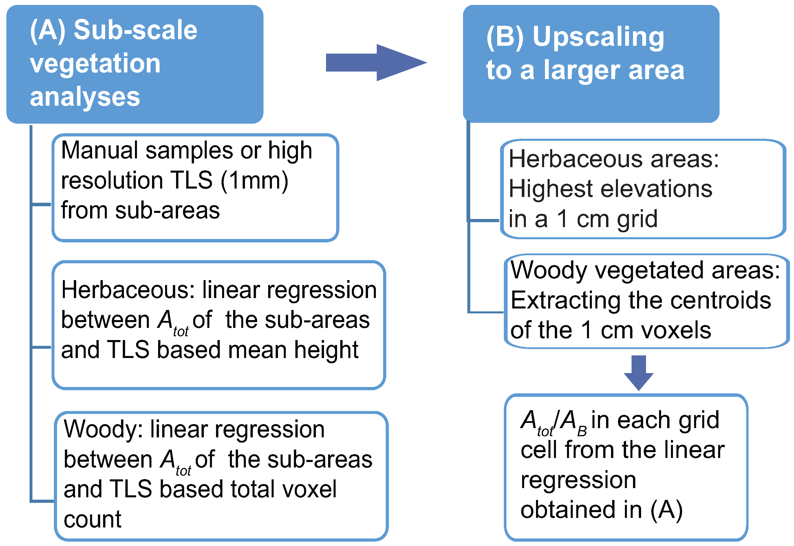
The proposed workflow to estimate the characteristic reference areas of floodplain vegetation is described in Figure 9. The high R2-values of the linear regressions suggested that the relationships between characteristic vegetation area and voxel count or vegetation height can be first derived for each vegetation type from small sub-areas, and upscaled to a reach with similar vegetation cover. The linear regressions of the herbaceous vegetation were significant, but the testing of the linear regressions (Table 2) was only indicative due to differences in the vegetation cover. During the field campaign in 2013 the monitoring of the field site [39] was finished, and the vegetation cover was more variable than the originally established test reaches [39] of the 2011 TLS data [30] used for the testing. Thus, the applicability of the sub-scale linear regressions for the upscaling (Figure 9) remains to be evaluated more thoroughly in future studies.
Figure 9. Floodplain vegetation analyses: Proposed work-flow of processing multi-station TLS point clouds for hydro-environmental modeling applications.
Water 07 00420 g009
The required point cloud resolution and the resulting grid or voxel resolution depended on the vegetation cover. Although the 1 cm voxel size was required for the small thin willows in the field site (Table 2), the 5 cm and 10 cm voxel sizes for the trees in laboratory showed a linear regression with Atot and Nvox, which indicated that larger voxel sizes than 1 cm are adequate in most cases. On the other hand, for the herbaceous vegetation with variable height distribution, a grid resolution of 1 cm was required.
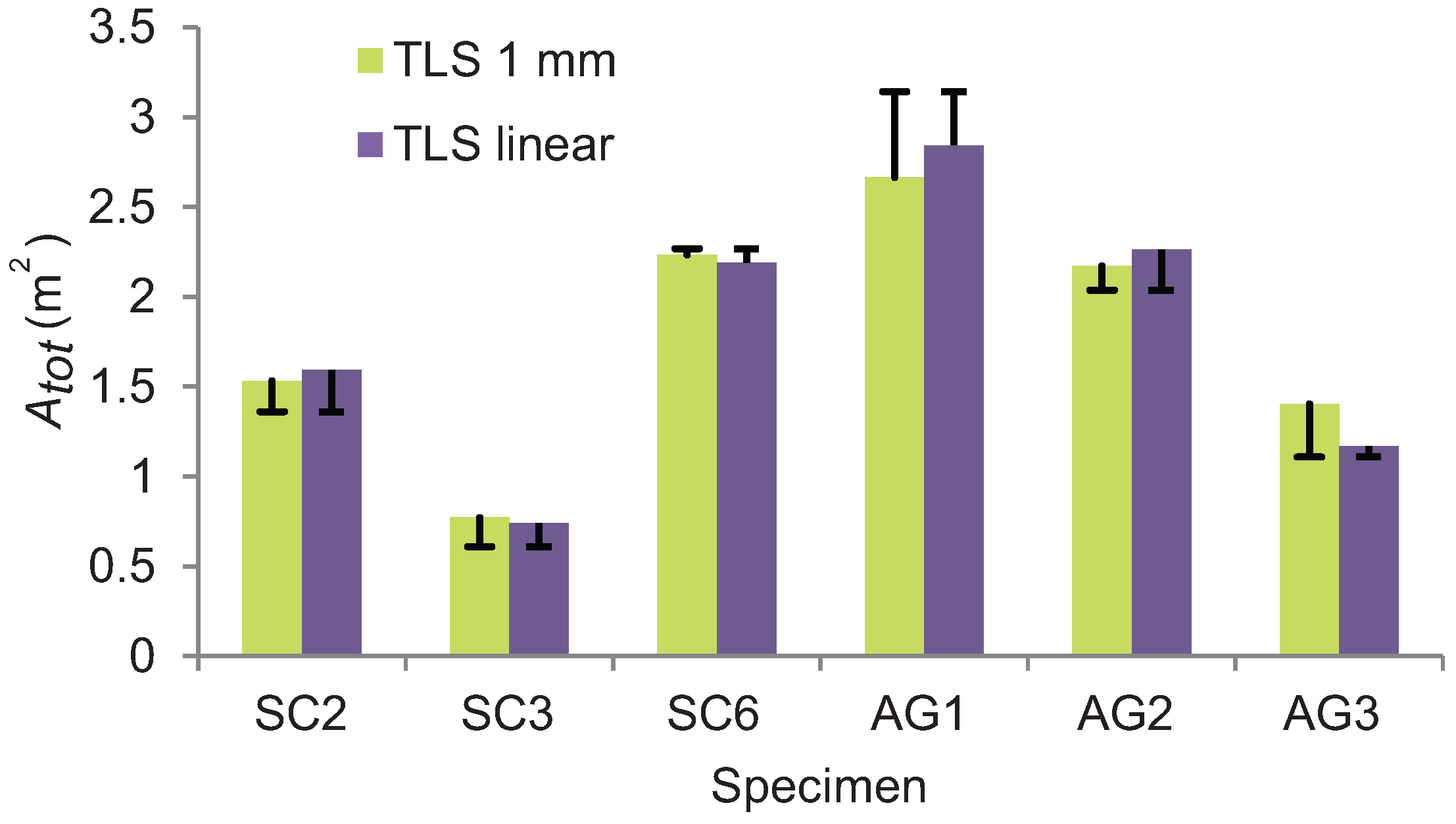
Obtaining the total plant area of a tree manually in the field is invasive and laborious. Thus, the sub-scale total plant area is more viable to estimate from high-resolution scan of the sub-area than by manual sampling. The Atot for sub-areas can be obtained by voxelizing the point cloud to a 1 mm grid [34] and estimating the Atot from the voxel count multiplied with the voxel size (Figure 10). Figure 10 shows the Atot,TLS estimated both with mm resolution TLS and with the linear regression derived in Figure 5. The bars highlight the difference to the manual measurements of Atot as Atot,man–Atot,TLS. The averaged difference of the mm resolution TLS-based Atot in comparison to the manual sampling was 10%. Note that the 1 mm voxelization method used yields twofold values of the actual stem surface area (i.e., the area exposed to the flow, see Section 2.2). To obtain the Atot, the manually measured (one-sided) AS was subtracted from the total one-sided area of the voxels (=Nvox × 1 mm2). To derive the actual AS, the stem area may also be predicted by the basal diameter (Db) [41]. The stem points can also be separated from the foliage by coloring the point cloud by the integrated camera image [21], by intensity values [45] or by selecting the stem manually in TLS software. To separate the stem from the foliage based on intensity values is difficult, as the process is sensitive to the instrument properties such as the wavelength or footprint size, and differences in the leaf spectral properties [35].
Figure 10. The total plant area of the S. caprea and A. glutinosa specimens with 1 mm voxels and back-calculated from the linear regression (Figure 5). The bars denote the difference Atot,man–Atot,TLS.
Water 07 00420 g010
The proposed method for deriving the characteristic reference areas (Figure 9) requires that the vegetation points are classified to different vegetation types either by manual or automatic classification. After the vegetation types are distinguished, the area definitions suitable for each vegetation type are applied (Figure 9).
The geometry-based classification tools designed to distinguish between different types of elements [27] may be feasible for classifying vegetation types. On a larger scale, in a 2 × 2 m grid, MLS point clouds can be classified as bare, field, shrubs, and canopy layer using point cloud statistics (mean height, 95th percentile, [46]). Laser pulse intensity values are used to classify buildings and trees [47], and tree species [48], or the stem (wood material) and foliage of woody vegetation [45]. To locate trees from multi-station TLS, Liang and Hyyppä [49] developed an automatic tree-mapping algorithm. Canopy surfaces and tree positions derived from airborne LiDAR as well as the combination of LiDAR, radar and multispectral data provide useful information for defining areas of different vegetation type [20,31,50].
The developed approach (Figure 9) is not limited to TLS, but can be used for point clouds obtained from different LS and surveying methods depending on the data resolution. Structure-from-motion photogrammetry is a low-cost tool advantageous in generating point clouds in remote riverine environments [51]. Boat-based mobile laser scanning (BoMMS) provide centimeter resolution point data with a boat speed of 1–2 m/s [52], and the BoMMS data set can be improved with point clouds from low-altitude unmanned aerial vehicle (UAV) based photogrammetry [53]. When measurements are conducted from different angles (above, from boat or by combining them with TLS and multiple scan stations), the occlusion effects decrease. The use of multisource data is superior to sole TLS, though combining these data requires accurate relative orientation [32]. For areas of dense vegetation cover, methods that provide point clouds measured from above the vegetation, such as MLS mounted on a backpack [23] or on UAV [52], are expected to provide detailed information about the vegetation structure more efficiently than ground-based TLS.

4. Conclusions

In the context of modeling floodplain flows, a new experimental dataset on characteristic vegetation areas was derived by terrestrial laser scanning (TLS) and evaluated against comprehensive manual measurements. Subsequently, an approach was developed to relate attributes of the TLS data and the vegetation characteristics of small sub-areas to enable upscaling to larger areas of similar vegetation type. Two alternatives were found for determining the relationships between the TLS attributes and total plant area (Atot) of the sub-areas: by millimeter resolution TLS or by collecting manual vegetation samples. Furthermore, the results showed that different methods are needed for woody and herbaceous vegetation. For herbaceous vegetation, the mean heights of the digital surface model appeared sufficient for determining Atot but for woody vegetation voxelization was required. For woody vegetation, a linear regression based on the voxel count was found feasible to estimate both the Atot and its vertical distribution. In performing the sub-area measurements, the use of TLS was considered preferable over laborious and destructive manual sampling, in particular for woody vegetation. It is expected that the use of the regressions acquired for woody vegetation can be extended to other sites with similar vegetation type, but it remains to be investigated how these relationships vary for trees of different sizes and ages. The voxel size of 1 cm was found suitable for describing small thin trees, but for the larger trees 5 and 10 cm voxels appeared adequate. In estimating the mean heights of the herbaceous vegetation, the 1 cm grid size was required as the 5 cm grid was not capable of reproducing the varying height distributions. Due to the variability in the herbaceous vegetation cover, the linear regressions derived between Atot and mean height were considered as site specific. Whether similar linear regressions exist for other types of herbaceous vegetation remains to be investigated. Overall, the LS-based approach presented in this study is expected to be useful in estimating the characteristic areas of mixed vegetation required in hydro-environmental modeling applications. Rapidly developing LS techniques including mobile laser scanning platforms such as backpacks, boats, and unmanned aerial vehicles can be expected to ease the data collection.

Acknowledgments

The study was supported by the Maa- ja vesitekniikan tuki ry, the Academy of Finland (Flow-vegetation-sediment interaction project, grant No. 133113; and the Centre of Excellence in Laser Scanning Research, 272195), Aalto Energy Efficiency Research Programme (Light Energy—Efficient and Safe Traffic Environments project), and the EUE project (2141226).

Author Contributions

All authors were involved in designing the investigations. Johanna Jalonen, Juho-Pekka Virtanen, Matti Vaaja and Matti Kurkela conducted the field TLS campaign; Johanna Jalonen performed the laboratory TLS; Matti Vaaja registered the field point clouds; Johanna Jalonen carried out the data analyses; and Hannu Hyyppä provided insight and guidance on the LS methodology used. Johanna Jalonen wrote the paper with Juha Järvelä and all co-authors took part in the writing process.

Conflicts of Interest

The authors declare no conflict of interest.

References

  1. Aberle, J.; Järvelä, J. Hydrodynamics of vegetated channels. In Rivers—Physical, Fluvial and Environmental Processes, GeoPlanet: Earth and Planetary Sciences; Rowinski, P., Radeck-Pawlik, A., Eds.; Springer: Berlin, Germany, 2015. [Google Scholar]
  2. Gurnell, A. Plants as River System Engineers. Earth Surf. Process. Landf. 2014, 39, 4–25. [Google Scholar]
  3. Aberle, J.; Järvelä, J. Flow Resistance of Emergent Rigid and Flexible Floodplain Vegetation. J. Hydraul. Res. 2013, 51, 33–45. [Google Scholar] [CrossRef]
  4. Anderson, B.G.; Rutherfurd, I.D.; Western, A.W. An Analysis of the Influence of Riparian Vegetation on the Propagation of Flood Waves. Environ. Modell. Softw. 2006, 21, 1290–1296. [Google Scholar] [CrossRef]
  5. Petryk, S.; Bosmajian, G.B. Analysis of Flow through Vegetation. J. Hydraul. Div. 1975, 101, 871–884. [Google Scholar]
  6. Bunting, D.P.; Kurc, S.; Grabau, M. Long-Term Vegetation Dynamics after High-Density Seedling Establishment: Implications for Riparian Restoration and Management. River Res. Appl. 2013, 29, 1119–1130. [Google Scholar] [CrossRef]
  7. Västilä, K.; Järvelä, J. Modeling the Flow Resistance of Woody Vegetation using Physically Based Properties of the Foliage and Stem. Water Resour. Res. 2014, 50, 229–245. [Google Scholar] [CrossRef]
  8. Västilä, K.; Järvelä, J.; Aberle, J. Characteristic Reference Areas for Estimating Flow Resistance of Natural Foliated Vegetation. J. Hydrol. 2013, 492, 49–60. [Google Scholar] [CrossRef]
  9. Jalonen, J.; Järvelä, J.; Aberle, J. Leaf Area Index as Vegetation Density Measure for Hydraulic Analyses. J. Hydraul. Eng. 2013, 139, 461–469. [Google Scholar] [CrossRef]
  10. Jalonen, J.; Järvelä, J.; Aberle, J. Vegetated Flows: Drag Force and Velocity Profiles for Foliated Plant Stands. In River Flow 2012, Proceedings of the International Conference on Fluvial Hydraulics, San José, Costa Rica, 5–7 September 2012; pp. 233–239.
  11. Jalonen, J.; Järvelä, J. Estimation of Drag Forces Caused by Natural Woody Vegetation of Different Scales. J. Hydrodyn. 2014, 26, 608–623. [Google Scholar] [CrossRef]
  12. Whittaker, P.; Wilson, C.; Aberle, J.; Rauch, H.P.; Xavier, P. A Drag Force Model to Incorporate the Reconfiguration of Full-Scale Riparian Trees under Hydrodynamic Loading. J. Hydraul. Res. 2013, 51, 569–580. [Google Scholar] [CrossRef]
  13. Green, J.C. Effect of Macrophyte Spatial Variability on Channel Resistance. Adv. Water Resour. 2006, 29, 426–438. [Google Scholar] [CrossRef]
  14. Nikora, V. Hydrodynamics of Aquatic Ecosystems: An Interface between Ecology, Biomechanics and Environmental Fluid Mechanics. River Res. Appl. 2010, 26, 367–384. [Google Scholar] [CrossRef]
  15. Luhar, M.; Nepf, H.M. From the Blade Scale to the Reach Scale: A Characterization of Aquatic Vegetative Drag. Adv. Water Resour. 2013, 51, 305–316. [Google Scholar] [CrossRef]
  16. Green, J.C. Comparison of Blockage Factors in Modelling the Resistance of Channels Containing Submerged Macrophytes. River Res. Appl. 2005, 21, 671–686. [Google Scholar] [CrossRef]
  17. Järvelä, J. Determination of Flow Resistance Caused by Non-submerged Woody Vegetation. Int. J. River Basin Manag. 2004, 2, 61–70. [Google Scholar] [CrossRef]
  18. Katul, G.G.; Poggi, D.; Ridolfi, L. A Flow Resistance Model for Assessing the Impact of Vegetation on Flood Routing Mechanics. Water Resour. Res. 2011, 47. [Google Scholar] [CrossRef]
  19. Nepf, H.; Ghisalberti, M. Flow and Transport in Channels with Submerged Vegetation. Acta Geophys. 2008, 56, 753–777. [Google Scholar] [CrossRef]
  20. Forzieri, G.; Castelli, F.; Preti, F. Advances in Remote Sensing of Hydraulic Roughness. Int. J. Remote Sens. 2012, 33, 630–654. [Google Scholar] [CrossRef]
  21. Straatsma, M.W.; Baptist, M.J. Floodplain Roughness Parameterization using Airborne Laser Scanning and Spectral Remote Sensing. Remote Sens. Environ. 2008, 112, 1062–1080. [Google Scholar] [CrossRef]
  22. Straatsma, M.W.; Warmink, J.J.; Middelkoop, H. Two Novel Methods for Field Measurements of Hydrodynamic Density of Floodplain Vegetation using Terrestrial Laser Scanning and Digital Parallel Photography. Int. J. Remote Sens. 2008, 29, 1595–1617. [Google Scholar] [CrossRef]
  23. Kukko, A.; Kaartinen, H.; Hyyppä, J.; Chen, Y. Multiplatform Mobile Laser Scanning: Usability and Performance. Sensors 2012, 12, 11712–11733. [Google Scholar] [CrossRef]
  24. Hodge, R.; Brasington, J.; Richards, K. In situ Characterization of Grain-Scale Fluvial Morphology using Terrestrial Laser Scanning. Earth Surf. Process. Landf. 2009, 34, 954–968. [Google Scholar]
  25. Brasington, J.; Vericat, D.; Rychkov, I. Modeling River Bed Morphology, Roughness, and Surface Sedimentology using High Resolution Terrestrial Laser Scanning. Water Resour. Res. 2012, 48. [Google Scholar] [CrossRef]
  26. Resop, J.; Hession, W. Terrestrial Laser Scanning for Monitoring Streambank Retreat: Comparison with Traditional Surveying Techniques. J. Hydraul. Eng. 2010, 136, 794–798. [Google Scholar] [CrossRef]
  27. Brodu, N.; Lague, D. 3D Terrestrial Lidar Data Classification of Complex Natural Scenes using a Multi-Scale Dimensionality Criterion: Applications in Geomorphology. ISPRS J Photogramm. Remote Sens. 2012, 68, 121–134. [Google Scholar] [CrossRef] [Green Version]
  28. Resop, J.P.; Kozarek, J.L.; Hession, W.C. Terrestrial Laser Scanning for Delineating in-Stream Boulders and Quantifying Habitat Complexity Measures. Photogramm. Eng. Remote Sens. 2012, 78, 363–371. [Google Scholar] [CrossRef]
  29. Smith, M.W.; Vericat, D. Evaluating Shallow-Water Bathymetry from Through-Water Terrestrial Laser Scanning Under a Range of Hydraulic and Physical Water Quality Conditions. River Res. Appl. 2013, 30, 905–924. [Google Scholar] [CrossRef]
  30. Jalonen, J.; Järvelä, J.; Koivusalo, H.; Hyyppä, H. Deriving Floodplain Topography and Vegetation Characteristics for Hydraulic Engineering Applications by Means of Terrestrial Laser Scanning. J. Hydraul. Eng. 2014, 140. [Google Scholar] [CrossRef]
  31. Forzieri, G.; Guarnieri, L.; Vivoni, E.R.; Castelli, F.; Preti, F. Spectral-ALS Data Fusion for Different Roughness Parameterizations of Forested Floodplains. River Res. Appl. 2011, 27, 826–840. [Google Scholar]
  32. Rönnholm, P.; Hyyppä, H.; Hyyppä, J.; Haggrén, H. Orientation of Airborne Laser Scanning Point Clouds with Multi-View, Multi-Scale Image Blocks. Sensors 2009, 9, 6008–6027. [Google Scholar] [CrossRef] [PubMed]
  33. Manners, R.; Schmidt, J.; Wheaton, J.M. Multiscalar Model for the Determination of Spatially Explicit Riparian Vegetation Roughness. Earth Surf. Process. Landf. 2013, 118, 65–83. [Google Scholar]
  34. Hosoi, F.; Omasa, K. Voxel-Based 3-D Modeling of Individual Trees for Estimating Leaf Area Density using High-Resolution Portable Scanning Lidar. IEEE Trans. Geosci. Remote Sens. 2006, 44, 3610–3618. [Google Scholar] [CrossRef]
  35. Béland, M.; Widlowski, J.; Fournier, R.A. A Model for Deriving Voxel-Level Tree Leaf Area Density Estimates from Ground-Based LiDAR. Environ. Model. Softw. 2014, 51, 184–189. [Google Scholar] [CrossRef]
  36. Radtke, P.J.; Bolstad, P.V. Laser Point-Quadrat Sampling for Estimating Foliage-Height Profiles in Broad-Leaved Forests. Can. J. For. Res. 2001, 31, 410–418. [Google Scholar] [CrossRef]
  37. Antonarakis, A.S.; Richards, K.S.; Brasington, J.; Muller, E. Determining Leaf Area Index and Leafy Tree Roughness using Terrestrial Laser Scanning. Water Resour. Res. 2010, 46. [Google Scholar] [CrossRef]
  38. Guarnieri, A.; Vettore, A.; Pirotti, F.; Menenti, M.; Marani, M. Retrieval of Small-Relief Marsh Morphology from Terrestrial Laser Scanner, Optimal Spatial Filtering, and Laser Return Intensity. Geomorphology 2009, 113, 12–20. [Google Scholar] [CrossRef]
  39. Västilä, K.; Järvelä, J. Cohesive Sediment Dynamics in a Vegetated Two-Stage Drainage Channel: The First Year after Floodplain Excavation. In Proceedings of the 7th International Symposium on River, Coastal and Estuarine Morphodynamics, RCEM, Tsinghua University, Beijing, China, 6–8 September 2011; pp. 1481–1489.
  40. Rusu, R.B.; Marton, Z.C.; Blodow, N.; Dolha, M.; Beetz, M. Towards 3D Point Cloud Based Object Maps for Household Environments. Semant. Knowl. Robot. 2008, 56, 927–941. [Google Scholar]
  41. Weissteiner, C.; Rauch, H.P.; Jalonen, J.; Järvelä, J. Spatial-Structural Analysis of Woody Riparian Vegetation for Hydraulic Considerations. In Proceedings of the 35th IAHR World Congress, Chengdu, China, 8–13 September 2013.
  42. Bréda, N.J.J. Ground-Based Measurements of Leaf Area Index: A Review of Methods, Instruments and Current Controversies. J. Exp. Bot. 2003, 54, 2403–2417. [Google Scholar] [CrossRef] [PubMed]
  43. Tilly, N.; Hoffmeister, D.; Cao, Q.; Huang, S.; Lenz-Wiedemann, V.; Miao, Y.; Bareth, G. Multitemporal Crop Surface Models: Accurate Plant Height Measurement and Biomass Estimation with Terrestrial Laser Scanning in Paddy Rice. J. Appl. Remote Sens. 2014, 8. [Google Scholar] [CrossRef]
  44. Radtke, P.J.; Boland, H.T.; Scaglia, G. An Evaluation of Overhead Laser Scanning to Estimate Herbage Removals in Pasture Quadrats. Agric. For. Meteorol. 2010, 150, 1523–1528. [Google Scholar] [CrossRef]
  45. Béland, M.; Widlowski, J.; Fournier, R.A.; Côté, J.; Verstraete, M.M. Estimating Leaf Area Distribution in Savanna Trees from Terrestrial LiDAR Measurements. Agric. For. Meteorol. 2011, 151, 1252–1266. [Google Scholar] [CrossRef]
  46. Saarinen, N.; Vastaranta, M.; Vaaja, M.; Lotsari, E.; Jaakkola, A.; Kukko, A.; Kaartinen, H.; Holopainen, M.; Hyyppä, H.; Alho, P. Area-Based Approach for Mapping and Monitoring Riverine Vegetation using Mobile Laser Scanning. Remote Sens. 2013, 5, 5285–5303. [Google Scholar] [CrossRef]
  47. Kaasalainen, S.; Lindroos, T.; Hyyppä, J. Toward Hyperspectral Lidar: Measurement of Spectral Backscatter Intensity with a Supercontinuum Laser Source. IEEE Geosci. Remote Sens. Lett. 2007, 4, 211–215. [Google Scholar] [CrossRef]
  48. Holmgren, J.; Persson, Å. Identifying Species of Individual Trees using Airborne Laser Scanner. Remote Sens. Environ. 2004, 90, 415–423. [Google Scholar] [CrossRef]
  49. Liang, X.; Hyyppä, J. Automatic Stem Mapping by Merging several Terrestrial Laser Scans at the Feature and Decision Levels. Sensors 2013, 13, 1614–1634. [Google Scholar] [CrossRef] [PubMed]
  50. Forzieri, G.; Guarnieri, L.; Vivoni, E.R.; Castelli, F.; Preti, F. Multiple Attribute Decision Making for Individual Tree Detection using High-Resolution Laser Scanning. For. Ecol. Manag. 2009, 258, 2501–2510. [Google Scholar] [CrossRef]
  51. Westoby, M.J.; Brasington, J.; Glasser, N.F.; Hambrey, M.J.; Reynolds, J.M. “Structure-from-Motion” Photogrammetry: A Low-Cost, Effective Tool for Geoscience Applications. Geomorphology 2012, 179, 300–314. [Google Scholar] [CrossRef] [Green Version]
  52. Vaaja, M.; Kukko, A.; Kaartinen, H.; Kurkela, M.; Kasvi, E.; Flener, C.; Hyyppä, H.; Hyyppä, J.; Järvelä, J.; Alho, P. Data Processing and Quality Evaluation of a Boat-Based Mobile Laser Scanning System. Sensors 2013, 13, 12497–12515. [Google Scholar] [CrossRef] [PubMed]
  53. Flener, C.; Vaaja, M.; Jaakkola, A.; Krooks, A.; Kaartinen, H.; Kukko, A.; Kasvi, E.; Hyyppä, H.; Hyyppä, J.; Alho, P. Seamless Mapping of River Channels at High Resolution using Mobile LiDAR and UAV-Photography. Remote Sens. 2013, 5, 6382–6407. [Google Scholar] [CrossRef]