Mean Normalized Force Computation for Different Types of Obstacles due to Dam Break Using Statistical Techniques

Abstract

The dam-break induced loads and their effects on buildings are of vital importance for assessing the vulnerability of buildings in flood-prone areas. A comprehensive methodology, for risk assessment of buildings subject to flooding, is nevertheless still missing. This research aims to take a step forward by following previous research. To this aim, (1) five statistical procedures including: simple correlation analysis, multiple linear regression model, stepwise multiple linear regression model, principal component analysis and cluster analysis are used to study relationship between mean normalized force on structure and other related variables; (2) a new and efficient variable that can take into account both the shape of the structure and flow conditions is proposed; (3) a new and practical formula for predicting the mean normalized force is suggested for different types of obstacles, which is missing in the previous research.

1. Introduction

Dam break wave corresponds to an uncontrolled release of a mass of fluid in a channel due to the structure failure. From the hydrodynamic point of view, dam break flow is characterized by shockwaves, subcritical, supercritical and trans-critical flows [1]. Surge waves induced by dam break may cause serious floods with numerous casualties and damages. The surge front is characterized by sudden flow discontinuities and variation in depth and velocity. Although it is a rather explored problem, dam break wave propagation down the rough surface remains impossible to solve because of all influencing parameters.

Dam break wave propagation is one of the most studied examples of unsteady open channel flow. Even though, there are still arguments about the driving constitutes of unsteady turbulent flow influence, such as spatial and temporal variation, bottom slope, friction characteristics, and speed of failure. Major dam breaks in the past century such as failures of the St Francis Dam (1928), Malpasset Dam (1959) and overtopping of the Vajont Dam (1963) attracted recent attention to the subject [2].

Basics of dam break wave profile are explained with some basic assumptions. The first one who attempted to describe dam break wave profile applying method of characteristics on solution of differential form of Saint-Venant equations was [3]. Ever since, many analytical and numerical methods have been developed in order to simulate dam break flows. As the dam break wave propagates downstream with rapidly increasing speed, it generates strong impact forces on structures and obstacles. For the flood risk assessment and safety concepts, it is important to estimate the impact forces properly.

2. Literature Review

Forces on structures, associated with dam break, are generated by hydrostatic and hydrodynamic loading on structures.

Hydrostatic forces, F_hs, are generated by pressure on the vertical side of structure and buoyancy on the horizontal side. Some of the existing codes propose calculation of hydrostatic force per unit width with velocity head component, while Federal Emergency Management Agency suggests formulation of force without velocity head, assuming it to be insignificant component of the hydrostatic force [Equation (1)] [4].

(1)

where, g is acceleration due to gravity, h_us and h_ds are the water depths upstream and downstream of the structure, respectively, and ρ is density of the fluid. The effect of buoyant force, F_b, cannot be neglected as it affects the resistance of structure against sliding and overturning. It can be calculated as follows [Equation (2)]:

(2)

where V is volume of water displaced by submerged structure.

Hydrodynamic forces, F_hd, are induced by loading, which consists of drag/velocity dominated (quasi-static) loading and inertia/acceleration dominated (impulsive) loading. Hydrodynamic forces are dependent on kinematics of the flow as well as the geometry and dynamic characteristics of the structure. Although the general expression of this force [Equation (3)] is recommended by existing codes, there are still ambiguities in defining it.

(3)

F_hd is the total drag force acting in the direction of flow, b·h is area of the structural element normal to the flow direction, C_d is the drag coefficient, which is highly dependent on Reynolds number and shape of the obstacles, and u is flow velocity component orthogonal to the structure. This expression is widely used with variation in drag coefficient values, depending on the geometry of the affected structure. Federal Emergency Management Agency recommends drag coefficient 2.0 for rectangular piles and 1.0 and 1.2 for circular piles [4]. Although recommended, Equation (3) does not involve inertia as an important factor in total hydrodynamic force. The more complete relationship is given as follows [5]:

(4)

where C_1,1 and C_1,2 are inertia coefficients related to variation of flow velocity and water depth, as these two parameters have significant influence to damage of the structure affected.

First experimental and analytical researches which tried to quantify forces due to hydraulic bore reach dates back to Cumberbatch [6], who tried to estimate tsunami impact on the wall and gave solution of a two dimensional fluid impact on a vertical wall. Cross [7] studied surge impact on vertical walls and improved formula of Cumberbatch [6] by adding gravity forces [Equation (5)]:

(5)

where C_F is the force coefficient which is function of the impacted wedge angle.

Ramsden [8] observed the interaction of tsunamis with a vertical wall and found that the maximum measured force due to bores, surges and solitary waves propagating on dry bed is exceeded by the force computed from the maximum measured run-up, assuming hydrostatic conditions. Due to the vertical accelerations, model of Cross [7] under predicts the measured forces due to bore on dry bed by 30%–50%. In addition, empirical formulae for the maximum force due to bore impact and resulting moment exerted on a vertical wall, is developed [Equations (6) and (7)]:

(6)

(7)

where F is force on the wall, F_l force on the wall due to a run-up equal to twice the wave height, assuming hydrostatic pressure; H is the wave height at the wall, h_o is still water depth, M is moment on the wall corresponding to the force F and M_l is the moment corresponding to the force F_l.

Surge forces, F_s, are hydrodynamic forces generated by the impingement of the advancing water front of the bore against the structure. There are still uncertainties about calculation of surge force due to bore. The most applicable formulation is recommended by City and County of Honolulu BuildingCode (CCH) [9], based on Dames and Moore [10], in Equation (8):

(8)

Impulsive forces, F_imp, are hydrodynamic forces caused by initial impact of the leading edge of the bore [11]. According to Ramsden [8], the wave force over dry bed due to impulsive force does not exceed the expected drag force. However, a significant increase was observed on wet bed tests. As flood wave come in set of subsequent waves, the initial wave might not cause any impulsive forces, but the waves traveling over flooded terrain subsequently may cause impulsive forces on structures. Moreover, there are some other studies on dam-break phenomena in the literature. Researches on fluid–structure interactions after a dam break were initiated [1,12]. Laboratory tests concerning dam break flows were carried out in straight and curved channels [13]. Initial stages of the dam break flow were well detected by recording the flow using CCD cameras [14]. Several numerical studies based on shallow water equations have been compared with experimental data of the dam break flow over channel with bottom obstacle [15]. Oertel et al. [16] studied on 2D dam-break waves comparing physical and numerical data as well as analytical approaches. For various placed obstacles in the propagation area, drag forces are also analyzed and compared. Soares-Frazão and Zech [17] searched the dam break phenomena break in channels with 90-degree bend. Chanson [18] applied the method of characteristics to the dam break wave problem.

Arnason [19] reached similar conclusions in his experimental work. Design standards [4], in which results of Arnason [19] are included, recommend calculation of hydrodynamic force, acting on isolated building, as in Equation (3). They suggest applying C_d = 3 in the equation to account for the impulsive component of the force, which implies formulation of impulsive force as:

(9)

In this study, the most recent test results by Arnason et al. [19,20] are followed to develop an efficient and practical formula for predicting mean normalized forces exerting on different types of obstacles, in terms of engineering design perspective. For this purpose, (1) five statistical procedures are performed to investigate both the most parsimonious and most appropriate model that cannot violate the restrictive assumptions; (2) new variable that can take into account the shape of the obstacles exposed to dam break wave is suggested; (3) a new and practical formula for predicting the mean normalized force is suggested for different types of obstacles, which is missing in the previous research.

3. Experiments

In this study, experimental results of Arnason et al. [19,20] are used for predicting mean normalized forces on obstacles due to dam-break. The experiments are performed in a wave channel, which is 16.6 m long, 0.6 m wide and 0.45 m deep, with glass sidewalls. The bores are generated by lifting a 6.4 mm thick stainless steel gate, which initially separated a thin layer of water from the impoundment behind the gate. The gate was lifted in 0.2 s or less by a 64 mm diameter pneumatic cylinder driven by 0.5 MPa air pressure. A similar generation scheme as adopted was previously used by Ramsden [8] and Yeh et al. [21], which is capable of generating precise bores. The obstacles, which mimic structures in the tests, are three circular columns of varying diameters (Ds) as 140 mm, 60.6 mm and 29 mm, which will be referred to as large, medium and small, and two square columns (SCs) of 120 mm × 120 mm size in two different configurations, which will be referred to as square and diamond. The test matrix that is used in this study is tabulated in Table 1.

The normalized resistance coefficient is given as , with F_x being force in the x-direction, ρ being density of the water during runs as 998 kg/m³, h being the bore height, b being width of the object perpendicular to the flow, and finally u being the flow velocity. In this study the mean normalized force, is timely averaged within interval t₁–t₂ as [Equation (10)]:

(10)

Table 1. Test matrix of [19].

h1	Large	Medium	Small	Rectangular	Diamond
	D = 140mm	D = 60.6mm	D = 29mm	SC = 120 mm × 120 mm	SC = 120 mm × 120 mm
100 mm	+	+	+	+	+
125 mm	+	x	x	+	+
150 mm	+	+	x	+	+
175 mm	x	x	x	+	+
200 mm	+	+	+	+	+
225 mm	+	x	x	+	+
250 mm	+	+	+	+	+
275 mm	+	x	x	+	+
300 mm	+	+	+	+	+

Notes: h₁: height of impoundment behind the gate [20,21]; +: test completed; x: test not completed; →: bore direction.

Table 1. Test matrix of [19].

h1	Large	Medium	Small	Rectangular	Diamond
	D = 140mm	D = 60.6mm	D = 29mm	SC = 120 mm × 120 mm	SC = 120 mm × 120 mm
100 mm	+	+	+	+	+
125 mm	+	x	x	+	+
150 mm	+	+	x	+	+
175 mm	x	x	x	+	+
200 mm	+	+	+	+	+
225 mm	+	x	x	+	+
250 mm	+	+	+	+	+
275 mm	+	x	x	+	+
300 mm	+	+	+	+	+

Notes: h₁: height of impoundment behind the gate [20,21]; +: test completed; x: test not completed; →: bore direction.

4. The Statistical Analysis

The study is motivated by the problem of generating new efficient formula for better understanding of dam-break induced forces on structures of different cross sections, which is missing in Arnason [19].

In regression analysis, as the parameters are entered into the model, whether or not they have relationship with the output, it is highly possible that one can get higher R² but more important parameter is the “the adjusted R²”, indicating degree to which the related variable belongs. Therefore, statistical tests are performed in each regression model to better understand the relationship between variables. Second important factor in regression analysis is to construct parsimonious models in terms of engineering perspective, even if the predicting capability could drop in statistical error criteria. In this research, both of the two aspects are considered.

Some statistical analyzing techniques are applied to define the most influential parameters between and other nondimensional parameters as R_eh, R_eb, F_r, h/b, in which R_eh = is the flow Reynolds number, R_eb = is the object Reynolds number, with being kinematic viscosity and u the flow velocity. F_r = is the Froude number, in which h is the bore height.

4.1. Basic Statistics and Simple Correlation Analysis

Table 2 shows the minimum and maximum values, mean and standard deviations for all variables of in order to summarize the characteristics of a data set.

Table 2. Basic statistics.

		Reb (×105)	Reh (×104)	h/b	Fr
Min.	0.89	0.17	2.28	0.29	0.86
Max.	2.26	2.19	12.77	3.42	1.31
Mean	1.74	1.14	7.32	0.87	1.13
St. Dev.	0.42	0.55	3.56	0.73	0.15

Table 2. Basic statistics.

		Reb (×105)	Reh (×104)	h/b	Fr
Min.	0.89	0.17	2.28	0.29	0.86
Max.	2.26	2.19	12.77	3.42	1.31
Mean	1.74	1.14	7.32	0.87	1.13
St. Dev.	0.42	0.55	3.56	0.73	0.15

Correlation coefficients between and its components are calculated in Table 3. The correlation matrix is useful for checking the pattern of relationship between pairs. It must be noted that correlation coefficient does neither identify causality nor measure nonlinear association, but only linear association. Therefore, correlation analysis is performed to select statistically significant variables that have strong relationship with , considering only the linear relationship. In correlation analysis, the values close to “1” mean there is a strong relationship, whereas “0” indicates that the two variables are independent of each other. It is demonstrated in Table 3 that is highly correlated with h/b, R_eh, F_r, whereas lowly with R_eb. The most linearly correlated parameter to is h/b. It should be taken into account, unfortunately, that variables except h/b, are correlated with each other in a medium level, which may cause collinearity problem in regression analysis.

Table 3. Correlation coefficients.

	Cr	Reb	h/b	Reh	Fr
Cr	1.000	0.239	−0.767	−0.500	−0.472
Reb	0.239	1.000	−0.548	0.480	0.511
h/b	−0.767	−0.548	1.000	0.376	0.339
Reh	−0.500	0.480	0.376	1.000	0.960
Fr	−0.472	0.511	0.339	0.960	1.000

Table 3. Correlation coefficients.

	Cr	Reb	h/b	Reh	Fr
Cr	1.000	0.239	−0.767	−0.500	−0.472
Reb	0.239	1.000	−0.548	0.480	0.511
h/b	−0.767	−0.548	1.000	0.376	0.339
Reh	−0.500	0.480	0.376	1.000	0.960
Fr	−0.472	0.511	0.339	0.960	1.000

4.2. Multiple Linear Regression Model

Linear regression is used to model the value of a dependent scale variable, based on its linear relationship to one or more predictors, which assumes that there is a linear relationship between dependent variable Y_i and its predictors. This relationship is described in the following formula as [Equation (11)]:

(11)

where b indicates regression coefficients, i is case number, p is the predictor indices and e is the error of observed value for i_th case. In our model is the dependent variable whereas F_r, R_eh, R_eb and h/b variables are independent. The R² of linear regression model is 0.642 while adjusted R² is 0.595. Usually, the more predictors included, the higher R² is obtained. Hence, adjusted R² is suggested for model complexity to provide a more fair comparison of model performance. The adjusted R² is calculated as [Equation (12)]:

(12)

where R² is the square of multiple correlation coefficient, p is number of input fields, C is sum of case weights and p* is number of coefficients in the model. If the intercept is included p* = p + 1, otherwise p* = p. Table 4 represents the coefficient statistics, correlations and collinearity statistics. To interpret contribution of the predictors to the regression, it is not sufficient to take into account only the regression coefficients. To determine the relative importance of the significant predictors, the most known evaluation parameter is the standardized coefficient. Even though R_eh has a lower coefficient (unstandardized) than F_r, it contributes more to the model because it has larger absolute standardized coefficient when compared to F_r. The most contributing variable of the model is h/b, with the highest standardized and unstandardized coefficients, 0.739 and 0.428, respectively. The rest are found to be insignificant contributors by t statistics when four variables are constrained to enter the model.

Table 4. Linear regression statistics.

Model	Unstandardized Coefficients		Standardized Coefficients	t	Significance	Correlations			Collinearity Statistics		Collinearity Diagnostics
	B	Std. Error	Beta			Zero-order	Partial	Part	Tolerance	VIF	Eigen value	Condition Index
Constant	2.48	0.93	–	2.67	0.01	–	–	–	–	–	4.41	1.00
Reb	−0.06	0.23	−0.07	−0.25	0.80	0.24	−0.05	−0.03	0.14	7.24	0.47	3.07
Reh	−0.02	0.05	−0.13	−0.32	0.75	−0.50	−0.06	−0.03	0.07	14.62	0.11	6.40
h/b	−0.43	0.16	−0.74	−2.70	0.01	−0.77	−0.44	−0.30	0.16	6.26	0.01	18.77
Fr	−0.16	1.14	−0.06	−0.14	0.89	−0.47	−0.03	−0.02	0.07	14.14	0.00	75.14

Table 4. Linear regression statistics.

Model	Unstandardized Coefficients		Standardized Coefficients	t	Significance	Correlations			Collinearity Statistics		Collinearity Diagnostics
	B	Std. Error	Beta			Zero-order	Partial	Part	Tolerance	VIF	Eigen value	Condition Index
Constant	2.48	0.93	–	2.67	0.01	–	–	–	–	–	4.41	1.00
Reb	−0.06	0.23	−0.07	−0.25	0.80	0.24	−0.05	−0.03	0.14	7.24	0.47	3.07
Reh	−0.02	0.05	−0.13	−0.32	0.75	−0.50	−0.06	−0.03	0.07	14.62	0.11	6.40
h/b	−0.43	0.16	−0.74	−2.70	0.01	−0.77	−0.44	−0.30	0.16	6.26	0.01	18.77
Fr	−0.16	1.14	−0.06	−0.14	0.89	−0.47	−0.03	−0.02	0.07	14.14	0.00	75.14

Partial Correlation and part correlation statistics are presented in Table 4. Partial correlation is correlation between a dependent and an independent variable when linear effects of other independent variables in the model have been removed from both dependent and independent variables. If the linear effect of other variables is removed only from the examined independent variable, but not from dependent variable, this time correlation is named as part correlation. Therefore, part correlation can also be viewed as decrease in R square that results from removing a predictor from the model and sometimes called the semi partial correlation. The values of the partial and part correlations for all the parameters except h/b drop sharply from the zero-order correlation, implying that some variances in are explained by R_eb, F_r and R_eb together. The second part of Table 4 is reserved to most known collinearity statistics and diagnostics. The tolerance is the percentage of the variance in a given predictor that cannot be explained by the other predictors. Thus, the small tolerances show that a high proportion of the variance in a given predictor can be explained by the other predictors. When the tolerances are close by “0” as an indication of high multicollinearity then standard error of the regression coefficients will be inflated. By definition, variance inflation factors (VIF) are inversely related to the tolerances. A VIF that is greater than 2 is usually considered problematic. The smallest VIF in the Table 4 is 6.264 for h/b. Other collinearity diagnostics, condition indexes, confirm that there are serious problems with multicollinearity. The condition indices are computed as the square roots of the ratios of the largest eigenvalue to each successive eigenvalue. The values of condition indices that are greater than 15 indicate a possible problem with collinearity while greater than 30 is a serious problem. One of the condition indices is larger than 30, suggesting a very serious problem with collinearity. Although a serious multicollinearity problem exists, the linear model indicates that the most predictive variable is h/b.

4.3. Stepwise Multiple Linear Regression Model

This procedure was used to determine the variable accounting for the majority of total yielded variability. In stepwise regression process, at each step, an independent variable that has the smallest probability of F is entered in regression. The variables that are already in the regression equation are removed if their F distribution probability becomes sufficiently larger than determined criteria.

In this study, the criteria was determined as; probability of F ≤ 0.050 to enter, whereas F >0.1 to remove. From the perspective of collinearity, all variables must pass the tolerance criterion defined above to enter the regression equation, regardless of the entry method criteria. The tolerance level was determined as so small (0.0001), to gain all the variables in regression except perfectly correlated variables in which the tolerance is 0.000. In addition, a variable was not entered into regression if it would cause tolerance violation of other variables of regression. The dependent and four independent variables were used to construct the stepwise model. The regression statistics of final step are gathered in Table 5. Tolerance, VIF and condition index values show that the regression model is not ill from collinearity. Stepwise model is consisted of two steps and only two variables, h/b and R_eh, are included in the final regression step, as these variables are found significant in regression. R_eb and F_r are found to be insignificant to predict , so these variables are not included in regression. The R² change is only 0.052 when R_eh is entered in model in the second step. As seen from R² change, the contribution of R_eh is very limited when compared to h/b to regress the . The ratio of the absolute values of standardized coefficients show that h/b is about three times more important than R_eh (have more contribution rate in the prediction) to regress .

Table 5. Stepwise regression statistics of final (second) step.

Model	Unstandardized Coefficients		Standardized Coefficients	t	Significance	Correlations			Collinearity Statistics		Collinearity Diagnostics
	B	Std. Error	Beta			Zero-order	Partial	Part	Tolerance	VIF	Eigen value	Cond. Index
Constant	2.30	0.10	–	22.06	0.00	–	–	–	–		2.65	1.00
h/b	−0.39	0.07	−0.67	−5.90	0.00	−0.77	−0.72	−0.63	0.86	1.16	0.25	3.23
Reh	−0.03	0.01	−0.25	−2.15	0.04	−0.50	−0.36	−0.23	0.86	1.16	0.10	5.23

Table 5. Stepwise regression statistics of final (second) step.

Model	Unstandardized Coefficients		Standardized Coefficients	t	Significance	Correlations			Collinearity Statistics		Collinearity Diagnostics
	B	Std. Error	Beta			Zero-order	Partial	Part	Tolerance	VIF	Eigen value	Cond. Index
Constant	2.30	0.10	–	22.06	0.00	–	–	–	–		2.65	1.00
h/b	−0.39	0.07	−0.67	−5.90	0.00	−0.77	−0.72	−0.63	0.86	1.16	0.25	3.23
Reh	−0.03	0.01	−0.25	−2.15	0.04	−0.50	−0.36	−0.23	0.86	1.16	0.10	5.23

4.4. Principal Component Analysis

The principal component analysis is performed by including all four inputs as R_eb, h/b, R_eh, F_r.

The variables in the system have to be intercorrelated, but they should not demonstrate extreme multicollinearity and singularity as this might cause difficulties in determining the unique contribution of the variables to a factor. The variables F_r and R_eh show high correlation because both are derived from the velocity, u, and bore height, h. Therefore, the variable F_r is excluded from the Principal Component Analysis to prevent singularity, which is the extreme form of multicollinearity.

The Kaiser–Meyer–Olkin (KMO) test is performed, which is a measure of sampling adequacy whether partial correlations among variables are small or not. The sample is regarded as adequate if the value of KMO is greater than “0.5”. In the analysis, KMO is calculated as 0.526, which is greater than 0.5. Bartlett’s test of sphericity is applied to check if correlation matrix is an identity matrix, which could imply that variables are unrelated and therefore unsuitable for structure detection. Small values (less than 0.05) of the significance level indicate that factor analysis is valid. In the analysis, Bartlett’s test of sphericity is found to be 0, which is less than 0.05.

The next step is to determine number of factors to be retained. Several rules of thumb have been suggested in this regard as:

• Keeping factors which have an eigenvalue greater than “1” (Guttman-Kaiser rule);
• Retaining the factors which, in total, account for about 70%–80% of the variance;
• Obtaining factors before the breaking point or elbow of trend in a scree-plots.

In this study, the first and the second methods are applied. It is seen in the second column of Table 6 that component 1 and 2 have eigenvalues greater than 1, which meets the first criteria. In addition in the columns of “cumulative %”, the components 1 and 2 account for 97.998% of the variance which meet the second criteria. Therefore in the analysis two components are performed.

Table 6. Total variance explained.

Component	Initial Eigenvalues			Extraction Sums of Squared Loadings			Rotation Sums of Squared Loadings
	Total	% of Variance	Cumulative %	Total	% of Variance	Cumulative %	Total	% of Variance	Cumulative %
1	1.571	52.354	52.354	1.571	52.354	52.354	1.528	50.923	50.923
2	1.369	45.644	97.998	1.369	45.644	97.998	1.412	47.075	97.998
3	0.060	2.002	100.000	–	–	–	–	–	–

Table 6. Total variance explained.

Component	Initial Eigenvalues			Extraction Sums of Squared Loadings			Rotation Sums of Squared Loadings
	Total	% of Variance	Cumulative %	Total	% of Variance	Cumulative %	Total	% of Variance	Cumulative %
1	1.571	52.354	52.354	1.571	52.354	52.354	1.528	50.923	50.923
2	1.369	45.644	97.998	1.369	45.644	97.998	1.412	47.075	97.998
3	0.060	2.002	100.000	–	–	–	–	–	–

The rotated component matrix, which is used for what the components represent, is given in Table 7.

Table 7. Rotated component matrix.

	Component
	1	2
Reb	−0.791	0.594
h/b	0.944	0.298
Reh	0.107	0.985

Table 7. Rotated component matrix.

	Component
	1	2
Reb	−0.791	0.594
h/b	0.944	0.298
Reh	0.107	0.985

The first component is most highly correlated with h/b while the second component is with R_eh. Since the variable R_eb has more or less the similar influence on both components, it is excluded. As a result, the variables h/b and R_eh are suggested for regression analysis.

4.5. Cluster Analysis

Many algorithmic methods have been proposed so far for cluster analysis. In this study, Hierarchical cluster analysis technique is used. Hierarchical cluster analysis is a statistical method for searching relatively homogeneous clusters of cases based on measured characteristics. It begins with each case in a separate cluster and then combines the clusters sequentially, reducing the number of clusters at each step until only one cluster is left.

The distance method defines how the distance between two data points is measured. There are variety of options such as Euclidean, Minkowksi, Cosine, Correlation, Chebychev, Spearman. In this study, Euclidean distance weight function is employed. If there are two points in two dimensional space such as P(x₁,y₁) and P(x₂,y₂) then euclidean distance is defined as d = . The linkage method defines how the distance between two clusters is measured. Nearest neighbor, furthest neighbor, Centroid clustering, Median clustering, and Ward’s method are among those widely used. In this research, Ward’s method is applied. The main idea behind Ward’s method is that the linkage function specifying the distance between two clusters is computed as the increase in the “error sum of squares” (ESS) after fusing two clusters into a single cluster. Ward’s method seeks to choose the successive clustering steps so as to minimize the increase in ESS at each step.

The dendrogram, which is a graphical summary of the cluster solution, is given in Figure 1 Variables are listed along the left vertical axis whereas the horizontal axis shows the distance between clusters when they are joined. To determine the number of clusters is a subjective process. As a rule of thumb, the longer distance the gaps are searched starting from the right. For example, there is a gap between distance 5 and 25. Therefore, two clusters are suggested. As a result of cluster analysis in Figure 1, shows similar behavior with R_eb, F_r, h/b whereas R_eh belongs to the single element cluster.

Figure 1. Dendogram using Ward Linkage.

Figure 1. Dendogram using Ward Linkage.

4.6. Evaluation of the Statistical Techniques

The results of all statistical procedures applied are shown in Table 8. It is seen that h/b is the most influential parameter for predicting while R_eh is the second most influential parameter. Therefore, it is aimed to use both h/b and R_eh in constructing the model.

Table 8. Statistical procedures.

Variables	Statistical procedures
	Simple Correlation Analysis	Principal Component Analysis	Cluster Analysis	Multiple Linear Regression	Stepwise Regression
Cr	√	–	–	–	–
Reb	–	–	√	–	–
Fr	√	–	√	–	–
h/b	√	√	√	√	√
Reh	√	√	–	–	√

Notes: √: influential; –: non influential.

Table 8. Statistical procedures.

Variables	Statistical procedures
	Simple Correlation Analysis	Principal Component Analysis	Cluster Analysis	Multiple Linear Regression	Stepwise Regression
Cr	√	–	–	–	–
Reb	–	–	√	–	–
Fr	√	–	√	–	–
h/b	√	√	√	√	√
Reh	√	√	–	–	√

Notes: √: influential; –: non influential.

In the first model, double regression analysis is applied in which is both related to h/b and R_eh as:

(13)

The parameters for Equation (13) are found to be a₀ = 2.30, a₁ = −0.39, a₂ = −0.03 with R² = 0.64. As it can be seen, the most influential parameters cannot reflect behavior of , because the variables that are employed to construct cannot define the structural behavior of the obstacles. Therefore, additional new parameter should be defined into the regression analysis.

4.7. Additional Parameter Definition

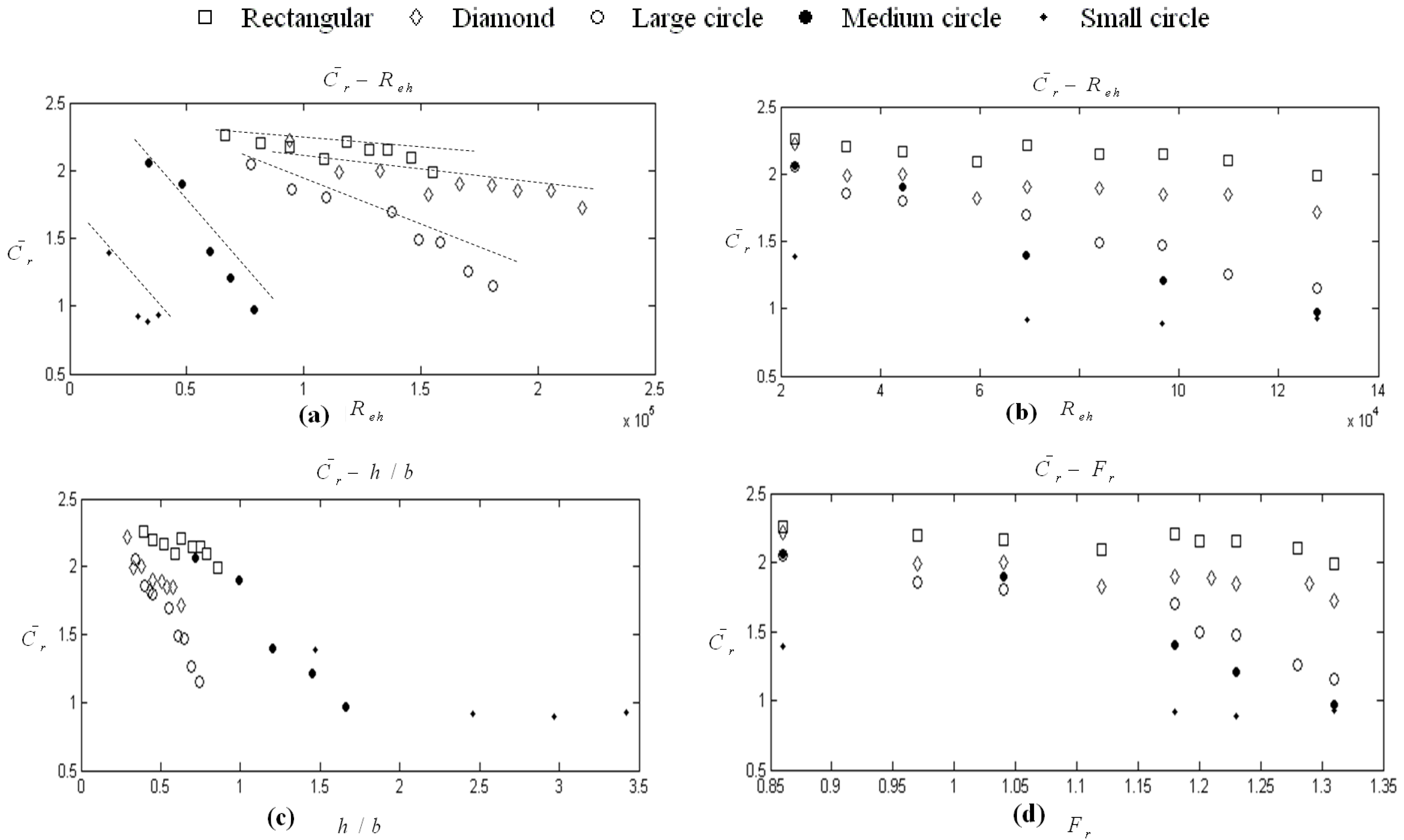
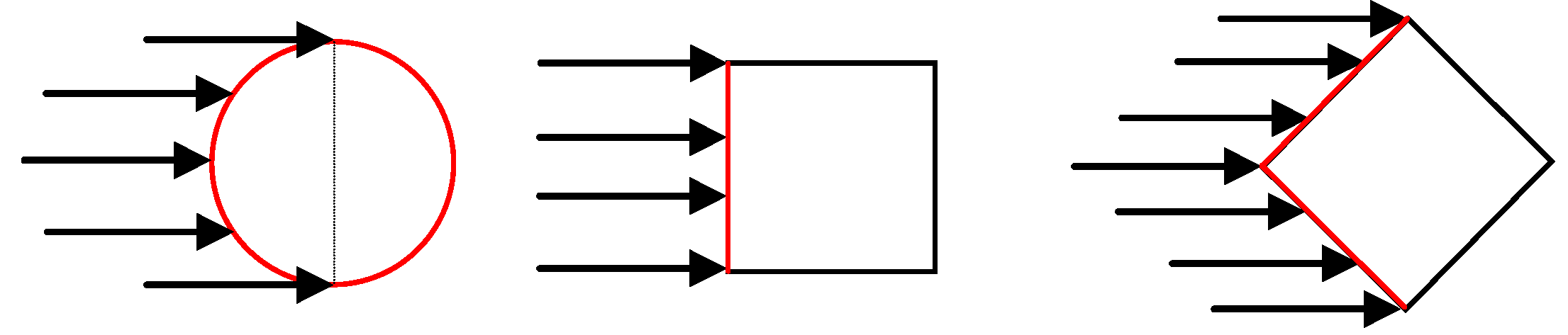
Yang et al. [1] also indicated is that there is no clear relationship between the variable and others such as R_eh, R_eb, F_r and h/b in Figure 2. However, it is quite obvious in Figure 2a and the others that there is a linear pattern between the obstacles of different shape and scale, which can be described in general as y = ax + b. Therefore, it is necessary to include a parameter that describes the shape of the obstacles. In this study, wide variety of combination is tried. It is seen that the perimeter of circle, one side length and two side lengths for rectangular and diamond obstacles, respectively, are found to be correlated with . This influence is described and proposed in this paper with a non-dimensional “shape of influence” parameter as w/h_o, where w is perimeter of circles, length of one side for rectangular and summation length of two sides for diamonds in Figure 3, and h_o is initial water depth as 20 mm.

The interrelation between and both h/b and the newly proposed variable w/h_o is investigated with linear regression models. The variable R_eh is excluded from the analysis for the sake of parsimoniousity because its influence is less, with magnitude of 1/3 compared to h/b. As a thumb rule, a linear model gives good results with normally distributed variables. Therefore, log-transformed variables were used for both h/b and w/h_o to regress. A stepwise linear regression procedure was employed. In the first step, log(h/b) was entered into the model by selection criteria that is mentioned in Section 4.3. As for the second step, log(w/h_o) was placed into the model. As shown in Table 8, all variables are statistically significant. In addition, adjusted R² value of the model increased to 0.86 as seen in Table 10. This is a satisfactory result when compared with the other models that are constructed in scope of this study. The collinearity diagnostics shows a tolerably collinearity problem, because the condition index is below 15 and VIF is smaller than 2 (Table 9). Therefore, new model is suggested which is in harmony with the regression assumptions as:

(14)

Figure 2. The variation of C_r (output) with relevant inputs.

Figure 2. The variation of C_r (output) with relevant inputs.

Figure 3. Proposed “shape of influence” parameter for structures.

Figure 3. Proposed “shape of influence” parameter for structures.

Table 9. The regression statistics of stepwise model.

Stepwise Model		Unstandardized Coefficients		Standardized Coefficients	t	Significance	Correlations	Partial	Part	Collinearity Statistics		Collinearity Diagnostics
		B	Std. Error	Beta			Zero order			Tolerance	VIF	Eigen value	Cond. Index
Step 1	Constant	1.55	0.05	–	29.48	0.00	–	–	–	–	–	1.51	1.00
Step 1	log(h/b)	−1.25	0.17	−0.78	−7.20	0.00	−0.78	−0.78	−0.78	1.00	1.00	0.49	1.75
Step 2	Constant	2.53	0.13	–	19.40	0.00	–	–	–	–	–	2.41	1.00
Step 2	log(h/b)	−1.74	0.12	−1.09	−14.28	0.00	−0.78	−0.93	−0.93	0.73	1.37	0.57	2.05
Step 2	log(w/ho)	−1.05	0.14	−0.59	−7.73	0.00	−0.02	−0.81	−0.50	0.73	1.37	0.02	10.88

Table 9. The regression statistics of stepwise model.

Stepwise Model		Unstandardized Coefficients		Standardized Coefficients	t	Significance	Correlations	Partial	Part	Collinearity Statistics		Collinearity Diagnostics
		B	Std. Error	Beta			Zero order			Tolerance	VIF	Eigen value	Cond. Index
Step 1	Constant	1.55	0.05	–	29.48	0.00	–	–	–	–	–	1.51	1.00
Step 1	log(h/b)	−1.25	0.17	−0.78	−7.20	0.00	−0.78	−0.78	−0.78	1.00	1.00	0.49	1.75
Step 2	Constant	2.53	0.13	–	19.40	0.00	–	–	–	–	–	2.41	1.00
Step 2	log(h/b)	−1.74	0.12	−1.09	−14.28	0.00	−0.78	−0.93	−0.93	0.73	1.37	0.57	2.05
Step 2	log(w/ho)	−1.05	0.14	−0.59	−7.73	0.00	−0.02	−0.81	−0.50	0.73	1.37	0.02	10.88

Table 10. Stepwise model summary statistics.

Model	R	R Square	Adjusted R Square	Std. Error of the Estimate	R Square Change	F Change		df1	df2	Sig. F Change
Step 1	0.782	0.61	0.60	0.27	0.61	51.84	1.00		33.00	0.00
step 2	0.930	0.86	0.86	0.16	0.25	59.79	1.00		32.00	0.00

Table 10. Stepwise model summary statistics.

Model	R	R Square	Adjusted R Square	Std. Error of the Estimate	R Square Change	F Change		df1	df2	Sig. F Change
Step 1	0.782	0.61	0.60	0.27	0.61	51.84	1.00		33.00	0.00
step 2	0.930	0.86	0.86	0.16	0.25	59.79	1.00		32.00	0.00

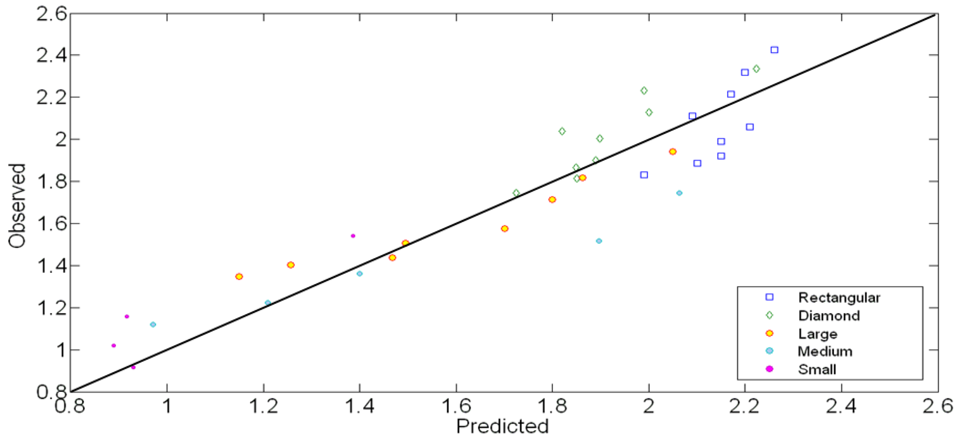
In order to test how the new proposed variable w/h_o can describe the “shape of influences” to the structures, triple diagram curves are plotted in Figure 4, in which all 35 data of [1] in Table 1 are employed. It is obvious that is highly dependent on these parameters. In addition, newly developed parameter w/h_o is capable of describing the behavior of in an efficient way. Contrary to the Figure 1, there are no any transitional zones dependent on obstacles in Figure 4 with proposed w/h_o variable. One can easily predict the by just inserting w/h_o and h/b on the figure, without describing the shape of structure in advance.

Figure 4. Distribution of with h/b and proposed w/h_o.

Figure 4. Distribution of with h/b and proposed w/h_o.

The regression assumption that mean of the average of residuals must be zero is checked in Figure 5. It is observed that the mean of the residuals is calculated as −0.0043, which meets the first criteria. The second check is performed for conditional distribution of the residuals that should be normally distributed. As seen in the Figure 6, the residuals abide normal distribution function with a significance level of 0.05 by using Kolmogrov–Smirnov test.

Figure 5. Residual behavior.

Figure 5. Residual behavior.

Figure 6. Normal probability plot.

Figure 6. Normal probability plot.

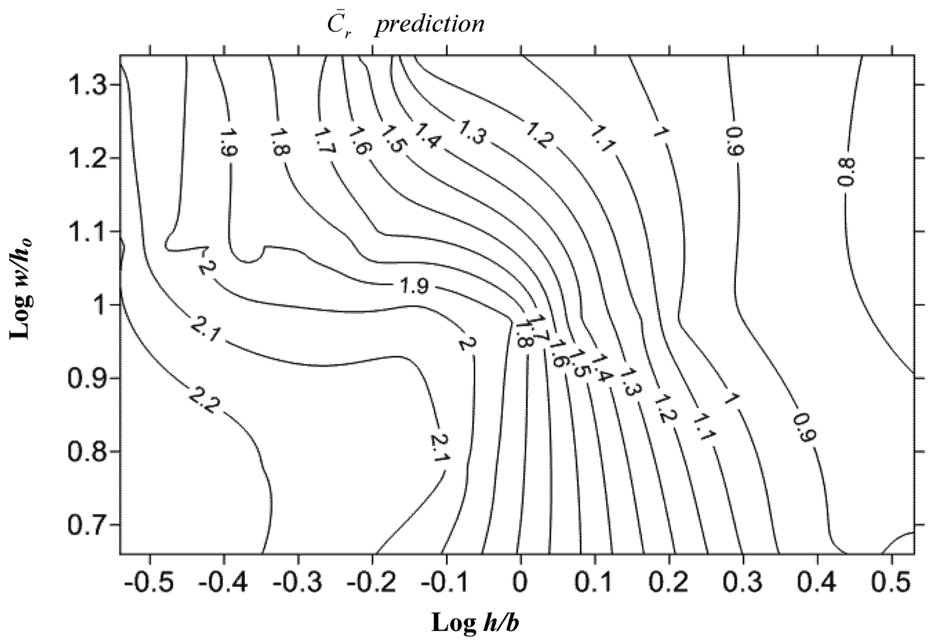
5. Evaluation of the Proposed Model for Mean Normalized Force Computation

The performance of the proposed model is achieved in terms of graphical representation and three different error statistics as mean absolute relative error (MARE), mean squared error (MSE) and coefficient of determination (R²). MARE and MSE indicate quantitative information of the model error with the characteristic that larger errors receive greater attention than smaller ones whereas R² demonstrates the measures of how much of the variation and trends in the observed data are predicted by the proposed model. The performance results of the proposed model for obstacles are given in Table 11.

Table 11. Performance of the proposed model for variety of obstacles.

Obstacle shape	Mean absolute relative error (MARE)	Mean squared error (MSE)	Coefficient of determination (R2)
Rectangular	0.0655	0.0241	0.5924
Diamond	0.0508	0.0165	0.7887
Large	0.0645	0.0123	0.9309
Medium	0.1086	0.0535	0.9563
Small	0.1339	0.0247	0.8522
Total	0.0755	0.0237	0.8643

Table 11. Performance of the proposed model for variety of obstacles.

Obstacle shape	Mean absolute relative error (MARE)	Mean squared error (MSE)	Coefficient of determination (R2)
Rectangular	0.0655	0.0241	0.5924
Diamond	0.0508	0.0165	0.7887
Large	0.0645	0.0123	0.9309
Medium	0.1086	0.0535	0.9563
Small	0.1339	0.0247	0.8522
Total	0.0755	0.0237	0.8643

As can be seen in Table 11, the minimum MARE occurs for diamond obstacle as 0.0508 whereas the maximum is as 0.1339 for small. In overall, it is 0.0755, which states that both obstacles follow each other very closely and the proposed variable w/h_o covers the influence of the obstacles in an efficient way. Based on MSE, both obstacles yield smaller prediction error. The overall prediction MSE is 0.0237. All obstacles yield similar results. As for R², the predictions are successful especially except the obstacle rectangular, which is lower than the others (Figure 7).

Figure 7. Scatter diagrams around perfect line for different types of obstacles.

Figure 7. Scatter diagrams around perfect line for different types of obstacles.

6. Conclusions

In this study, several statistical approaches as simple correlation analysis, multiple linear regression model, stepwise multiple linear regression model, principal component analysis and cluster analysis are employed to propose new and efficient formula. The regression model based on h/b and newly proposed parameter w/h_o is suggested to predict mean normalized force due to dam break. It is seen that the w/h_o parameter takes into account the shape of the obstacles in an appropriate way, which makes up parsimonious model in accordance with the engineering applications. The average MARE, MSE and R² values of the proposed model are 0.0755, 0.0237 and 0.8643, respectively. This demonstrates that the proposed model gives satisfactory results. In terms of coefficient of determination, only the rectangular obstacle gives lower prediction capability than others. Similar approaches can be applied for future research for predicting maximum forces on obstacles.

References

- Yang, C.; Lin, B.; Jiang, C.; Lin, Y. Predicting near-field dam break flow and impact force using 3D model. J. Hydraul. Res. 2010, 48, 784–792. [Google Scholar] [CrossRef]
- Chanson, H. The Hydraulics of Open Channel Flow: An Introduction, 2nd ed; Butterwort-Heinemann: Oxford, UK, 2004. [Google Scholar]
- Ritter, A. Die fortpflanzung der wasserwellen. Zeitschrift des Vereines Deutscher Ingenieure 1892, 36, 947–954. [Google Scholar]
- FEMA 55, Coastal Construction Manual, 3rd edFederal Emergency Management Agency: Jessup, MD, USA, 2003.
- Kaplan, P.; Murray, J.J.; Yu, W.C. Theoretical Analysis of Wave Impact Forces on Platform Deck Structures. In Proceedings of the Offshore Mechanics and Arctic Engineering Conference, OMAE Copenhagen, Denmark, 18–22 June 1995; 1A, pp. 353–374.
- Cumberbatch, E. The impact of water wedge on a wall. J. Fluid Mech. 1960, 7, 353–374. [Google Scholar] [CrossRef]
- Cross, R.H. Tsunami surge forces. J. Waterw. Harb. Div. ASCE 1967, 93, 201–231. [Google Scholar]
- Ramsden, J.D. Tsunamis: Forces on a Vertical Wall caused by Long Waves, Bores, and Surges on a Dry Bed. Ph.D. Thesis, California Institute of Technology, Pasadena, CA, USA, 1993. [Google Scholar]
- City and County of Honolulu Building Code (CCH); Chapter 16, Article 11; Department of Planning and Permitting of Honolulu: Honolulu, HI, USA, 2000.
- Dames and Moore. In Design and Construction Standards for residential Construction in Tsunami Prone Areas in Hawaii; Prepared for Federal Emergency Management Agency: Washington, DC, USA, 1980.
- Mikhaylov, Y.; Robertson, I.N. Evaluation of Prototypical Reinforced Concrete Building Performance when Subjected to Tsunami Loading; Research Report UHM/CEE/09-01; Sage Publications: New Delhi, India, 2009. [Google Scholar]
- Soares-Frazão, S. Experiments of dam-break wave over triangular bottom sill. J. Hydraul. Res. 2007, 45, 9–26. [Google Scholar] [CrossRef]
- Miller, S.; Chaudhry, M.H. Dam-break flows in curved channel. J. Hydraul. Eng. ASCE 1989, 115, 1465–1478. [Google Scholar] [CrossRef]
- Cagatay, H.; Kocaman, S. Experimental study of tail water level effects on dam-break flood wave propagation. In Proceedings of River Flow Conference, Cesme, Turkey, 3–5 September 2008; 1, pp. 635–644.
- Aureli, F.; Maranzoni, A.; Mignosa, P.; Ziveri, C. Dam-break flows: Acquisition of experimental data through an imaging technique and 2D numerical modelling. J. Hydraul. Eng. ASCE 2008, 134, 1089–1101. [Google Scholar] [CrossRef]
- Oertel, M.; Bung, D.B. Initial stage of two-dimensional dam-break waves: Laboratory versus VOF. J. Hydraul. Res. 2012, 50, 89–97. [Google Scholar] [CrossRef]
- Soares-Frazão, S.; Zech, Y. Dam-break in channels with 90-degree bend. J. Hydraul. Res. 2002, 128, 956–968. [Google Scholar] [CrossRef]
- Chanson, H. Application of the method of characteristics to the dam break wave problem. J. Hydraul. Res. 2009, 1, 41–49. [Google Scholar] [CrossRef]
- Arnason, H. Interactions between Incident Bore and a Free-Standing Coastal Structure. Ph.D. Thesis, University of Washington, Seattle, WA, USA, 2005. [Google Scholar]
- Arnason, H.; Petroff, C.; Yeh, H. Tsunami bore impingement onto a vertical column. J. Disaster Res. 2009, 4, 391–403. [Google Scholar]
- Yeh, H.; Ghazali, A.; Marton, I. Experimental study of bore run-up. J. Fluid Mech. 1989, 206, 563–578. [Google Scholar] [CrossRef]
© 2013 by the authors; licensee MDPI, Basel, Switzerland. This article is an open access article distributed under the terms and conditions of the Creative Commons Attribution license (http://creativecommons.org/licenses/by/3.0/).
Share and Cite
Duricic, J.; Erdik, T.; Pektaş, A.O.; Van Gelder, P.H.A.J.M. Mean Normalized Force Computation for Different Types of Obstacles due to Dam Break Using Statistical Techniques. Water 2013, 5, 560-577. https://doi.org/10.3390/w5020560
Duricic J, Erdik T, Pektaş AO, Van Gelder PHAJM. Mean Normalized Force Computation for Different Types of Obstacles due to Dam Break Using Statistical Techniques. Water. 2013; 5(2):560-577. https://doi.org/10.3390/w5020560
Chicago/Turabian StyleDuricic, Jasna, Tarkan Erdik, Ali Osman Pektaş, and Petrus H.A.J.M Van Gelder. 2013. "Mean Normalized Force Computation for Different Types of Obstacles due to Dam Break Using Statistical Techniques" Water 5, no. 2: 560-577. https://doi.org/10.3390/w5020560
APA StyleDuricic, J., Erdik, T., Pektaş, A. O., & Van Gelder, P. H. A. J. M. (2013). Mean Normalized Force Computation for Different Types of Obstacles due to Dam Break Using Statistical Techniques. Water, 5(2), 560-577. https://doi.org/10.3390/w5020560