Remote Sensing and U-Net-Based Prediction of Cyanobacterial Bloom Responses to Warming in Lake Taihu

Abstract

In view of the limitations of existing studies, in which remote sensing extraction of algal blooms is easily affected by cloud interference, and mechanistic models are constrained by excessive parameters and inadequate representation of nonlinear relationships, resulting in limited timeliness and accuracy, this study took Taihu Lake as the study area and constructed a research framework of bloom extraction-scale matching-spatial prediction-scenario response based on Landsat imagery and gridded meteorological data, constructing the relationship between meteorological factors and algal blooms using machine learning methods. First, the Tasseled Cap transformation (TCap) and Floating Algae Index (FAI) were combined to extract the spatial distribution and area of algal blooms, while cloud interference was addressed to improve recognition stability under complex background conditions. Next, the spatial scales of bloom rasters and meteorological factors were unified to build a matched bloom-meteorological dataset. On this basis, a U-Net model driven by multiple meteorological factors was developed to predict remote-sensing-based bloom distribution/extent patterns under three warming scenarios. The results showed that: (1) the combination of TCap and FAI improved the accuracy and efficiency of bloom extraction; FAI was more sensitive but tended to overestimate bloom area, whereas TCap was more stable under cloud interference; (2) the U-Net model achieved an overall accuracy of 95% and a prediction accuracy of 88%; and (3) bloom area increased under all three warming scenarios, and the extent of expansion generally became more pronounced with increasing warming magnitude, although the response was not strictly monotonic across all cases. Based on the seasonal mean bloom-area increase relative to the baseline condition (S0), the warming response was strongest in spring, followed by summer and autumn, and weakest in winter. This study can provide a reference for cyanobacterial bloom early warning and water environment management in Lake Taihu.

1. Introduction

Lake ecosystems are among the most important sources of drinking water and freshwater resources worldwide. However, with accelerating industrialization, urbanization, and modernization, eutrophication in freshwater lakes has become increasingly severe, resulting in ecological degradation, reduced water availability, and deteriorated water quality, and thereby posing serious environmental, economic, and social threats [1,2,3,4,5]. Eutrophication is originally a natural process driven by the gradual accumulation of nutrients such as nitrogen and phosphorus in the water column and sediments [6]. Since the mid-20th century, however, human activities have greatly accelerated this process, causing many lakes to shift rapidly to eutrophic conditions. Cyanobacterial blooms are one of the most typical manifestations of eutrophication, and their frequency and extent have increased worldwide. Therefore, effective prediction of cyanobacterial blooms is of great importance for lake management.

Remote sensing has shown strong potential for cyanobacterial bloom monitoring, water environment assessment, and ecosystem health evaluation. With advances in high-resolution imagery and data-processing techniques, it has become an important tool for water environment management. For example, the ground-based remote sensing approach proposed by Zhang et al., combined with hyperspectral imaging and artificial intelligence algorithms, enables high-frequency and accurate monitoring of water quality parameters [7]. In addition, remote sensing provides abundant data support for bloom monitoring [8]. Commonly used spectral indices include band ratio indices [9], normalized difference vegetation index (NDVI) [10], maximum chlorophyll index (MCI) [11], and floating algae index (FAI) [12]. Among them, FAI is less affected by aerosol scattering in the near-infrared and red bands, making it more suitable for bloom area extraction [13]. Compared with conventional field surveys, remote sensing methods based on MODIS and Landsat 8 imagery can identify and quantify bloom distribution more efficiently at the lake scale.

Nevertheless, cloud contamination remains a major limitation for remote sensing applications. Existing studies have mainly addressed this issue through cloud detection and cloud-pixel reconstruction. Zhu and Woodcock developed the Fmask algorithm for accurate cloud and cloud-shadow detection in Landsat imagery [14]. Louis et al., used the scene classification layer and quality bands of Sentinel-2 L2A products to dynamically identify and fill cloud-contaminated pixels [15], while Li et al. further introduced deep learning methods for cloud detection and cloud-removal reconstruction [16]. In China, Zhang Chengyao proposed a detection–fusion–reconstruction framework for cloud and shadow removal with high-fidelity image recovery [17], and Wen et al., developed a cloud-snow detection method integrating spatiotemporal information to improve recognition accuracy [18]. Overall, cloud-processing methods have evolved from threshold-based approaches to multi-source fusion and deep learning frameworks, but their application in lake bloom detection remains limited and the workflow is still relatively complex.

Climatic factors can influence lake ecosystem structure and function by altering lake heat balance and water mixing processes. Although many previous studies have focused on water quality and aquatic ecological simulations, studies predicting cyanobacterial blooms based mainly on meteorological drivers remain limited. In particular, when multi-source datasets differ in spatial resolution, temporal scale, and data format, building a unified data framework for future scenario prediction remains a major challenge. Therefore, this study focuses on Lake Taihu and investigates cyanobacterial bloom extraction and meteorological driver-based prediction, with the aim of providing methodological support and scientific reference for eutrophication control under climate warming.

2. Materials and Methods

2.1. Study Area

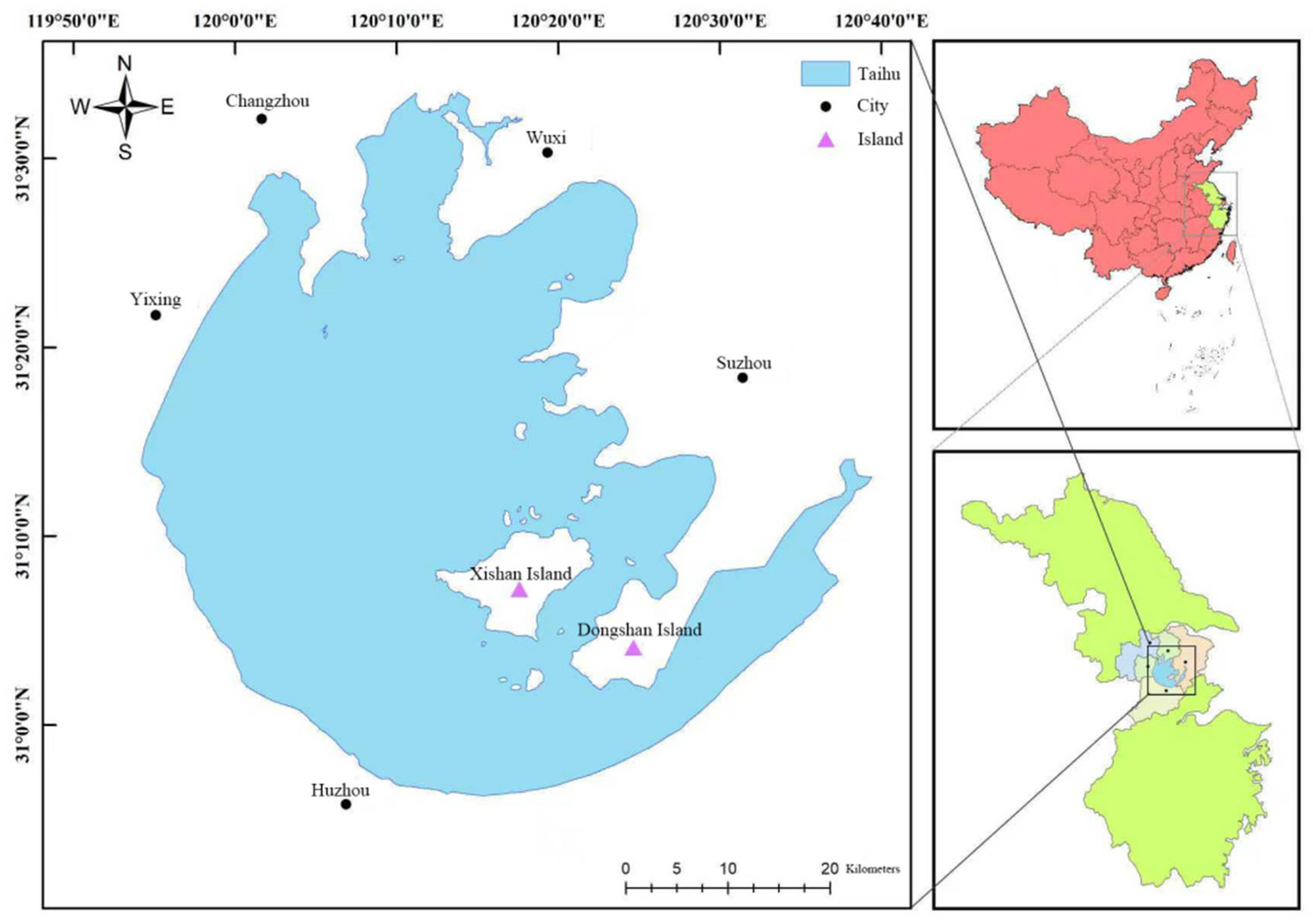
Lake Taihu (Figure 1) (30°5′–32°8′ N, 119°8′–121°55′ E) is located in southern Jiangsu Province, adjacent to Zhejiang Province, and is the third-largest freshwater lake in China. It has a water surface elevation of 3.33 m, a mean water depth of 1.9 m, and a surface area of 2338 km². The western and southwestern parts of the basin are characterized by hills and low mountains, whereas the eastern part is dominated by plains and dense river networks. Owing to the long-term influence of eutrophication, cyanobacterial blooms in summer have exerted pronounced impacts on water quality and aquatic ecosystems. Given its geographical importance and ecological functions, Lake Taihu has become a key region for national water-resource management and environmental protection. Over the past decade (2015–2024), bloom intensity was generally higher during 2016–2020, with an exceptionally severe outbreak in 2017, followed by a rapid decline during 2021–2023. In 2023, the annual mean bloom area decreased to 77 km² and the cumulative bloom area was 2693 km², representing the lowest levels since 2003. In 2024, cyanobacterial bloom occurrence frequency was ≤10 times across most areas of the lake, while localized regions in the western lake exceeded 15 occurrences [19].

2.2. Data Acquisition and Processing

In this study, Landsat 8 surface reflectance data from 2013 to 2025 were acquired through the Google Earth Engine (GEE) cloud platform. These data had already undergone radiometric calibration and atmospheric correction on the platform and could therefore be used directly for cyanobacterial bloom monitoring. Using the Lake Taihu boundary vector dataset for spatial masking, the imagery was further processed by band normalization, and multiple scenes acquired on the same date were mosaicked. The processed images were then exported as GeoTIFF files with a spatial resolution of 30 m in the WGS84/UTM projection, for subsequent offline index calculation and spatiotemporal analysis. This workflow ensured stable quality of the time-series data and minimized atmospheric and other sources of interference, thereby providing a reliable data foundation for subsequent extraction of bloom-related indices, such as FAI, and for statistical modeling. The meteorological data used in this study were obtained from the fifth-generation atmospheric reanalysis dataset ERA5, released by the European Centre for Medium-Range Weather Forecasts (ECMWF) and provided through the Copernicus Climate Data Store. From the ERA5 gridded products, variables closely related to hydrological processes were extracted, including 2 m air temperature, 10 m u- and v-wind components (from which wind speed and wind direction can be derived), surface solar radiation downwards (SSRD), total precipitation (tp), and evaporation (e/ET).

2.3. Research Methods

2.3.1. Floating Algae Index (FAI)

The FAI combines reflectance information from the red, near-infrared (NIR), and shortwave-infrared (SWIR) bands, and can effectively discriminate open water from floating cyanobacterial scums. Compared with commonly used vegetation indices such as NDVI or EVI, FAI is less sensitive to environmental factors including aerosol type and loading, sun glint, and viewing/illumination geometry, and thus provides higher stability for long-term bloom monitoring in freshwater lakes. FAI is calculated as(1):

$$\mathit{FAI} ={\mathit{R}}_{\mathit{rc},\mathit{NIR}}-{\mathit{R}}_{\mathit{rc},\mathit{Red}}-\left({\mathit{R}}_{\mathit{rc},\mathit{SWIR}}-{\mathit{R}}_{\mathit{rc},\mathit{Red}}\right)·{\displaystyle \frac{{\mathsf{\lambda }}_{\mathit{NIR}}-{\mathsf{\lambda }}_{\mathit{Red}}}{{\mathsf{\lambda }}_{\mathit{SWIR}}-{\mathsf{\lambda }}_{\mathit{Red}}}}$$

(1)

where ${\mathit{R}}_{\mathit{rc},\mathit{Red}}$, ${\mathit{R}}_{\mathit{rc},\mathit{NIR}}$, ${\mathit{R}}_{\mathit{rc},\mathit{SWIR}}$ are the atmospherically corrected surface reflectance in the red, NIR, and SWIR bands, respectively; ${\mathsf{\lambda }}_{\mathit{Red}}$, ${\mathsf{\lambda }}_{\mathit{NIR}}$, ${\mathsf{\lambda }}_{\mathit{SWIR}}$ denote the corresponding central wavelengths, set to 655 nm, 865 nm, and 1610 nm, respectively.

For each FAI image, a gradient image can be generated to aid adaptive thresholding. The pixel-wise gradient is defined as the FAI difference between adjacent pixels within a 3 × 3 window [20]. Because high concentrations of suspended matter in water can interfere with cyanobacterial bloom extraction, an initial threshold was applied to separate such contaminated pixels. Gradient values were then computed for the remaining pixels. Previous studies indicate that the FAI value associated with the maximum gradient can be used to distinguish phytoplankton (bloom) pixels from pure-water pixels. After automatically deriving FAI for each Landsat image, an image-specific algae threshold was determined from the histogram of gradient distribution based on the summed FAI differences within the 3 × 3 neighborhood. Following this procedure, a non-algal pixel threshold was set to −0.004 by subtracting twice the standard deviation from the mean threshold across all images [21,22].

2.3.2. Tasseled Cap Transformation

Existing methods for cyanobacterial bloom identification are prone to misclassifying cloud pixels as blooms and rely heavily on atmospheric correction. Inappropriate correction may introduce substantial errors and often requires extensive field measurements to reduce monitoring uncertainty [23]. By contrast, the tasseled cap transformation can highlight cyanobacterial bloom features and suppress cloud and haze interference without requiring atmospheric correction, thereby greatly simplifying the extraction procedure. On this basis, a novel cyanobacterial bloom extraction model based on TCap was developed.

The tasseled cap transformation (also known as the K–T transformation), first proposed by Kauth and Thomas in 1996, is a linear orthogonal transformation derived from principal component analysis [24]. It not only compresses multispectral image information but also enhances the red-edge signal of vegetation, and was originally developed for terrestrial vegetation extraction [25,26]. Cyanobacteria floating on the water surface likewise exhibit a pronounced red-edge characteristic. After tasseled cap transformation, they can be effectively distinguished from surrounding water, and cloud interference can be further reduced through combinations of different transformed components. This method has been validated using imagery from Landsat-8, QuickBird, MODIS, and HJ-1 sensors. Using the tasseled cap coefficients for the Landsat-8 OLI sensor, the transformation is expressed as Equation (2):

$$\left(\begin{array}{c}\mathit{TGG}\\ \mathit{TCB}\\ \mathit{TCW}\\ \mathit{TCN}\end{array}\right)=\left(\begin{array}{cccc}0.3521& 0.3899& 0.3825& 0.6985\\ -0.3301& -0.3455& -0.4508& 0.6970\\ 0.2651& 0.2361& 0.1296& 0.0590\\ 0.1010& -0.0507& 0.1964& -0.1239\end{array} \right)*\left(\begin{array}{c}{\mathit{DN}}_{\mathit{b}}\\ {\mathit{DN}}_{\mathit{g}}\\ {\mathit{DN}}_{\mathit{r}}\\ {\mathit{DN}}_{\mathit{n}}\end{array}\right)$$

(2)

where TCG, TCB, TCW, and TCN denote greenness, brightness, wetness, and the orthogonal component, respectively; and DN_b, DN_g, DN_r, and DN_n represent the reflectance values of the blue, green, red, and near-infrared bands, respectively.

To address the limitation of existing indices that frequently misclassify clouds and cloud edges as cyanobacterial blooms, a sample library containing cyanobacterial blooms, water bodies, and clouds was constructed based on Landsat imagery. Nine representative images capturing bloom outbreaks in Lake Taihu during different periods from 2017 to 2020 were selected and divided into training and testing datasets. Among them, water, cloud, and cloud-edge pixels were labeled through visual interpretation, whereas bloom samples were extracted using an FAI threshold of −0.004 in combination with green pixels identified from false-color composites. A total of 4 × 10⁴ pixels were selected as samples.

In this study, to comprehensively evaluate the classification performance of the bloom-identification model, samples were categorized on the basis of a pixel-level confusion matrix into four groups: true positives (TP), false positives (FP), false negatives (FN), and true negatives (TN). To achieve a balance between precision and recall, the F1 score was calculated as their harmonic mean(3):

$$\mathit{F}1 = 2 * {\displaystyle \frac{\mathit{precision} * \mathit{recall}}{\mathit{precision}+\mathit{recall}}}$$

(3)

Using cyanobacterial bloom, water, and cloud pixels from the training dataset, the model evaluated the capability of the TCap method for bloom extraction. For each pixel, four transformed components (TCB, TCG, TCW, and TCN) were calculated. To integrate the strengths of these components, new composite variables were generated using linear combinations with coefficients of −1, 0, and 1, yielding a total of 81 possible combinations. Their values were calculated for the training dataset, and the optimal combination and threshold were selected according to the F1 score. Based on model computation and extensive out-of-sample experiments, the optimal threshold was determined to be −0.015, and the component combination with the highest F1 score was identified as I = TCG − TCN, with an F1 score of 97%.

The following metrics were used to compare the relative error and coefficient of determination (R²) of the two models in estimating cyanobacterial bloom area and spatial distribution in Lake Taihu under clear-sky conditions. The corresponding equations are as follows:

The following metrics were used to compare, under clear-sky conditions, the relative bias in cyanobacterial bloom area estimated by the two models across Lake Taihu and among subregions, as well as the coefficient of determination (R²). The corresponding formulas are given below (4)–(6):

$${\mathit{R}}^2=1-{\displaystyle \frac{\sum _{\mathit{i}=1}^{\mathit{n}}\left({\mathit{y}}_{\mathit{F},\mathit{i}}-{\mathit{y}}_{\mathit{Y},\mathit{i}}\right)2}{\sum _{\mathit{i}=1}^{\mathit{n}}\left({\mathit{y}}_{\mathit{F},\mathit{i}}-{\stackrel{-}{\mathit{y}}}_{\mathit{F},\mathit{i}}\right)2}}$$

(4)

$$\mathit{ARE}={\displaystyle \frac{\left|{\mathit{x}}_{\mathit{F},\mathit{i}}{-\mathit{x}}_{\mathit{Y},\mathit{i}}\right|}{{\mathit{x}}_{\mathit{F},\mathit{i}}}} * 100\%$$

(5)

$$\mathrm{N}\mathit{RMSE}={\displaystyle \frac{\sqrt{\frac{{\sum }_{\mathit{i}=1}^{\mathit{n}}{\left({\mathit{X}}_{\mathit{F},\mathit{i}}-{\mathit{Y}}_{\mathit{F},\mathit{i}}\right)}^2}{\mathit{n}}}}{Ȳ}}$$

(6)

where x_F and x_Y denote the bloom areas extracted using the FAI-based method and the TCap-based method, respectively, and N is the number of samples.

2.3.3. U-Net

U-Net is a classical convolutional neural network architecture for image segmentation, originally proposed by Ronneberger et al. in 2015 [27]. Featuring a symmetric encoder–decoder structure and skip-connection mechanism, it can effectively integrate high-level semantic information with shallow fine-scale features, and thus achieves relatively high segmentation accuracy even under limited-sample conditions [27]. Its general workflow includes input data preprocessing and augmentation, multi-scale feature extraction through downsampling in the encoder, recovery of spatial information through upsampling and feature concatenation in the decoder, and final generation of a pixel-level probability map, followed by training and evaluation using loss functions such as cross-entropy and Dice loss.

For convolution and feature mapping, a two-dimensional convolution is applied to the input feature map x (including channel dimension c). Taking the k-th output channel as an example:

$${\mathit{y}}_{\mathit{k}}(\mathit{i},\mathit{j}) =\sum _{\mathit{c}}\sum _{\mathit{u}}\sum _{\mathit{v}}{\mathit{w}}_{\mathit{k},\mathit{c}}(\mathit{u},\mathit{v}){\mathit{x}}_{\mathit{c}}(\mathit{i}+\mathit{u},\mathit{j}+\mathit{v})+{\mathit{b}}_{\mathit{k}}$$

(7)

For upsampling in the decoder and skip connections, the decoding path commonly employs transposed convolution or interpolation-based upsampling. Denoting the upsampling operation as Up(·), the feature representation at the l-th decoding layer can be expressed as follows:

$${\mathit{x}}^{\mathit{l}} = {\mathit{U}}_{\mathit{p}}({\mathit{x}}_{\mathit{dec}}^{(\mathit{l}+1)})$$

(8)

It is then concatenated along the channel dimension (concat) with the encoder feature ${\mathit{x}}_{\mathit{enc}}^{\mathit{l}}$ at the corresponding scale:

$${\mathit{z}}^{\left(\mathit{l}\right)} =\mathit{Concat}({\mathit{x}}^{\mathit{l}},{\mathit{x}}_{\mathit{enc}}^{\mathit{l}})$$

(9)

It is subsequently passed through a convolutional block to obtain the fused feature ${\mathit{x}}_{\mathit{enc}}^{\mathit{l}}$. This integration of semantic information and fine-scale details is the key to the boundary refinement capability of U-Net.

Loss functions (original U-Net and commonly used variants):For the pixel-wise cross-entropy loss, the multi-class pixel-level cross-entropy can be written as follows:

$${\mathit{L}}_{\mathit{CE}} = -\sum _{\mathit{i}}{\sum }_{\mathit{c}=1}^{\mathit{C}}{\mathit{y}}_{\mathit{i},\mathit{c}}\mathit{log}({\mathit{p}}_{\mathit{i},\mathit{c}})$$

(10)

where ${\mathit{y}}_{\mathit{i},\mathit{c}}$ is the one-hot encoded ground-truth label.

3. Results

3.1. Bloom Area and Spatial Distribution of Cyanobacterial Outbreaks

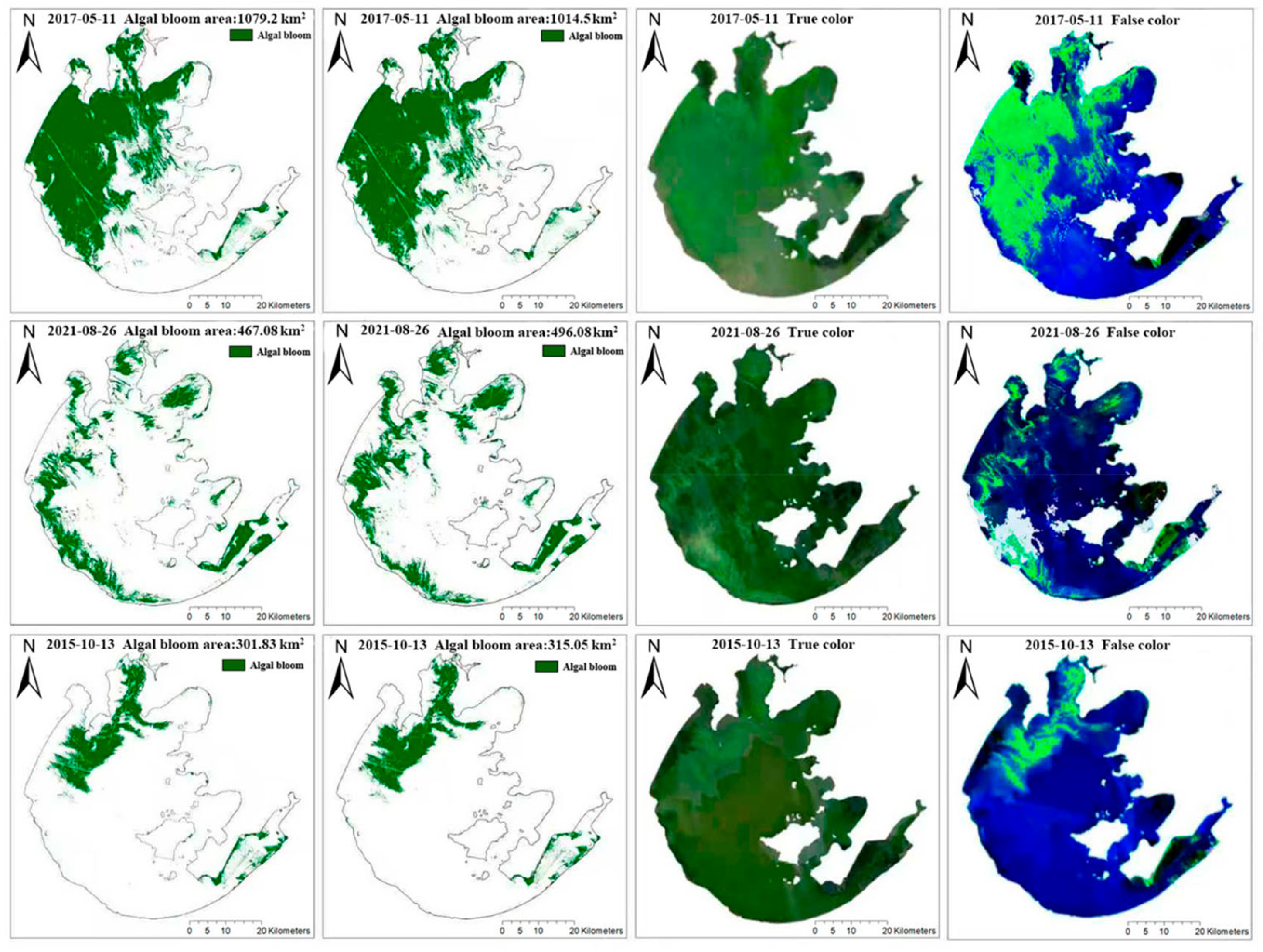
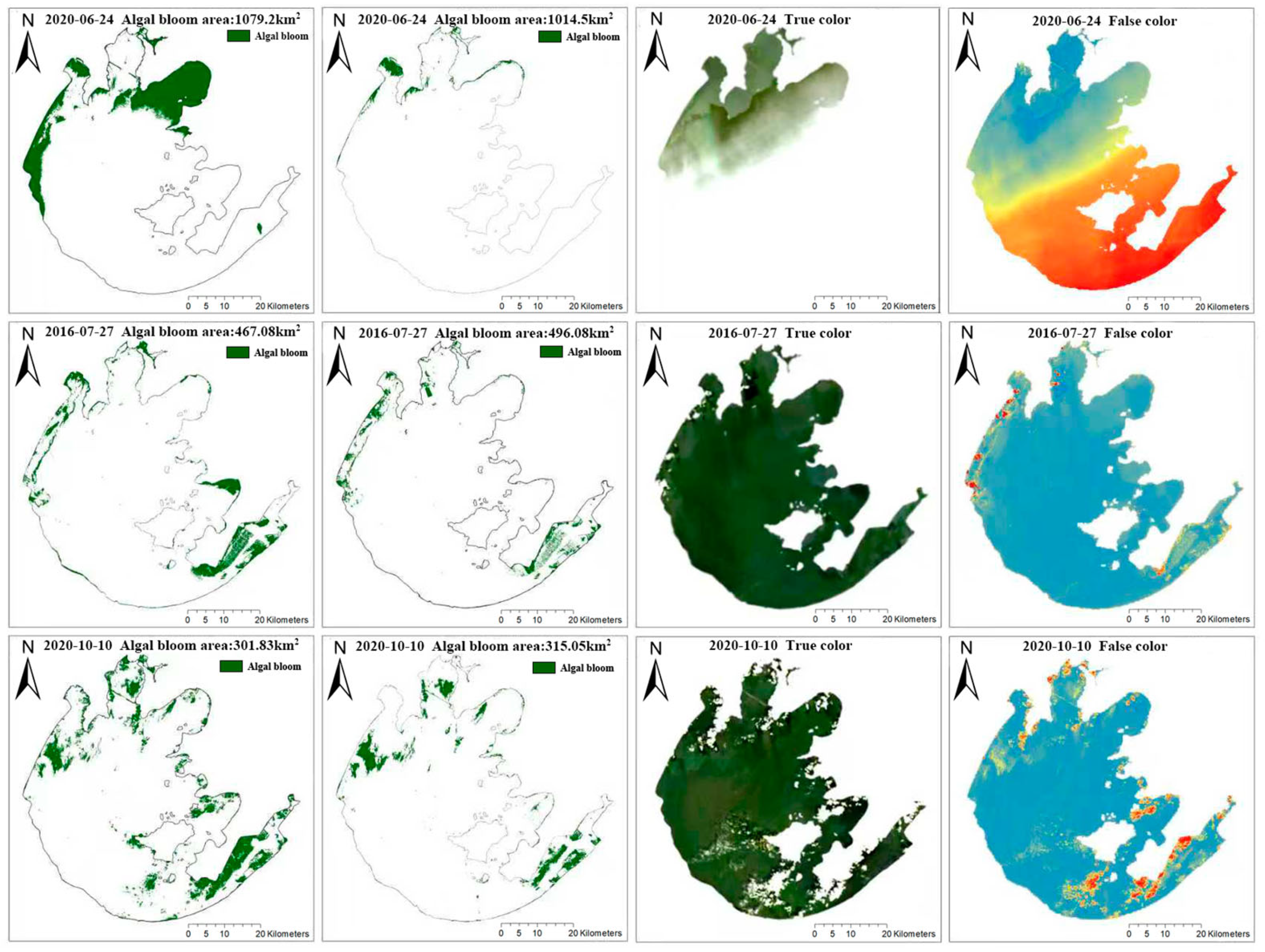
After preprocessing, the remote sensing data were used to estimate the cyanobacterial bloom area in Lake Taihu using the FAI and TCap methods, respectively. In the figures, the spatial distribution of blooms is marked in green (only selected representative examples are shown; the first column presents the FAI results, the second column the TCap results, the third column the true-color images, and the fourth column the false-color composites). The proportion of bloom-covered areas was visually interpreted from the RGB images, and the FAI- and TCap-derived results were compared against these visually interpreted reference patterns. This comparison was intended as a relative image-based benchmark for spatial consistency and cloud-related misclassification, rather than as an independent ecological validation. It should be noted that, because synchronous in situ measurements of chlorophyll-a, phycocyanin, or cyanobacterial cell counts were not available for the full image time series, the present evaluation focused on remote-sensing pattern consistency rather than independent biomass validation. Therefore, the estimated bloom extent should be interpreted as a remote-sensing-derived surface-bloom proxy rather than a direct measure of cyanobacterial biomass or cell abundance.

Late spring to early summer is the main outbreak period for cyanobacterial blooms in Lake Taihu. Rising temperature accelerates cyanobacterial growth and enhances its competitive advantage, while strong radiation and thermal stratification favor its persistence in surface waters. At the same time, agricultural runoff, domestic sewage, and sediment release promote nitrogen and phosphorus accumulation, and low wind speed with weak mixing further facilitates bloom aggregation, jointly triggering large-scale outbreaks. Water temperature in May is typically close to 20 °C, which is highly favorable for rapid cyanobacterial proliferation. As shown in Figure 2, bloom areas in periods b and c were 496.08 km² and 315.05 km², respectively, whereas period a reached 1000 km², indicating a severe bloom event. This may be related to substantially higher precipitation and post-rainfall conditions with low cloud cover and weak wind, which enhanced nutrient input and surface-water stability. All images were acquired under clear-sky conditions (cloud cover < 10%), and the bloom patterns were highly consistent between true-color and false-color images, indicating that the Landsat + FAI/TCap approach performs well under clear-sky conditions. Spatially, blooms were mainly concentrated in Meiliang Bay in the northwest and, under severe conditions, could expand to the western and central lake regions, while the eastern bay may be slightly overestimated due to persistent phytoplankton accumulation.

In the false-color composites, cloud-covered areas can be readily distinguished by their markedly darker reflectance, appearing as red, dark yellow, and part of the light-yellow regions (thin clouds), whereas the remaining yellow areas correspond to cyanobacterial blooms. These features were interpreted in conjunction with the true-color images for comparison. As clearly shown in Figure 3, the proposed model effectively removes cloud interference and extracts only bloom areas within the lake. This is particularly evident in panel d, where approximately two-thirds of the true-color image is obscured by clouds. Nevertheless, the model completely excluded the cloud-covered regions while accurately identifying the bright green bloom patches, which correspond to the yellow area in the upper-left portion of the false-color image. Similar results were obtained for the other two dates: although parts of the images were also affected by cloud cover, these cloud-contaminated regions were not misidentified as blooms, whereas the limited bright green patches were all correctly extracted as bloom areas, consistent with the corresponding yellow regions in the false-color composites. These results demonstrate that the TCap model shows strong adaptability in both accurate bloom identification and cloud removal. By comparison, the bloom areas derived from FAI were consistently larger than those from TCap, because FAI tended to misclassify some thin clouds as blooms, thereby resulting in overestimation.

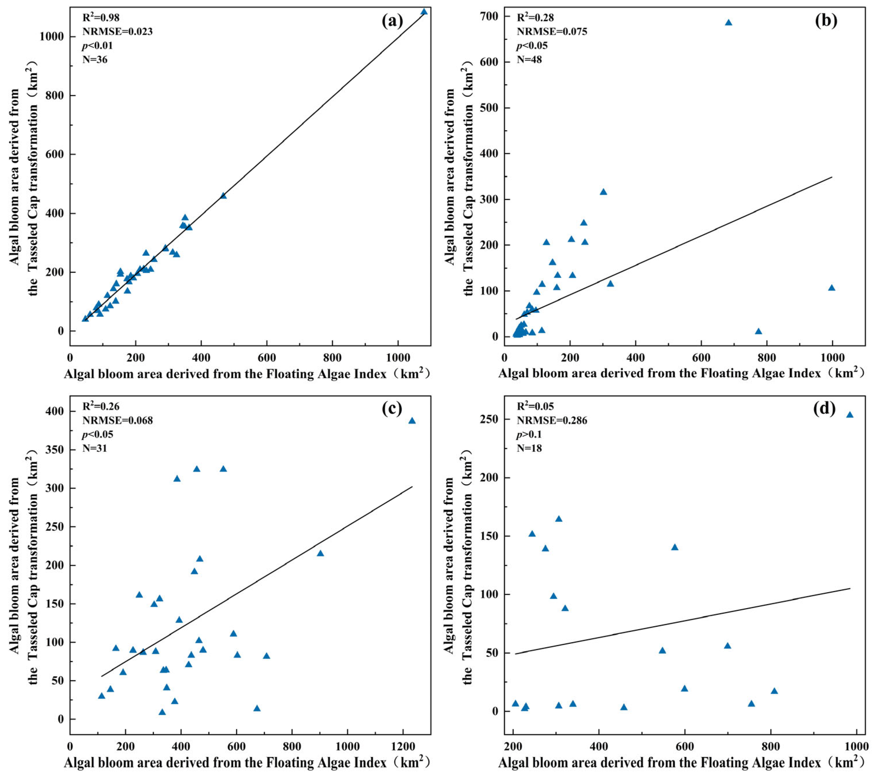
As shown in Figure 4, the bloom areas extracted by FAI and TCap were generally positively correlated, but their consistency varied markedly across different periods and cloud conditions. Under clear-sky conditions during the high-bloom period (April–September), the two methods showed the highest agreement, with scatter points closely distributed around the 1:1 line (R² = 0.98, p < 0.01; NRMSE = 0.023). In contrast, during the clear-sky low-bloom period (October–March), the agreement declined substantially (R² = 0.28; NRMSE = 0.075), and FAI generally produced higher estimates than TCap, possibly due to the fragmented distribution of blooms and background brightness effects. Under cloudy conditions, the consistency further weakened: only a moderate correlation was observed during the high-bloom period (R² = 0.26; NRMSE = 0.068), with TCap tending to underestimate bloom area when blooms were extensive, whereas the weakest agreement occurred during the low-bloom period (R² = 0.05; NRMSE = 0.286), with almost no clear linear relationship. These results indicate that the consistency between FAI and TCap gradually decreased as bloom intensity weakened and distribution conditions became more complex. Overall, the two methods were highly consistent when bloom coverage was extensive and the water signal was strong, but differed substantially when blooms were sparse or water conditions were more mixed.

3.2. Analysis of U-Net Model Results

In this study, multi-source meteorological driving factors were subjected to Kriging-based spatial interpolation and raster reconstruction in order to unify their spatial resolution, projection coordinate system, and raster cell attributes, thereby constructing a continuous meteorological feature dataset that satisfied the input requirements of the model. In addition, the bloom rasters extracted from remote sensing imagery were processed through scale conversion and binarization. By means of spatial aggregation, resampling, and threshold-based classification, the original bloom information was transformed into a binary response variable representing bloom occurrence status. On this basis, the meteorological factor rasters and bloom binary rasters were further aligned precisely in terms of spatial extent, resolution, and pixel correspondence, thereby generating coupled meteorological–bloom input samples that could be directly used for model training and prediction.

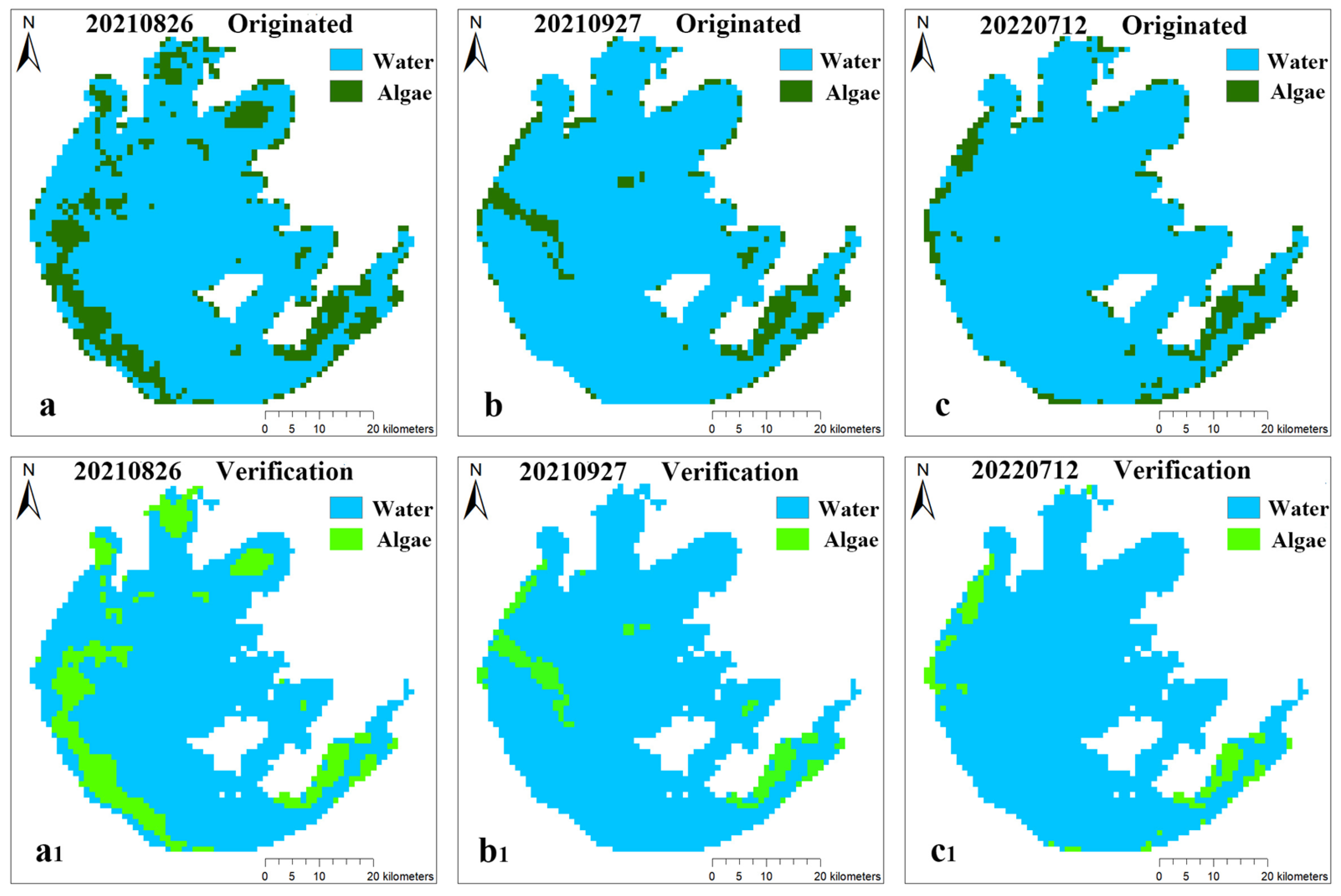
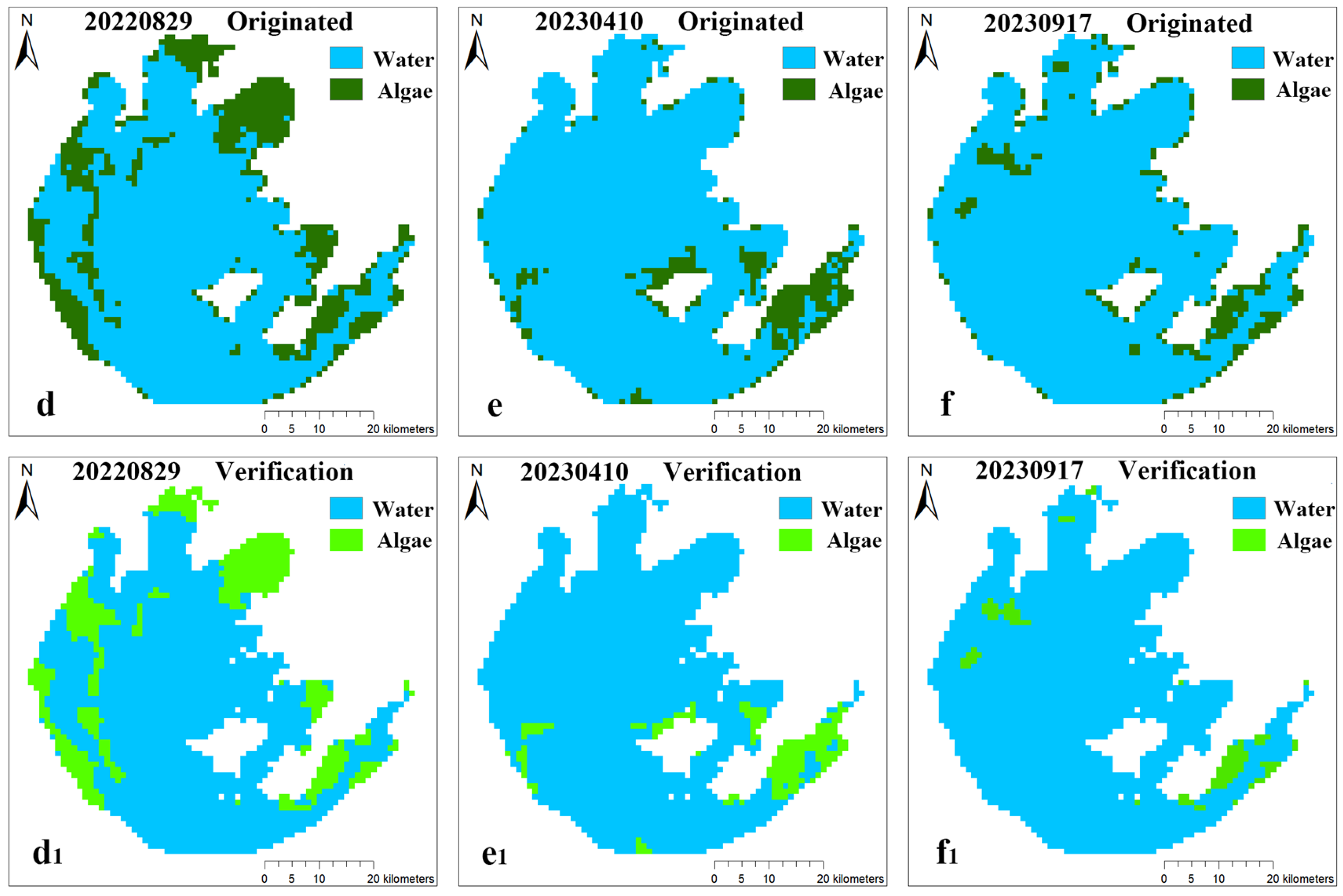
As shown in Figure 5, the spatial distribution of algal blooms in the validation samples was generally consistent across different dates, indicating that the model had a good capability to capture the relationship between meteorological factors and bloom occurrence. Overall, the predicted results clearly identified the main bloom aggregation areas in Lake Taihu, particularly in littoral zones, bays, and relatively enclosed waters, suggesting that the model successfully extracted the key features closely associated with bloom development and produced a relatively stable spatial representation in the validation set. In general, the model showed reliable performance in identifying the large-scale bloom pattern and major hotspot locations, with more stable predictions for bloom events characterized by larger area and stronger aggregation. However, its performance remained limited in representing local boundaries, fragmented patches, and weak-signal areas, where local overestimation or underestimation could occur. As shown in Figure 5(e,e₁,f,f₁), fragmented bloom grids along the margins were not effectively detected, indicating that the model tended to overlook small-scale patchy features during training. These discrepancies may be related to the intrinsic nonlinearity, boundary fragmentation, and spatiotemporal complexity of bloom evolution, and were also influenced by spatial resolution matching, scale transformation, binarization processing, and uncertainties in the remote sensing labels. Overall, the model demonstrated good cross-year stability and spatial pattern reconstruction capability, providing a useful basis for analyzing bloom spatial responses to meteorological conditions and for future scenario prediction, although further improvement is still needed in local detail recovery, small-patch detection, and fine-scale classification.

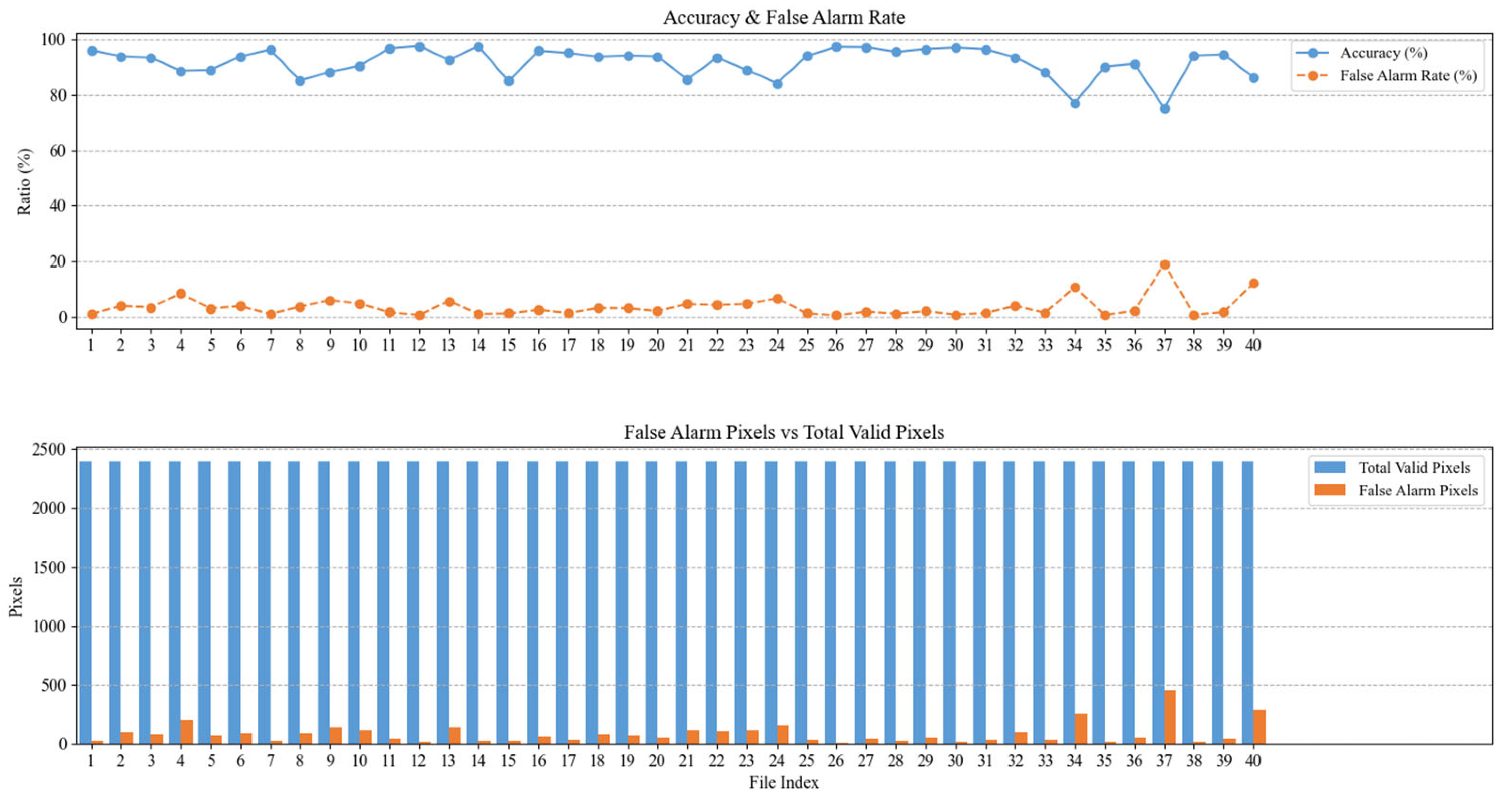
The validation results (Figure 6) indicate that the constructed U-Net model achieved good performance in reproducing remote-sensing-defined bloom patterns, with an overall accuracy of 0.95 and an F1 score of 0.88 for the bloom class. Accordingly, the reported OA and F1 should be interpreted as measures of agreement with remote-sensing-derived labels, rather than direct indicators of ecological prediction skill for cyanobacterial biomass, abundance, or species composition. This suggests that the model not only possessed strong overall discrimination capability, but was also able to identify cyanobacterial bloom targets with relatively stable performance. The fact that the overall accuracy was higher than the F1 score is mainly attributable to class imbalance, as water pixels far outnumbered bloom pixels. Examination of the individual validation samples further shows that most samples maintained a relatively high level of accuracy and a generally low false-positive rate, indicating that the model had good capability for extracting the spatial distribution characteristics of cyanobacterial blooms in Lake Taihu and exhibited a certain degree of generalization ability. Moreover, the errors were concentrated mainly along local boundaries and scattered patches, rather than arising from systematic distortion of the overall spatial structure. The stable convergence observed during model training also indicates that the current input variables, network architecture, and parameter settings were generally effective. At the same time, however, model errors were still influenced by factors such as the spatiotemporal heterogeneity of bloom dynamics, boundary ambiguity, uncertainty in remote sensing labels, the limited number of input variables, and imbalance in sample distribution. In particular, under conditions involving weak blooms, small patches, and complex background features, local misclassification remained likely to occur. Overall, the current model can already provide a relatively reliable basis for cyanobacterial bloom prediction driven by meteorological conditions. Nevertheless, future work should incorporate higher-quality samples, additional water-quality and hydrodynamic variables, and spatiotemporal joint modeling approaches in order to further improve the model’s ability to identify complex scenarios and fine-scale features.

3.3. Impacts of Climate Warming on Cyanobacterial Blooms in Lake Taihu

According to the IPCC Sixth Assessment Report (AR6), the global mean surface temperature has increased by 0.85–0.89 °C over the past century, and climate change is projected to intensify in all regions over the coming decades, with global warming expected to reach or exceed 1.5 °C. The World Climate Research Programme subsequently launched the Coupled Model Intercomparison Project Phase 6 (CMIP6), which represents the most extensive CMIP effort to date in terms of participating models and the most comprehensive in experimental design [28]. The temperature changes under the three scenarios SSP1-2.6, SSP2-4.5, and SSP5-8.5 are summarized below (

Table 1. Warming scenario settings.

Scenario	Air Temperature Setting	Other Variables	Purpose
S0	Baseline value	Kept unchanged	Baseline condition
S1	+1.8 °C	Kept unchanged	Low-warming scenario
S2	+2.7 °C	Kept unchanged	Moderate-warming scenario
S3	+4.4 °C	Kept unchanged	High-warming scenario

) [29,30]:

Based on three representative climate scenarios (SSP1-2.6, SSP2-4.5, and SSP5-8.5), only the air temperature variable was adjusted while all other meteorological conditions were kept unchanged, and the modified inputs were then fed into the trained U-Net model to predict the future spatial distribution and variation characteristics of cyanobacterial blooms in Lake Taihu. By comparing differences in bloom extent, spatial pattern, and magnitude of change under different climate scenarios, the driving effect of rising temperature on the evolution of cyanobacterial blooms in Lake Taihu was analyzed. Thus, the warming scenarios in this study should be interpreted as sensitivity-style temperature perturbation experiments designed to isolate the effect of warming, rather than as fully coupled ecological forecasts in which multiple meteorological and biogeochemical drivers co-vary.

To compare seasonal response intensity, the bloom-area increase under each warming scenario was calculated relative to the baseline condition (S0), and the monthly values were further aggregated by season. Seasonal response strength was then compared using the mean absolute increase in bloom area for spring, summer, autumn, and winter.

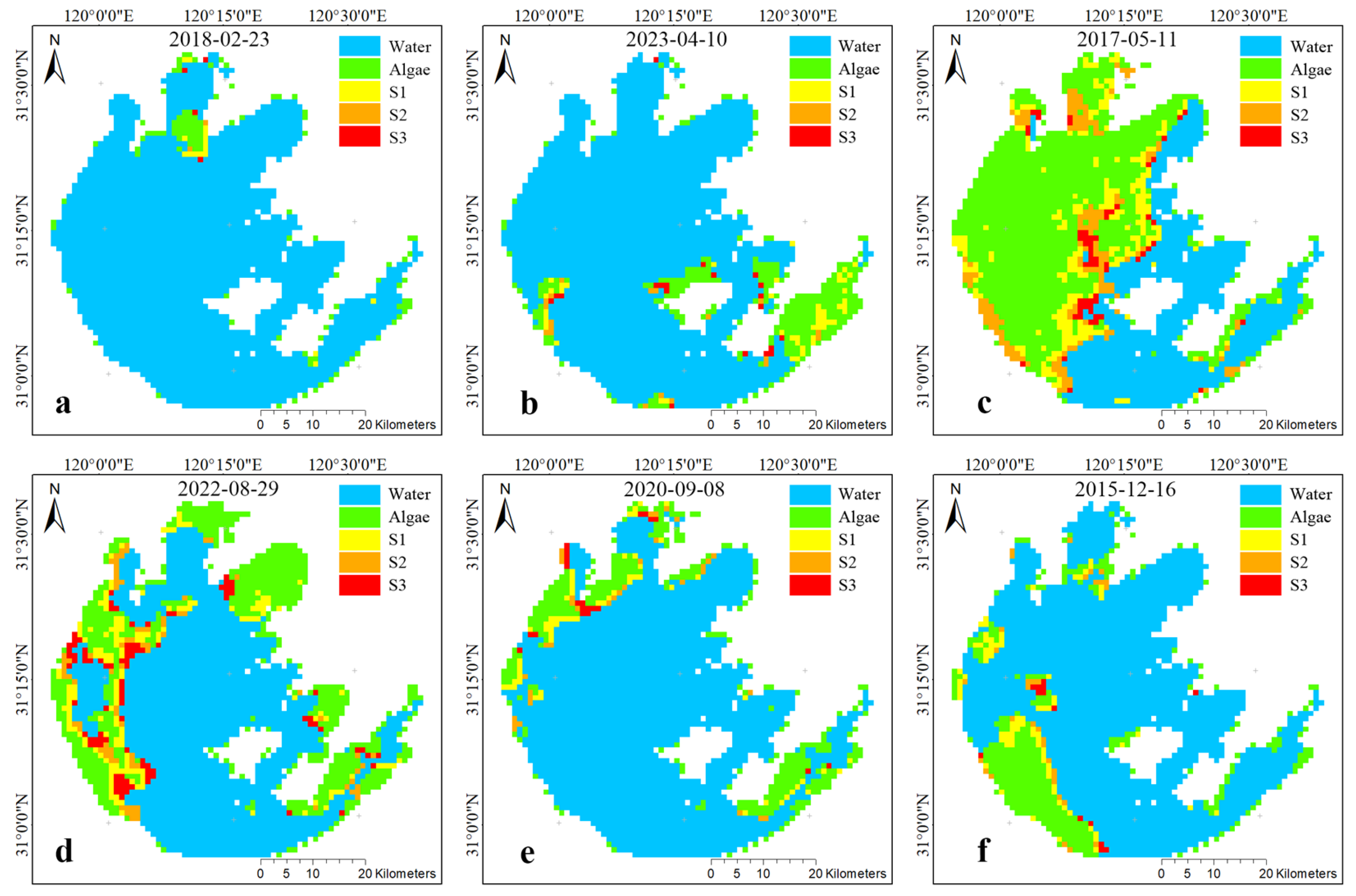
Figure 7 shows that the spatial response of algal blooms to future warming exhibits pronounced seasonal variability and clear stage-dependent characteristics. In late winter and winter (February and December), newly expanded bloom areas were limited and were mainly confined to the margins of existing bloom patches in the northern or southwestern lake regions, with only minor differences among the three warming scenarios. This indicates that under low-temperature background conditions, warming mainly promotes slight outward expansion of pre-existing patches rather than triggering extensive new bloom occurrence, and its effect remains jointly constrained by light availability, hydrodynamic conditions, and initial biomass. In contrast, the warming response became markedly stronger from spring to early autumn (April, May, August, and September), with the highest sensitivity observed in April and May. Newly expanded areas were primarily distributed along the southeastern littoral zone, western shoreline, northern margins, and bay-transition areas, and gradually evolved from scattered patches into more continuous expansion belts as warming intensified, showing combined patterns of edge advancement, patch connectivity, and local infilling. In August and September, the warming effect remained evident, but the newly expanded areas were more concentrated in nearshore zones and bloom-sensitive bay areas, mainly reflected by widening and enhanced continuity of littoral aggregation belts rather than a basin-wide advance toward the lake center. Overall, the spatial response of algal blooms to warming showed a clear seasonal threshold: under low-background conditions, warming mainly caused localized enhancement, whereas during the highly active period from late spring to early autumn, its effect was more fully released and substantially promoted spatial bloom expansion.

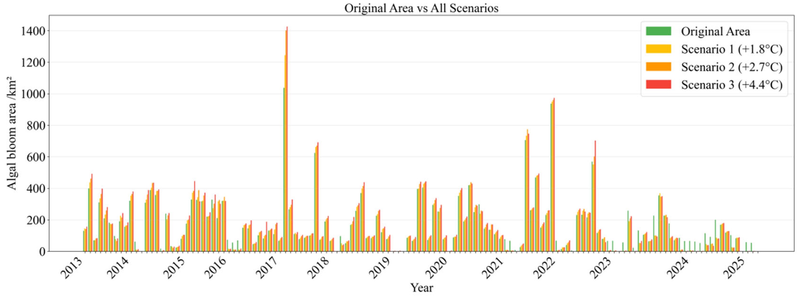
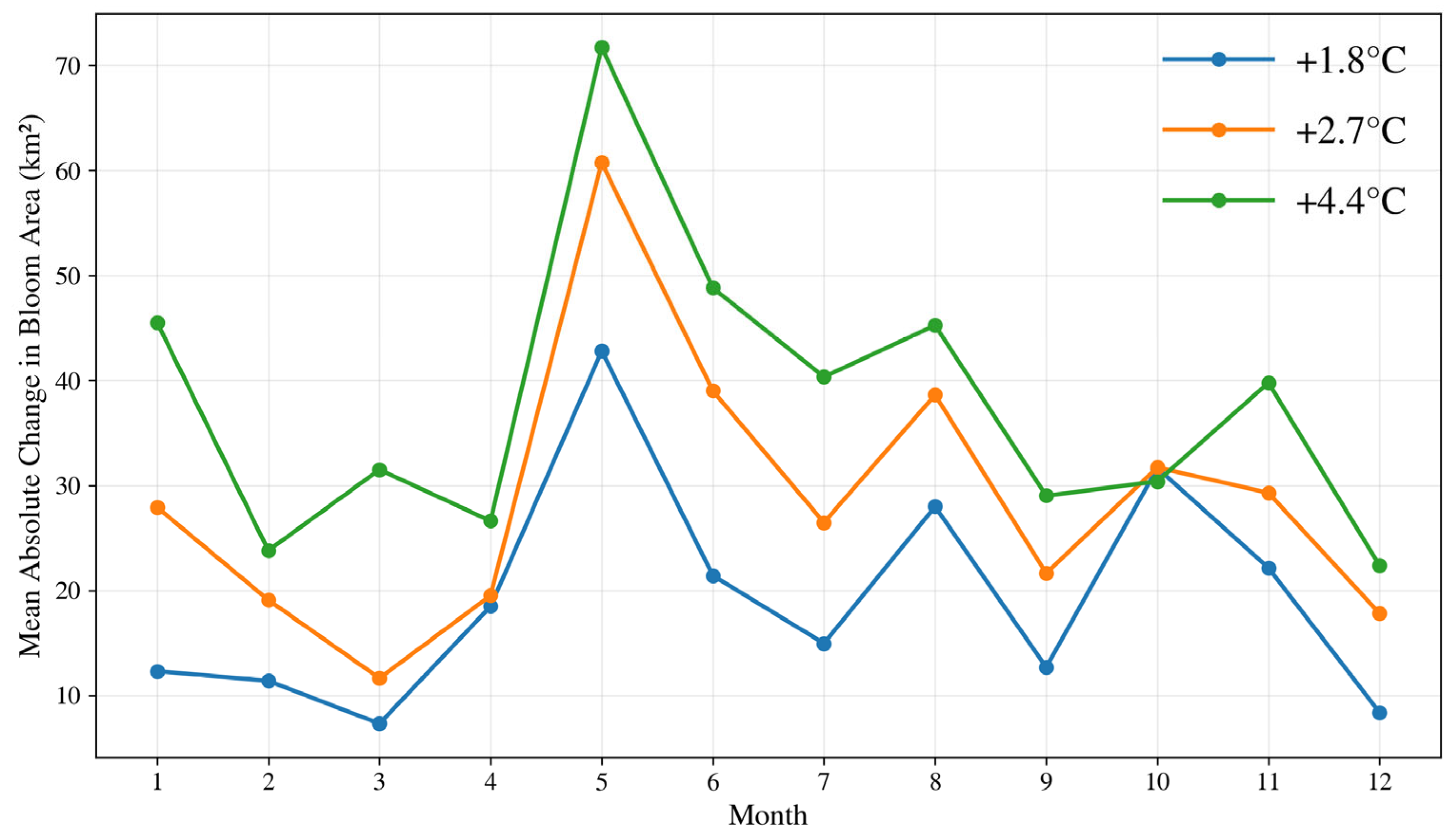
Figure 8 quantitatively confirms the pattern revealed by the spatial distribution maps. Overall, the predicted bloom area under the three warming scenarios was generally larger than the original area and, in most cases, followed an increasing pattern from S1 to S3, indicating an overall positive but not strictly monotonic response to warming. As shown in Figure 9, the annual mean increases were 19.30 km², 28.63 km², and 37.93 km², respectively; compared with the +1.8 °C scenario, the increases under the +2.7 °C and +4.4 °C scenarios were 48.33% and 96.55%, respectively. To compare seasonal response intensity, the bloom-area increase under each warming scenario relative to the baseline condition (S0) was aggregated by season, and seasonal differences were evaluated using the mean absolute increase in bloom area. Based on this comparison, spring exhibited the strongest response, followed by summer and autumn, whereas winter showed the weakest response. At the monthly scale, the peak values for all three scenarios occurred in May, reaching 42.81 km², 60.73 km², and 71.74 km², respectively, indicating that late spring to early summer was the period with the most pronounced warming-related bloom expansion. However, this pattern was not consistent across all samples. In a few cases, bloom area under the higher-warming scenarios showed a slight decline, suggesting that the response of cyanobacterial blooms to temperature increase may be nonlinear and may involve a threshold or an optimal temperature range. Because only three discrete warming increments were examined in this study, the present results do not allow identification of a precise optimum temperature or response threshold.

Combined with Figure 7, when the area differences among warming scenarios were large, the spatial patterns usually corresponded to pronounced outward expansion and enhanced spatial connectivity of newly developed bloom patches; when the area differences were small, the spatial response was more commonly characterized by local edge thickening. This indicates a strong consistency between the area statistics and the spatial configuration. Furthermore, the warming effect exhibited clear background dependence: when the original bloom area was relatively large, the differences among the three scenarios were usually more pronounced, and the peak bloom area under higher warming scenarios was further amplified. In contrast, during periods with relatively low original bloom area, warming still led to an increase in bloom extent, but the overall magnitude of increase was comparatively limited. The few cases in which the predicted bloom area was lower than the initial area mainly occurred during periods with small and highly fragmented bloom patches. This is more likely to reflect the model’s limited ability to identify small-scale and fragmented bloom features, rather than invalidating the overall conclusion that warming promotes bloom expansion.

4. Discussion

The results indicate that the differences between FAI and TCap in cyanobacterial bloom extraction from Lake Taihu essentially reflect the interaction between bloom signal intensity and background interference. Under clear-sky conditions and during periods of intense bloom occurrence, the bloom signal is relatively strong, and the two methods produce largely consistent results. In contrast, during low-bloom periods or under conditions involving thin-cloud interference or complex nearshore backgrounds, mixed pixels and highly reflective backgrounds tend to amplify the differences between the two approaches. FAI is more sensitive to bloom signals, but is also more susceptible to background noise. By integrating information from multiple spectral bands, TCap exhibits greater robustness under complex conditions. This suggests that there is no universally optimal method for remote sensing identification of cyanobacterial blooms; rather, an appropriate balance must be struck between sensitivity and stability.

Further, the meteorology-driven U-Net model was able to reconstruct the overall spatial pattern of blooms reasonably well, indicating that bloom distribution is not random, but instead exhibits relatively stable spatial response relationships with external environmental factors such as air temperature, wind speed, and radiation. However, the model showed weaker performance in predicting small-area and fragmented blooms, suggesting that meteorological factors are more suitable for characterizing bloom patterns at the regional scale, while their explanatory power for local details and short-term aggregation–dispersion processes remains limited. Thus, the present model is more appropriately interpreted as a remote-sensing-based spatial prediction framework than as a fully independent ecological prediction model.

Under warming scenarios, the overall bloom area increased, yet the major bloom centers did not shift substantially; instead, the dominant response was marginal expansion and enhanced connectivity within pre-existing sensitive areas. This suggests that rising temperature acts more as an amplifier of the existing high-risk pattern than as a driver of fundamental spatial reorganization. The stronger response observed in spring further indicates that the effect of warming is strongly season-dependent and is more readily amplified during the transition from low bloom activity to rapid growth. These findings suggest that warming acts as a general promoting factor within the tested temperature increments, but the bloom response is unlikely to be purely linear. Since this study considered only three discrete warming scenarios while keeping other meteorological variables unchanged, the existence of a precise optimum temperature or response threshold could not be resolved and should be further examined using continuous temperature gradients and coupled environmental drivers. Therefore, the findings of this study do not simply demonstrate that “warming increases blooms”; rather, they reveal that, under existing ecological and environmental constraints, climate warming further elevates the risk of cyanobacterial blooms in Lake Taihu by intensifying the expansion of sensitive areas and amplifying seasonal differences.

Several limitations should also be acknowledged. First, the bloom extent analyzed in this study was derived from remote-sensing proxies and was not independently validated against synchronous in situ chlorophyll-a, phycocyanin, or cyanobacterial cell-count measurements for the full study period. Second, the comparison between FAI and TCap was based on visually interpreted reference imagery and should therefore be regarded as a relative image-based benchmark rather than as an independent ecological validation. Third, the U-Net model was trained on remote-sensing-derived binary bloom labels, meaning that its reported performance primarily reflects agreement with remote-sensing-defined bloom patterns. Finally, the warming scenarios were implemented as temperature-only perturbation experiments, with other variables held constant, which helps isolate the effect of warming but does not fully capture the ecological realism of future climate–ecosystem change. Future work should integrate field observations, nutrient dynamics, hydrodynamic processes, and co-varying climate drivers to improve ecological realism and validation strength.

5. Conclusions

This study focused on cyanobacterial blooms in Lake Taihu and systematically investigated remote sensing-based bloom extraction, spatial matching between meteorological variables and bloom data, deep learning-based prediction model development, and bloom responses under warming scenarios. The main conclusions are as follows:

(1)

Both FAI and TCap were effective for cyanobacterial bloom extraction, but their advantages differed. FAI was more sensitive to bloom variation and suitable for rapid identification during high-bloom periods, whereas TCap was more robust under thin-cloud interference and complex background conditions. Their combined use improved the reliability of bloom detection.

(2)

After achieving spatial consistency between meteorological variables and bloom data, the meteorology-driven U-Net model effectively reproduced the spatial distribution and areal variation in cyanobacterial blooms in Lake Taihu, with an overall accuracy of 0.95 and an F1 score of 0.88. The model performed well for medium- and large-area bloom events, demonstrating good applicability for spatial bloom prediction.

(3)

Under the three warming scenarios, bloom area generally increased and spatial expansion became more evident, although the response was not strictly monotonic in all cases. Warming mainly enhanced the outward expansion and connectivity of pre-existing bloom-prone areas rather than shifting the major hotspot locations. Seasonal comparison further showed that the warming response was strongest in spring, followed by summer and autumn, and weakest in winter.

References

1. Huisman, J.; Codd, G.A.; Paerl, H.W.; Ibelings, B.W.; Verspagen, J.M.; Visser, P.M. Cyanobacterial blooms. Nat. Rev. Microbiol. 2018, 16, 471–483. [Google Scholar] [CrossRef] [PubMed]
2. Carmichael, W.W.; Azevedo, S.M.F.O.; An, J.S.; Molica, R.J.R.; Jochimsen, E.M.; Lau, S.; Rinehart, K.L.; Shaw, G.R.; Eaglesham, G.K. Human fatalities from cyanobacteria: Chemical and biological evidence for cyanotoxins. Environ. Health Perspect. 2001, 109, 663–668. [Google Scholar] [CrossRef]
3. Chorus, I.; Welker, M. (Eds.) Toxic Cyanobacteria in Water: A Guide to Their Public Health Consequences, Monitoring and Management, 2nd ed.; CRC Press: Boca Raton, FL, USA, 2021. [Google Scholar]
4. Moustaka-Gouni, M.; Sommer, U. Effects of harmful blooms of large-sized and colonial cyanobacteria on aquatic food webs. Water 2020, 12, 1587. [Google Scholar] [CrossRef]
5. Ayele, H.S.; Atlabachew, M. Review of characterization, factors, impacts, and solutions of Lake eutrophication: Lesson for lake Tana, Ethiopia. Environ. Sci. Pollut. Res. 2021, 28, 14233–14252. [Google Scholar] [CrossRef]
6. Dubey, D.; Dutta, V. Nutrient enrichment in lake ecosystem and its effects on algae and macrophytes. In Environmental Concerns and Sustainable Development; Springer: Singapore, 2019; Volume 2, pp. 81–126. [Google Scholar]
7. Zhang, Y.; Shi, K.; Zhang, Y.; Sun, X.; Li, N.; Huang, X.; Wang, W.; Zhou, Y.; Gao, Y.; Cai, H. The proposal, practice and preliminary application of land-based (ground-based, shore-based) remote sensing of water environment. J. Remote Sens. 2021, 25, 2163–2172. [Google Scholar]
8. Zheng, Y.; Zheng, Y.; Feng, L.; Zhang, C.L.; Li, H.L.; Wang, J.J. Spatially and Temporally Resolved Coastal Ecological and Environmental Observation System for AI Enhanced Harmful Algal Bloom Forecasting. Bull. Natl. Nat. Sci. Found. China 2024, 38, 969–983. [Google Scholar]
9. Zhou, H.W.; Ning, S.; Li, D.; Pan, X.S.; Li, Q.; Zhao, M.; Tang, X. A Sentinel-2 green tide information extraction method incorporating multi-band ratio method and Random Forest algorithm. Chin. J. Mar. Environ. 2024, 43, 119–129. [Google Scholar]
10. Kuang, R.Y.; Zhuang, X.Y.; Xie, S.Y. Spatio-temporal changes of vegetation NDVI in Poyang Lake based on MODIS time series data. Limnology 2026, 27, 143–157. [Google Scholar] [CrossRef]
11. Wang, S.M.; Qin, B.Q. Application of optical remote sensing in harmful algal blooms in lakes: A review. Remote Sens. 2025, 17, 1381. [Google Scholar] [CrossRef]
12. Ou, Z.; Li, X.; Jin, F.; Peng, S.; Liu, W.; Li, E.; Zhang, L. MABI: A novel Mixed Algal Blooms Index based on color space transformation. Mar. Pollut. Bull. 2025, 210, 117321. [Google Scholar] [CrossRef] [PubMed]
13. Colkesen, I.; Ozturk, M.Y.; Altuntas, O.Y. Comparative evaluation of performances of algae indices, pixel-and object-based machine learning algorithms in mapping floating algal blooms using Sentinel-2 imagery. Stoch. Environ. Res. Risk Assess. 2024, 38, 1613–1634. [Google Scholar] [CrossRef]
14. Zhu, Z.; Woodcock, C.E. Object-based cloud and cloud shadow detection in Landsat imagery. Remote Sens. Environ. 2012, 118, 83–94. [Google Scholar] [CrossRef]
15. Louis, J.; Pflug, B.; Debaecker, V.; Mueller-Wilm, U.; Iannone, R.Q.; Boccia, V.; Gascon, F. Evolutions of Sentinel-2 Level-2A cloud masking algorithm Sen2Cor prototype first results. In 2021 IEEE International Geoscience and Remote Sensing Symposium IGARSS; IEEE: New York, NY, USA, 2021; pp. 3041–3044. [Google Scholar]
16. Li, J.; Wu, Z.; Hu, Z.; Jian, C.; Luo, S.; Mou, L.; Zhu, X.X.; Molinier, M. A lightweight deep learning-based cloud detection method for Sentinel-2A imagery fusing multiscale spectral and spatial features. IEEE Trans. Geosci. Remote Sens. 2021, 60, 5401219. [Google Scholar] [CrossRef]
17. Zhang, C.Y. Research on Cloud Detection and Removal Methods for Optical Remote Sensing Images Based on Deep Learning. Master’s Thesis, Jilin University, Changchun, China, 2023. [Google Scholar]
18. Wen, J.F.; Zhang, H.; He, C.X.; Xu, G. Improving Cloud/Snow Detection in Remote Sensing Image with Spatiotemporal Information Fusion. Secur. Commun. Netw. 2022, 2022, 9226401. [Google Scholar] [CrossRef]
19. Yang, Z.X.; Li, Y.X.; Zhu, G.W.; Kang, L.J.; Li, N.; Zhang, Y.L.; Qin, B.Q. Control factors of cyanobacterial bloom area in Lake Taihu, China (2003–2023). J. Lake Sci. 2025, 37, 734–751. [Google Scholar]
20. Chen, N.; Wang, S.; Zhang, X.; Yang, S. A risk assessment method for remote sensing of cyanobacterial blooms in inland waters. Sci. Total Environ. 2020, 740, 140012. [Google Scholar] [CrossRef] [PubMed]
21. Cao, H.Y.; Han, L.; Li, L.Z. A deep learning method for cyanobacterial harmful algae blooms prediction in Taihu Lake, China. Harmful Algae 2022, 113, 102189. [Google Scholar] [CrossRef]
22. Li, J.; Liu, Y.; Xie, S.; Li, M.; Chen, L.; Wu, C.; Yan, D.; Luan, Z. Landsat-satellite-based analysis of long-term temporal spatial dynamics of cyanobacterial blooms: A case study in Taihu Lake. Land 2022, 11, 2197. [Google Scholar] [CrossRef]
23. Hu, C.; Lee, Z.; Ma, R.; Yu, K.; Li, D.; Shang, S. Moderate resolution imaging spectroradiometer (MODIS) observations of cyanobacteria blooms in Taihu Lake, China. J. Geophys. Res. Oceans 2010, 115, C04002. [Google Scholar] [CrossRef]
24. Qi, Q.P. Spatial feature extraction method for surveying and mapping geographic information based on K-T transformation. Surv. World 2022, 5, 42–45. [Google Scholar]
25. Lo, K.S.; Tao, F.L. Method for wetland type extraction using remote sensing combing object-oriented and tasseled cap transformation. Trans. Chin. Soc. Agric. Eng. 2017, 33, 198–203. [Google Scholar]
26. Liang, Z.H. Research on the Construction of Tasseled Cap Transform Indices Time Series Data Sets Based on Spatial-Temporal Fusion Algorithm. Master’s Thesis, Lanzhou University, Lanzhou, China, 2015. [Google Scholar]
27. Ronneberger, O.; Fischer, P.; Brox, T. U-net: Convolutional networks for biomedical image segmentation. In Medical Image Computing and Computer-Assisted Intervention—MICCAI 2015; Springer: Cham, Switzerland, 2015; pp. 234–241. [Google Scholar]
28. O’Neill, B.C.; Tebaldi, C.; van Vuuren, D.P.; Eyring, V.; Friedlingstein, P.; Hurtt, G.; Knutti, R.; Kriegler, E.; Lamarque, J.-F.; Lowe, J.; et al. The scenario model intercomparison project (ScenarioMIP) for CMIP6. Geosci. Model Dev. 2016, 9, 3461–3482. [Google Scholar] [CrossRef]
29. Masson-Delmotte, V.; Zhai, P.M.; Pirani, A.; Conners, S.L.; Péan, C.; Berger, S.; Caud, N.; Chen, Y.; Goldfarb, L.; Gomis, M.I.; et al. Summary for policymakers. In Climate Change 2021: The Physical Science Basis. Contribution of Working Group I to the Sixth Assessment Report of the Intergovernmental Panel on Climate Change; Cambridge University Press: Cambridge, UK, 2023; pp. 3–32. [Google Scholar]
30. Song, F.; Cheng, Y.; Chen, L.; Zhou, K.; Fang, J.; Zhang, M.; Ning, S. Research on Future Precipitation and Runoff Trends in the Ganjiang River Basin Based on CMIP6 Models. Geol. Bull. China 2025, 1–18. [Google Scholar]
Figure 1. Location map of the study area.
Water 18 01065 g001
Figure 2. Spring cyanobacterial bloom distribution (In the first and second columns, green indicates algal blooms. In the third column, bright green indicates algal blooms, while the other colors indicate the lake. In the fourth column, green indicates algal blooms, and blue indicates the lake).
Water 18 01065 g002
Figure 3. Spatial distribution of cyanobacterial blooms in Lake Taihu under cloudy conditions (In the first and second columns, green indicates algal blooms identified by the two methods. In the third column, bright green indicates algal blooms, and white indicates clouds. In the fourth column, bright yellow indicates algal blooms, while some yellow areas indicate clouds).
Water 18 01065 g003
Figure 4. Comparison of relative errors between FAI and TCap under different conditions ((a) Consistency map of algal bloom extraction by the two methods under clear-sky conditions from April to September; (b) clear-sky conditions from October to March; (c) cloudy conditions from April to September; (d) cloudy conditions from October to March).
Water 18 01065 g004
Figure 5. Spatial distribution comparison for the validation set ((af) represent the original data, while the corresponding (a1f1) represent the model prediction results for the corresponding days).
Water 18 01065 g005aWater 18 01065 g005b
Figure 6. Model accuracy on the validation set.
Water 18 01065 g006
Figure 7. Spatial variation under the three warming scenarios ((a) Expanded spatial distribution of algal blooms under three warming scenarios based on the algal bloom distribution on 23 February 2018; (b) corresponding results based on 10 April 2023; (c) corresponding results based on 11 May 2017; (d) corresponding results based on 29 August 2022; (e) corresponding results based on 8 September 2020; (f) corresponding results based on 16 December 2015).
Water 18 01065 g007
Figure 8. Comparison of Bloom Area Changes under Three Warming Scenarios.
Water 18 01065 g008
Figure 9. Monthly mean absolute change in bloom area under three warming scenarios.
Water 18 01065 g009