Article

Identifying Water Stress Hotspots in Chilean Patagonia Using Spatially Explicit Water Yield Modeling and Anthropization Proxies


by
Inigo Irarrazaval
*,
Ángela Hernández-Moreno
,
Paulo Moreno-Meynard
,
Brian L. Reid
and
Cristián Frêne
Centro de Investigación en Ecosistemas de la Patagonia, Coyhaique 5951601, Chile
*
Author to whom correspondence should be addressed.
Water 2026, 18(9), 1041; https://doi.org/10.3390/w18091041
Submission received: 2 March 2026 / Revised: 11 April 2026 / Accepted: 15 April 2026 / Published: 28 April 2026
(This article belongs to the Section Water Resources Management, Policy and Governance)

Abstract

Despite the widespread perception of Chilean Patagonia as water-abundant, the region exhibits marked climatic and landscape heterogeneity. This study evaluates relative water availability across Coyhaique Province (12,712 km2), where projections indicate a trend toward warmer and drier conditions. The province has a marked west–east gradient: humid valleys in the west contrast with much drier areas to the east, where most of the population and development are concentrated. To identify water stress hotspots, we combine spatially explicit water yield estimates derived from the InVEST Seasonal Water Yield model with an anthropization index used as a proxy for water demand, constructing a relative Water Stress Index. The results indicate that water stress increases toward the east, driven by the combined influence of climate variables and anthropogenic pressure. These results indicate that the characterization of Patagonia as uniformly water-rich does not hold at the provincial scale, and highlight the limitations of coarse regional assessments in capturing intra-regional hydrological heterogeneity. The spatial pattern of water stress revealed here exposes a mismatch between the resolution at which hydrological heterogeneity operates and the scale at which prevailing water governance frameworks are formulated, underscoring the need for bottom-up, fine-resolution diagnostics that incorporate local hydrological variability into water planning and governance. The province-scale analysis presented here provides a representative case study for Aysén and illustrates the broader relevance of spatially explicit diagnostics in contexts where regional indicators mask local water stress. Strengthening monitoring networks, protecting headwater catchments, and promoting a decentralized approach to water management remain essential to reduce the risk of human-driven water scarcity.

1. Introduction

Hydrological systems vary spatially across landscapes depending on climatic conditions, topography, and land cover, and are further influenced by anthropogenic pressures [1]. In this context, water stress, defined as the condition in which freshwater supply is insufficient to meet combined human and ecological demand, becomes particularly relevant [2,3]. Such imbalances may lead to competition among uses, ecosystem degradation, or local scarcity. Evaluating water resources in relation to anthropogenic land use is therefore central to sustainable development, as reflected in United Nations Sustainable Development Goal 6.4, which calls for ensuring water availability and sustainable management for all. Because water availability and demand vary markedly across space and time, coarse national or regional indicators often mask critical intra-regional heterogeneity. Landscape-scale analyses are particularly relevant where planning and decision-making occur at the level of sub-basins, provinces, or catchments rather than national aggregates [4]. Spatially explicit, fine-resolution assessments thus provide essential information for decision makers seeking to align water governance with local hydrological realities under increasing climatic and socio-economic pressures.
Climate change future scenarios project an increase in global drought extremes [5]. South American ecosystems in particular have experienced unprecedented droughts in recent years [6]. Chile is no exception to this trend. Since 2010, the center–south of Chile has experienced an unprecedented drought [7], which has impacted rural communities [8], forest ecosystems and wildfires [9,10], and productive activities which depend on water availability [11]. Natural climatic cycles such as El Niño–Southern Oscillation impact water availability [12], and land use change can impact watershed hydrological response and water quality [13,14,15,16,17,18]. Moreover, expected population growth and industrial development can be linked to higher water demand, increasing the stress on water resources [19].
Under projected climate change, water availability is increasingly altered even in regions traditionally considered water-abundant, highlighting the need for reassessing water resources at finer spatial scales to capture local heterogeneity and emerging vulnerabilities [5,20,21]. This is the case of the Chilean Patagonia, which is referred to as a region with plentiful water resources [22,23]. From the Pacific Ocean, there is a sharp west–east decreasing precipitation gradient modulated by the Andes Cordillera. On the Pacific coast, precipitation can exceed 4000 mm yr−1, but 150 km east near the Chilean–Argentinian boundary, precipitation decreases to 300 mm yr−1 or lower [24]. This heterogeneity is frequently overlooked when Chilean Patagonia is treated as a hydrologically homogeneous unit. One example is the Chilean-National Water Balance [25], which is one of the main sources and was updated for reference catchments along Chile in 2017. Water Balance 1987 identified Aysén Region (Región de Aysén) as a water-abundant region and is cited as such in scientific and public policy reports [22,23]. In addition, vastly promoted official state sources, whose objective is to inform decision makers such as local government and municipalities and public services of hydric stress, do not include areas of Patagonia (e.g., Climate Change Risk Atlas for Chile, https://arclim.mma.gob.cl/, accessed 23 October 2025).
This study reassesses the prevailing characterization of uniform water abundance in Chilean Patagonia, focusing on an administrative province: Coyhaique Province, from Aysén Region. Coyhaique Province is located at the leeward side of the Andes Cordillera and is the most populated province of Aysén Region. Here, climate change trends indicate a shift towards a drier and hotter climate [24]. Consequently, accounting for water yield is crucial to provide knowledge on the actual hydric state of the province and support decision makers in adapting to climate change and potential anthropogenic drought [1].
This study contributes a spatially explicit water stress assessment for a data-scarce Patagonian province by integrating InVEST Seasonal Water Yield (InVEST-SWY [26]) with an anthropization-based demand proxy, producing a fine-resolution screening tool capable of identifying relative water stress hotspots that are systematically obscured by coarse regional indicators.
The objectives of this study are: (1) To model the water yield at the landscape scale using a spatially explicit hydrological approach (InVEST-SWY). (2) To build a relative water stress index (WSI) to map spatial patterns of water stress across the province.
To identify areas with critical water supply in relation to water demand, we build upon the widely used concept of water stress index [21,27]. Rather than operationalizing water stress as a supply-to-demand ratio, we construct a spatially explicit relative index that captures the spatial correspondence between water yield and anthropogenic pressure across the landscape. Water stress indices have been applied over multiple spatial scales, from global basins to sub-national units, but their utility increases when implemented at fine spatial resolution, where landscape heterogeneity and diverse water uses are significant [28]. Here, we chose to build a spatially explicit water stress index to ensure that the spatial scale is coherent with the heterogeneity of the landscape and diversity of water uses. The index combines two components: (1) a relative water yield spatial index derived from the InVEST-SWY model, interpreted as a proxy of water supply; and (2) an anthropization index used as a proxy for water demand, reflecting the degree of human land use intensity across the province.
To assess water supply, numerous hydrological models are available, each with distinct advantages and limitations. For example, widely used hydrological models such as SWAT (Soil and Water Assessment Tool [29]), WEAP (Water Evaluation and Planning System [30]), and VIC (Variable Infiltration Capacity [31]) offer process-based or integrated basin-scale simulations of water flow, storage, and allocation. On the other hand, models such as InVEST-SWY [26] provide a spatially explicit approach, have relatively low data input requirements, and are particularly used to inform decision makers about water availability, watershed prioritization, and ecosystem service trade-offs at local to regional scales [32,33,34,35]. Given these characteristics and considering the scarce hydrological data available in Patagonia [36,37] and our focus on supporting policymaking, we selected the InVEST-SWY model as the most suitable framework for our assessment.
In Coyhaique Province, water demand is difficult to quantify because many rural areas depend on unmonitored streams and wells. To address this limitation, we use the anthropization index [38] as a proxy for demand and combine it with water availability to develop a water stress index. Anthropization, understood as the transformation of natural landscapes through human activities, has been widely recognized as a key driver of changes in ecosystem structure and functioning, including the water cycle [39,40,41]. To quantify this influence, a range of spatially explicit indicators based on land use and land cover (LULC) has been developed, including widely used frameworks such as the Human Footprint [42,43], which integrates multiple pressures (e.g., infrastructure, population density, and land transformation) to map cumulative human impact on ecosystems [43], as well as related indices capturing human pressure gradients, such as hemeroby [44], naturalness [45], or land use intensity across spatial scales [38]. Following this approach, we use an anthropization index derived from LULC data [38,46] as a proxy for potential water demand. This index captures the spatial intensity of human activities, such as urban expansion, agriculture, and other forms of intensive land use, that influence hydrological processes. Although it does not directly quantify water withdrawals, it provides a spatially consistent representation of anthropogenic pressure, enabling the identification of areas where potential demand may interact with limited water availability, particularly in data-scarce regions. This allows us to identify relative critical areas of vulnerability to limited water resources and to discuss policy strategies and territorial planning guidelines aimed at reducing the risk of human-driven water scarcity.

2. Materials and Methods

2.1. Study Area

Coyhaique Province (45.5° S–72.0° W; Figure 1) lies within the administrative Aysén Region (Región de Aysén), part of the Chilean Patagonia (41.5° S–55.5° S). Within the study area, several rural settlements and urban centers are present. Coyhaique, the provincial and regional capital, concentrates the largest population (~60,000 inhabitants) and is located near the central part of the province, within the mesic–dry climatic transition on the leeward side of the Andes. To the north of Coyhaique, rural localities such as Villa Ñirehuao, Villa La Tapera, and Villa Ortega are situated in intermontane valleys. The southeast settlements, including Valle Simpson, El Blanco, and Balmaceda, are aligned along the Simpson Valley and the main transport corridor. In contrast, Puerto Aysén lies to the west, closer to the fjord system.
The Patagonian region is characterized by an extreme west–east precipitation gradient that shapes its hydrological and ecological diversity. Most precipitation is produced by the southern westerlies and orographic uplift over the Andes, exceeding 5000–6000 mm yr−1 on the Pacific slopes and declining to ~300 mm yr−1 on the leeward side within less than 100 km. South of ~42° S, the Andes bisect the Chilean territory, separating coastal archipelagos to the west from the valleys to the east. This configuration amplifies the rain-shadow effect, as moist air masses lose most of their moisture on the windward slopes, leaving eastern Patagonia increasingly dry. At interannual and decadal scales, precipitation variability is influenced by the Southern Annular Mode and El Niño–Southern Oscillation (ENSO), while long-term records indicate a decline in precipitation in the last decades [24]. According to the Köppen–Geiger classification, three main climates coexist within short distances: temperate evergreen forests in the humid west, cold steppe with deciduous vegetation in the east, and alpine tundra in the highlands [47,48].
Unlike latitudes north of 40° S, where precipitation increases eastward across the Andes, the southern transect across Coyhaique Province exhibits the opposite pattern, with mean annual precipitation declining sharply from west to east (Figure 1), a gradient inversion that underscores the relevance of province-scale hydrological diagnostics. Figure 1 compares these gradients across four elevation–precipitation profiles south of 35.5° S of the Andes. While in the northern profiles (a–a′, b–b′, c–c′) precipitation increases eastward, the southern transect (d–d′) across Coyhaique Province shows the opposite pattern, with precipitation declining sharply from west to east. Along this transect, mean annual precipitation reaches ~3000 mm in Puerto Aysén, decreases to ~900 mm in Coyhaique, and drops to ~150 mm in Balmaceda, yielding a provincial mean near 1400 mm yr−1 [49]. For reference, note the 1000 mm yr−1 blue dashed line, which highlights the contrasting trends. Although Coyhaique’s temperate climate differs from central Chile, its annual precipitation is comparable to Mediterranean regions such as Linares Province (~1350 mm yr−1 at 35.5° S). This pronounced rain-shadow effect explains the reduced precipitation observed in Coyhaique’s upstream catchments.

2.2. Water Yield at the Landscape Scale Using InVEST-SWY

2.2.1. Model Description

To model water yield, we applied InVEST-SWY [26], a spatially explicit hydrological model that provides the relative contributions of the water balance components such as direct runoff, base flow, and local recharge on a monthly basis at a pixel scale. The InVEST-SWY model is based on the water balance equation, which states that water inflows equal outflows over a given time period. Inflows correspond to precipitation (P), while outflows include discharge (Q) and evapotranspiration (ET). The differences between inflows and outflows correspond to the variation in water storage (ΔS) for a certain time period. Given the above, the water balance equation is defined as:
ΔS = PETQ
where Δ S , P , E T , and Q are all expressed in [mm], as InVEST-SWY computes all water balance components as water depth accumulated at each cell or pixel over a given time period. These depth values can be converted to volumetric discharge [m3 s−1] by multiplying by cell area and dividing by the time step. InVEST-SWY was selected as described in the introduction, given its spatial explicitness and suitability for a data-scarce context. This is particularly relevant in Patagonia, where sparse meteorological networks, data scarcity, and observational gaps are characteristic of the region [50].
As an overview, the InVEST-SWY workflow includes defining inputs from meteorological variables (precipitation and reference evapotranspiration), land cover (LULC), and digital elevation models to compute water mass balance at each pixel (30 m) and at a monthly time step. Each of the LULC categories is linked to an infiltration and evapotranspiration value (Table 1). Then, the model computes the infiltration process based on the curve number approach [51,52,53] and evapotranspiration based on the crop index [54,55]. Water loss or gain at each pixel is diverted to downstream pixels defined by a flow routing algorithm. Lastly, the model partitions the water input into direct flow (quick flow), basal recharge (base flow), local recharge, and actual evapotranspiration. Quick flow or direct runoff corresponds to the portion of precipitation that runs on the surface (is not infiltrated or evaporated) and contributes to river discharge. Quick flow is associated with water regulation function [32,56]. Base flow corresponds to water that has been infiltrated and contributes to stream discharge. Base flow is associated with the water supply function. Local recharge represents water that infiltrates and has the potential to contribute to base flow and is associated with the water storage function. Local recharge can be negative if a pixel does not receive enough water to satisfy the vegetation requirement and uses water from upstream pixels. A complete description of InVEST-SWY can be found in [26]. InVEST-SWY does not explicitly simulate snowpack accumulation or melt dynamics, treating all precipitation as liquid. However, in Coyhaique Province, snowfall and snowmelt are largely confined within the same year, so the annual water balance is approximately conserved. Accordingly, model performance was evaluated against annually aggregated observed discharge, ensuring modeled and observed values correspond to the same temporal scale. In addition, we evaluate InVEST-SWY outputs as spatially explicit indexes that quantify the relative contribution of a parcel of land or pixel [34].

2.2.2. Data Requirements

Modeling data requirements by InVEST-SWY include hydrological variables, the elevation model, land cover maps, as well as vegetation biophysical parameters. Hydrometeorological data was obtained from datasets from CAMELS-CL [49] for the years 1979–2018 at a monthly time step. The datasets are derived from statistical regionalization of the atmospheric reanalysis ERA-Interim. Then, evapotranspiration was computed using temperature and radiation by applying the Hargreaves–Samani equation [57]. Land use/land cover (LULC) maps for Coyhaique Province were obtained from [46]. These original maps included 20 land cover classes derived from satellite image classification but did not distinguish between deciduous and evergreen forests. Because tree phenology (evergreen vs. deciduous) strongly affects evapotranspiration dynamics, especially in regions with seasonal climate, we refined the forest classes by overlaying the LULC maps with a bioclimatic raster [58]. We aggregated the bioclimatic model into three broad categories: evergreen forest, deciduous forest, and bare soil. Then, for each pixel originally classified as “forest” in the LULC map, we assigned a new class (“evergreen–forest” or “deciduous–forest”) according to the underlying bioclimatic classification. As a result of this reclassification, the final LULC map includes 27 categories.
The digital elevation model was obtained from [59]. Four soil types were obtained from the Global Hydrologic Soil Groups [60]. The classes vary from low runoff to high runoff potential (A, B, C, and D). Soil classes for wet soil and high runoff potential (A/D, B/D, C/D, and D/D) were reclassified as D to meet InVEST-SWY requirements. Biophysical parameters include evaporation crop coefficient [54] and curve number [51,53]. Monthly crop coefficients for each LULC category were derived from normalized-difference-vegetation-index (NDVI) following [55]. First, we obtained NDVI from the MODIS 16-day product (MOD13Q1 and MYD13Q1) at 250 m resolution. Second, we computed average monthly NDVIs. Third, we computed the average NDVI for each LULC category for each month. Lastly, we applied a linear function to transform NDVI indexes into evapotranspiration crop coefficients (kc,j = 1.457 NDVIj −0.1725) [55]. Note that here it is critical to have divided LULC categories into deciduous and non-deciduous, as deciduous NDVI during the winter season is much lower compared to non-deciduous trees. Curve numbers for each LULC category were obtained from [52,61]. Lastly, InVEST-SWY harmonizes all spatial inputs by resampling them to the resolution of the digital elevation model (DEM), which defines the effective spatial resolution of the analysis [26].
Table 1. Input datasets.
DataVariableFormat UnitResolutionSource
Landcover and biophysical properties
LandcoverLULC 2018.Categories 27Raster 30 mDerived from LULC [46] and bioclimatic and vegetational synopsis [58]
Land cover biophysical propertiesSoil typeCategories 4. (A, B, C and D)Raster 250 mGlobal Hydrologic Soil Groups, HYSOGs250m [60]
Curve number (CN)27 categories and for each soil type. Range 0–100-Curve number [52] and this study.
Evapotranspiration correction factor (kc)-Monthly for each 27 landcover classDerived from NDVI (MOD13Q1 and MYD13Q1) for each LULC and linear transformation [55]
Hydro-meteorological data
Hydro-meteorological dataPrecipitationmm1979–2018 monthly.
Raster 5 km
CR2 [49]
Temperature°C1979–2018 monthly.
Raster 5 km,
CR2 [49]
EvapotranspirationmmRaster 5 km, monthlyDerived from temperature [49], and solar radiation [57].
Discharge for 13 watershedsm3 s−11979–2018 time series Monthly/dailyCAMELS basins [49]
Topography
Digital elevation modelDigital elevation modelmRaster 30 mNASA, & JPL [59]
Watershed delineation-PolygonCAMELS basins [49]
Water intakes and catchmentsAPR, APU catchments Polygons[62]

2.2.3. Model Evaluation Against Observed Data

To evaluate the model biases, we compared modeled and observed discharge from years 1979–2018 at thirteen watersheds inside the study area (Coyhaique Province, Figure 2). The watershed delineation and discharge were selected from the CAMELS-CL dataset [49].
First, we ran InVEST-SWY forced with climate data from 1979 to 2018. To evaluate the sensitivity of modeled water yield to land cover representation, the model was run separately for each of the three available LULC maps (1984, 2000, and 2018). The results indicated that the LULC year had a negligible influence on modeled discharge at the watershed scale from CAMELS-CL, with volumetric water yield estimates remaining largely consistent across all three scenarios. This insensitivity is consistent with the relatively stable landscape documented for Coyhaique Province over this period, where fewer than 5% of pixels changed land cover class between 1984 and 2018 [46]. Given this stability and the marginal sensitivity of model outputs to LULC year, the 2018 land cover map was selected for the main results.
Second, we compute watershed discharge for the selected watersheds. As InVEST-SWY provides an estimate of the water balance in mm at each pixel, we follow a similar strategy as in previous studies: we aggregate the model outputs, quick flow and base flow (in mm), on a watershed scale to obtain an annual modeled watershed discharge [32,34,35]. This procedure allows for obtaining a modeled discharge time series (1978–2018), which can be compared to observed discharge, as commonly done in hydrology [63].
Lastly, we assess the mismatch of modeled versus observed discharge from 1979 to 2018 at the thirteen selected watersheds. We use the Pearson correlation index and bias statistics to evaluate model performance. It is important to notice that InVEST-SWY recommends following a relatively observation/modeled assessment [34]. Then, the comparison between observed and modeled discharge is done with respect to the relative correlation and not in terms of systematic bias. This procedure allows us to identify the variance of the errors and biases, and the relative discharge between watersheds should be well represented [32,34].

2.3. Water Stress Index

The WSI is constructed by combining modeled water yield from InVEST-SWY with an anthropization index used as a proxy for water demand. To characterize water yield, quick flow and base flow are summed at each pixel and averaged over the period 2014–2018. This five-year window reduces interannual variability, providing more stable estimates. As recommended in the InVEST-SWY guidelines, these outputs are interpreted as relative indexes rather than absolute values [26,34].
To represent water demand, we used the anthropization index of Coyhaique Province [38] as a spatial proxy. We assume that a higher degree of anthropization (e.g., exotic tree plantations, agricultural land, pastures, and urban areas) reflects greater water demand, whereas lower values (e.g., old-growth forests, steppes, and wetlands) indicate lower demand. Notably, agriculture in this region is predominantly rainfed rather than irrigated; thus, the highest water consumption is associated with urban areas. It is important to note that land use transformation and water demand are not independent processes. More intensive land uses, such as exotic tree plantations and improved pasturelands, are associated with greater biomass production per unit time and, consequently, higher evapotranspiration demands relative to native vegetation. These improved pasturelands are typically established through state-subsidized land management programs such as System of Incentives for the Agri-environmental Sustainability of Agricultural Soils [64], which incentivize biomass productivity improvements across agricultural lands in Chile. In this sense, the anthropization index captures not only the spatial extent of land transformation but also its functional implications for water demand. Nevertheless, we acknowledge that this proxy does not disaggregate individual demand sectors and should be interpreted as a relative spatial indicator of anthropogenic pressure on water resources rather than a direct measure of volumetric water consumption (see Section 4.3). Finally, both the water yield index and the anthropization-based demand index were rescaled to a common 0–1 range using min–max scaling:
Xscaled,i = (XiXmin)/(XmaxXmin)
where Xi is the value of the variable in spatial unit i, and Xmin and Xmax are the minimum and maximum values observed across all spatial units in the study area. This procedure was applied separately to the water yield index and the anthropization index.
The water stress index (WSI) was then calculated as:
WSIiraw = Ascaled,iWscaled,i
where Ascaled,i is the scaled anthropization-based demand index, and Wscaled,i is the scaled water yield index for spatial unit i. This formulation is conceptually based on the balance between water demand and water supply: water stress increases where anthropogenic demand is high relative to water yield and decreases where water yield exceeds demand. Lastly, WSIiraw which may range from −1 to 1, is rescaled to 0 to 1 using Equation (2) to obtain the WSI. Under this formulation, values of WSI close to 1 indicate areas with relatively higher water stress, whereas values close to 0 indicate areas with relatively lower water stress. To support the interpretation of spatial discontinuities in water stress, the final WSI values were classified using the Jenks natural breaks method, which is designed to identify inherent groupings and sharp transitions in the data distribution.

3. Results

3.1. Water Yield Model by InVEST-SWY

3.1.1. Water Yield

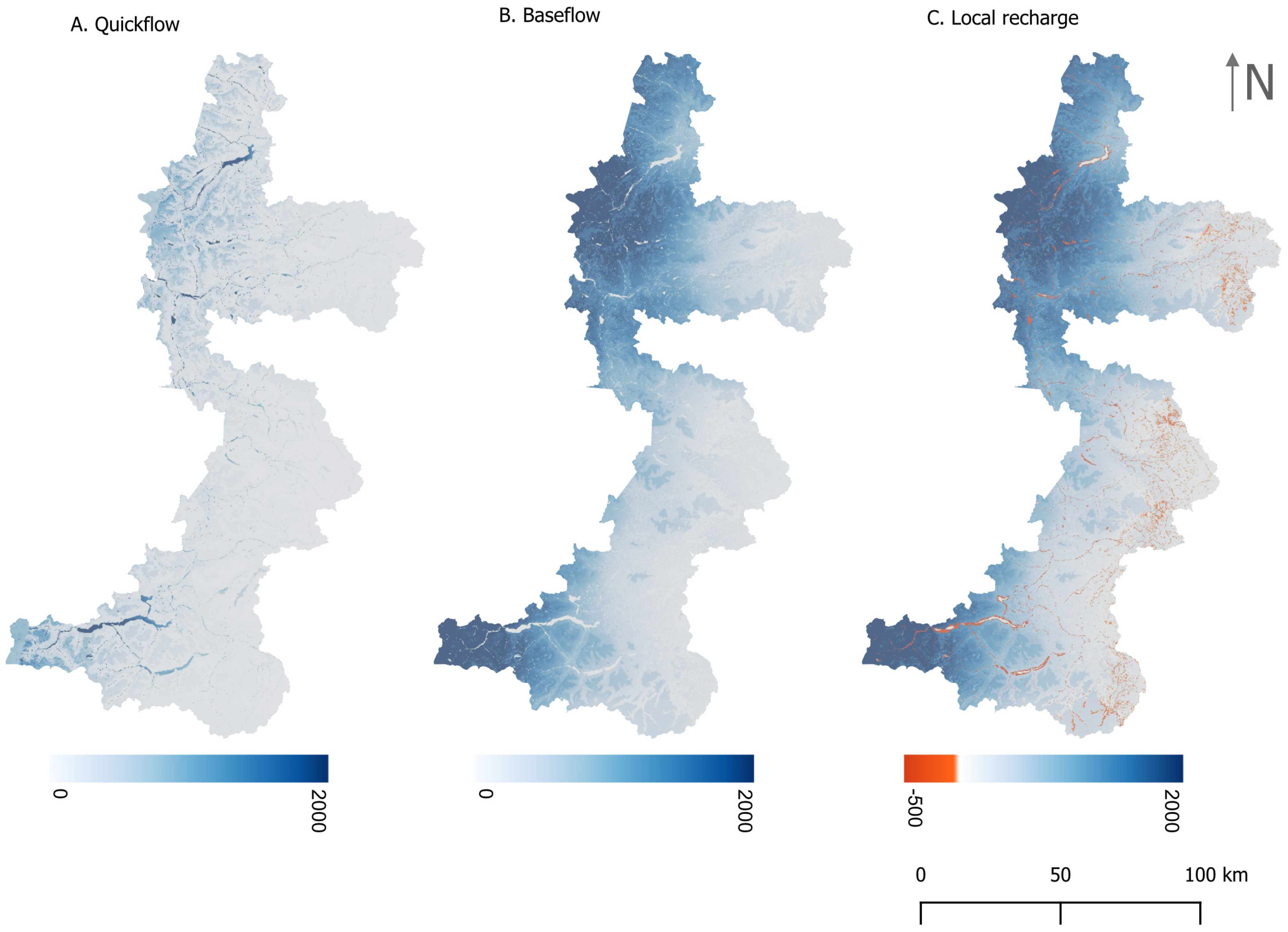
The InVEST-SWY model spatially explicit results are presented, decomposed into quick flow (direct runoff), base flow, and local recharge (Figure 2). At the province scale, it can be observed that water yield follows a general west–east gradient, where the pixels with the highest values are mainly in mountainous areas with high slopes covered by primary forest, while pixels with lower values are mainly distributed in the east of the study area on the Patagonian steppe. The quick flow and base flow spatial models showed values ranging between 0 and 2000 mm. The quick flow corresponded to a fraction of base flow (~13.6%), with the latter being the main contributor to river discharge (Supplementary Materials Figure S2).
The local recharge spatial model added negative values to the scale up to −500 mm distributed mainly to the east of Coyhaique Province (red color pixels, Figure 2C). In InVEST-SWY, local recharge represents the net water available for subsurface flow at the pixel scale, derived from precipitation and actual evapotranspiration. Positive values indicate a local surplus available for infiltration or lateral flow, whereas negative values indicate a local deficit, where evapotranspiration exceeds precipitation and upstream contributions are required to sustain water availability. Here, negative local recharge values produced by the InVEST-SWY occurred in two situations: (1) pixels corresponding to permanent open water bodies and river channels where water evapotranspiration exceeds precipitation, and (2) terrestrial pixels where high evapotranspiration and the absence of lateral inflows yield a local water deficit (requiring upstream pixels to sustain water availability).

3.1.2. Evaluation Against Observed Data

As InVEST-SWY is designed to produce spatially explicit relative indices of water yield rather than volumetric discharge estimates [26,34], model assessment was conducted following the approach of Benra et al. (2021) [32], comparing modeled outputs against observed discharge from thirteen CAMELS-CL catchments across Coyhaique Province. This exercise goes beyond the intended use of InVEST-SWY in many comparable studies, which limit their assessment to the interpretation of spatial indices without comparison against observed data. The results indicate that the model captures the relative spatial distribution of water yield across the province, with nine of thirteen catchments showing significant correlations with observations (r > 0.5). Modeled discharge was consistently underestimated across all catchments, but because this bias is systematic and uniform in direction, relative differences among catchments are preserved, supporting the validity of inter-catchment comparisons. Full performance statistics, including Pearson correlation coefficients, mean bias, and relative bias per catchment, are reported in Supplementary Materials Table S1 and Figure S1.

3.2. Relative Water Stress Index

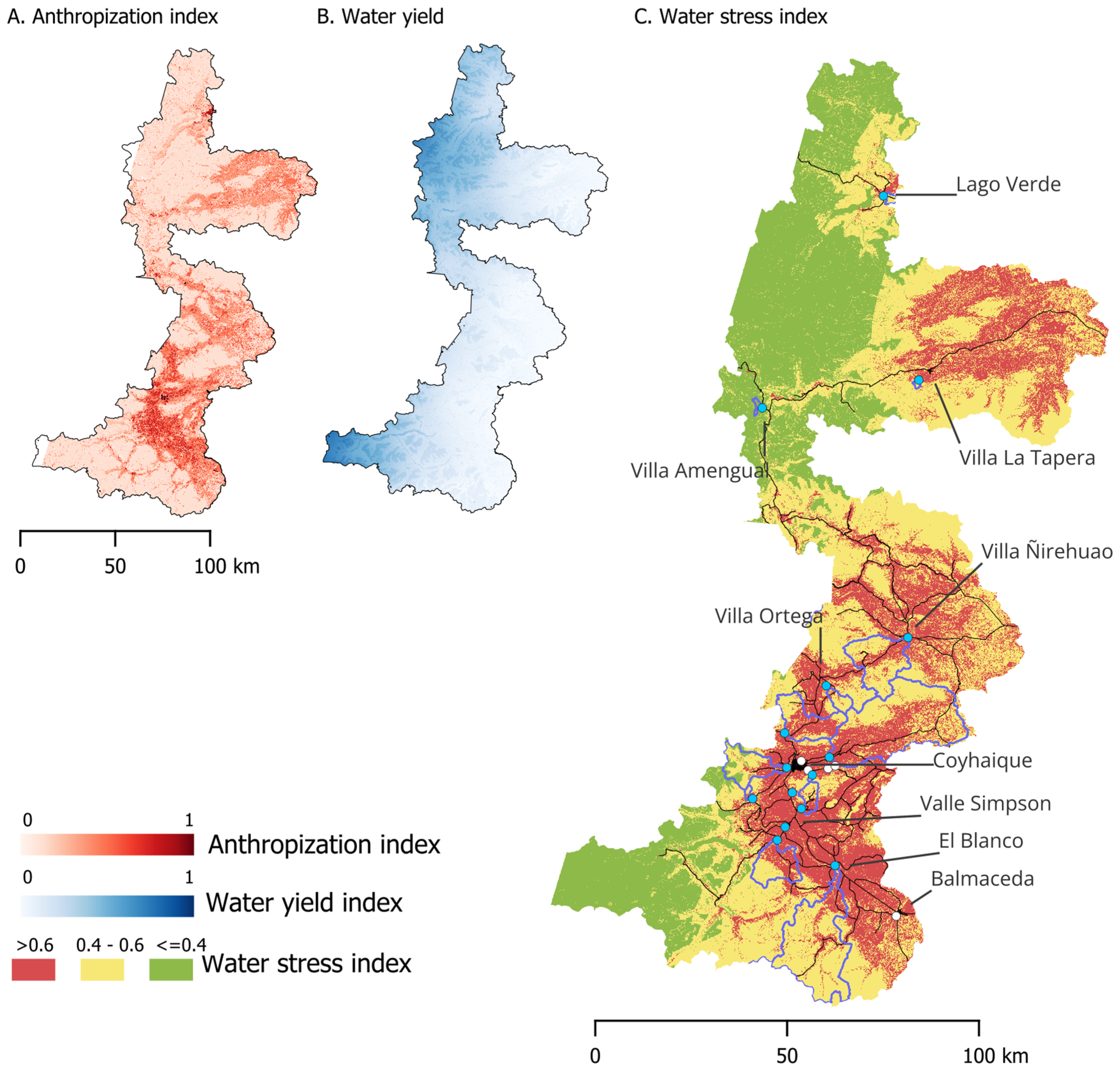
Combining the anthropization index [38] (Figure 3A) along with water yield (Figure 3B), the water stress index is obtained (Figure 3C). To classify the spatial distribution of the water stress index (WSI), we applied the Jenks natural breaks. Based on this approach, WSI values were grouped into three categories: low, medium, and high (Figure 3C). The water stress index reveals a clear pattern of increasing hydric stress toward the eastern part of the province. This gradient reflects the combined influence of climatic factors and land use intensity, where agricultural and urban areas exhibit greater stress. In Table 2, the statistics of the water stress index are presented. High water stress areas cover 3336 km2, medium stress areas 5425 km2, and low stress areas 3787 km2. High-stress zones (WSI > 0.6) exhibit a median WSI of 0.69 (range 0.60–1.00). These areas are characterized by the lowest median water yield index (0.07; range 0.00–0.55) and the highest anthropization index (median 0.50; range 0.25–1.00). In contrast, low-stress areas (WSI ≤ 0.4) show a median WSI of 0.32 (range 0.00–0.41), associated with high median water yield (0.50; range 0.19–1.00) and low anthropization (median 0.13; range 0.00–0.63). Medium-stress areas present intermediate values (median WSI 0.51; water yield median 0.15; anthropization median 0.13).
Spatially, high WSI values concentrate east of Villa La Tapera, in the Villa Ñirehuao area, and in the eastern and southeastern sectors of Coyhaique, including the Simpson watershed with towns of Valle Simpson, El Blanco, and Balmaceda. These sectors combine a structurally low water supply and elevated anthropogenic pressure. Conversely, the western mountainous areas, dominated by forest and lower human intervention, display low WSI values, reflecting high water yield and limited demand.
Overall, the quantitative distribution of WSI classes confirms that water stress in Coyhaique Province is not homogeneous but spatially structured, with approximately one-quarter of the provincial area falling under high relative water stress. These results reinforce the importance of sub-provincial diagnostics to identify localized vulnerabilities within regions commonly perceived as water-abundant.

4. Discussion

4.1. Priority Water Stress Areas

At the provincial scale, three main areas emerge as priority areas for water management: Coyhaique, Valle Simpson, and Villa Ñirehuao (Figure 3C). These areas correspond to the watersheds of Coyhaique, Valle Simpson, and Villa Ñirehuao rivers and are characterized by comparatively low water yield relative to the rest of the province, reflecting both the regional precipitation gradient and local land use pressures.
Figure 3C shows drinking-water intakes (light-blue dots) and their respective catchments (blue polygons). Most rural and urban water supply systems (APR and APU) depend on surface water sources [62], with Valle Simpson being the only exception where groundwater is used.
These systems collectively serve the largest share of Coyhaique Province’s population, with the Coyhaique APU alone supplying more than 60,000 inhabitants through four surface water intakes, three of which fall within watersheds classified as high water stress [62]. Zonal statistics of the WSI across all mapped drinking-water catchments confirm this pattern: the Coyhaique catchments (Coyhaique bajo and Alto Baguales, Supplementary Materials Figure S2) exhibit the highest median WSI values among all drinking-water supply areas (0.57 and 0.61 respectively, Table S2), while the APR near the south Coyhaique catchment also exceeds the high-stress threshold (median WSI 0.58, El Salto in Figure S3). In contrast, the APR located in the western sector presents the lowest median WSI (0.44). Refer to Supplementary Materials Table S2 and Figure S3.
These systems are concentrated in the drier eastern sub-basins, making them more exposed to hydrological variability and potential seasonal shortages. This structural exposure is compounded by the absence of alternative water sources for the vast majority of these systems [62], leaving communities with limited adaptive capacity under drought conditions. The Coyhaique APU system, the largest urban population in Aysén, draws water from sub-basins identified as relatively high-stress. This represents a structural vulnerability: the region’s main urban center depends on catchments with low water yield and increasing land use pressures. Anticipated urban expansion in the upper and middle watersheds, where development potential is greatest, may further compromise water quality and hydrological regulation.
Similar dynamics occur in the Simpson Valley, which follows the main highways toward Balmaceda and concentrates a large part of the region’s productive grasslands, in addition to a high density of buildings. Other studies [65] reported comparable hydrological risks in this area, supporting our assessment and indicating convergent evidence of water stress near Coyhaique’s urban interface.
The Ñirehuao basin represents a transitional zone where climatic and topographic contrasts amplify the sensitivity of surface-water systems, with a median catchment WSI of 0.54 and spatial variability extending to maximum values of 0.874 (Table S2). Rural settlements such as Villa Ñirehuao, Villa Ortega, and Villa Tapera depend on these marginal water sources, reinforcing the need for localized management approaches.
Overall, these results emphasize the need to integrate land use regulation, urban planning, and watershed protection to maintain ecosystem functions of water regulation, supply, and storage in Coyhaique and neighboring basins.

4.2. Public Policies on Land Use, Water Demand, and Water Availability

4.2.1. Spatial Scale Mismatch in Water Management

Results show that Coyhaique Province exhibits marked spatial heterogeneity in water stress, with high-stress hotspots concentrated in the eastern sectors where population density and land use pressure are highest. This pattern reflects a fundamental scale mismatch between hydrological reality and prevailing water governance frameworks in Chile, which are typically formulated at broad administrative or catchment scales with limited consideration of intra-regional heterogeneity. The concept of the southern Andes as “mountain water towers” [20,66] is broadly valid north of 40° S, but does not translate directly to Patagonia, where orographic precipitation declines sharply eastward, generating pronounced spatial variability in water yield within short distances. Coarse regional assessments that treat Aysén as uniformly water-abundant do not capture this gradient, exemplified by national drought tools such as ArClim [67], which begin their analysis north of 40° S, omitting Patagonia altogether. Relying on large administrative or hydrological units risks masking localized deficits: in Coyhaique Province, upstream communities may experience water scarcity even when downstream flow appears abundant. Recent assessments confirm this concern, with nearly one-third of Patagonian basins exhibiting moderate to high water stress despite the region’s overall water surplus [62].
Scale mismatches between governance frameworks and hydrological heterogeneity are not unique to Patagonia, and comparable dynamics have been documented across the European Alps, western United States, and Andean systems, where basin-scale policies frequently obscure sub-catchment water deficits driven by orographic gradients and concentrated demand [20,66,68].
The spatial pattern observed in Coyhaique Province reflects a broader mountain-region dynamic, underscoring the need to align national governance frameworks with spatially explicit, bottom-up strategies that account for intra-regional hydrological contrasts under shifting climatic and socio-economic conditions.

4.2.2. Limits of Stationary Assumptions Under Climate Change

Water use in Chile operates under a system of tradable private water use rights that relies on assumptions of hydrological stationarity [69]. Three interrelated limitations undermine its adequacy under current and projected climatic conditions. First, water rights are granted based on historical mean discharge, using a probability of exceedance greater than 85% to estimate water availability, which does not account for long-term trends in streamflow decline [70]. Second, ecological flow thresholds, defined as 20% of the historical mean or 50% of the 95% exceedance discharge, likely underestimate actual ecosystem requirements [71]. Third, the legal framework does not permit dynamic adjustment of water rights in response to changing hydrological conditions, as rights can only be revoked on administrative grounds.
The Simpson watershed in Coyhaique Province illustrates these structural constraints: annual discharge has declined by 36% relative to its historical mean [65], yet allocations continue to be issued without adjustment. Addressing these gaps requires aligning water rights allocation with updated climate projections, land use change assessments, and ecologically informed flow requirements. Moreover, it should be noted that the present assessment does not capture temporally dynamic demand components such as seasonal domestic peaks, tourism, or industrial uses. Quantifying these disaggregated demand sources remains a priority for future research, contingent on the availability of sector-specific consumption data currently lacking for the province.

4.3. InVEST-SWY Modeling Challenges and Limitations

Estimating the water balance through hydrological models has become a standard approach to understand watershed response to climatic forcing and is useful for policy making [72,73]. InVEST-SWY provides a spatially explicit model of water yield. The choice of InVEST-SWY is particularly suited for this application, given its relatively low input data requirements, and it is spatially explicit and therefore useful for land use policy and management. Note that other water balance models (e.g., SWAT and WEAP) compute water balance at smaller time steps and can provide quantitative information on water yield [74,75]. However, the implementation requires much more comprehensive hydrometeorological datasets. Systematic underestimation of the modeled discharge can be due to the inputs’ uncertainty and evapotranspiration estimates, which were derived from crop coefficients. However, the aim of the study is to analyze the relative spatial patterns rather than water volume quantification. Lastly, to reduce uncertainty from hydrological models, further efforts should aim to improve the characterization of hydrological response on land cover and subsoil in Patagonia, which would reduce model uncertainty [13,18]. In addition, reducing data scarcity would enable better downscaling and calibration of climate reanalysis models for the region [37].

5. Conclusions

The approach presented here demonstrates that combining InVEST-SWY water yield outputs with an anthropization-based demand proxy produces a spatially coherent relative water stress index capable of identifying hotspots that coarse regional assessments systematically overlook. Water availability in Coyhaique Province is governed by a pronounced west–east precipitation gradient that drives strong spatial asymmetry in hydrological conditions. Located on the leeward side of the Andes, the province exhibits comparatively lower modeled water yields, particularly in the Simpson, Coyhaique, and Ñirehuao basins. These areas concentrate human activity and land use pressures, generating spatial patterns where relative water stress indices are elevated in areas of greater anthropogenic pressure.
The results indicate that conditions of relative water stress hotspots may emerge even within regions traditionally perceived as water-abundant. Prevailing national assessments and management frameworks, based on coarse spatial averages and assumptions of hydrological stationarity, may not capture intra-provincial hydrological contrasts at the spatial resolution relevant for water governance. Addressing these gaps requires integrating fine-scale hydrological modeling with land use planning and governance instruments.
Adopting spatially explicit water stress diagnostics, as demonstrated here, represents a step toward more spatially informed and evidence-based decision-making. Such approaches can help align water allocation and ecosystem conservation with evolving climatic and socio-economic realities in Chilean Patagonia.

Supplementary Materials

The following supporting information can be downloaded at: https://www.mdpi.com/article/10.3390/w18091041/s1, Table S1. Selected catchments used to assess model performance. Figure S1. Selected CAMELS-CL catchments used for model assessment. Figure S2. Quick flow relative to baseflow contribution over the study area. Table S2. APR and APU catchments and WSI. Figure S3. APR watershed names and locations.

Author Contributions

Conceptualization, Á.H.-M., I.I. and P.M.-M.; methodology, I.I.; validation, I.I. and P.M.-M.; formal analysis, I.I. and P.M.-M.; writing—original draft preparation, I.I.; writing—review and editing, I.I., Á.H.-M., P.M.-M., B.L.R. and C.F. All authors have read and agreed to the published version of the manuscript.

Funding

This research was funded by Agencia Nacional de Desarrollo Chile (ANID) grants: PATSER R20F0002, FONDECYT-3230337 and FONDECYT-3230130. P.M-M. and I.I. were funded by FONDECYT 11250109.

Data Availability Statement

Climatic and river discharge data used in this study can be accessed at www.cr2.cl/camels-cl (accessed on 6 July 2021) (Alvarez-Garreton et al., 2018) [49]. Modeling software InVEST-SWY 3.19.0 can be downloaded from https://naturalcapitalalliance.stanford.edu/software/invest/invest-downloads-data (accessed on 10 September 2021). Requested water rights for the Aysén Region and Chile are available from [62].

Conflicts of Interest

The authors declare no conflicts of interest. The funders had no role in the design of the study; in the collection, analyses, or interpretation of data; in the writing of the manuscript; or in the decision to publish the results.

Abbreviations

The following abbreviations are used in this manuscript:
WSIWater Stress Index
InVEST-SWYIntegrated Valuation of Ecosystem Services and Trade-offs Seasonal Water Yield
LULCLand Use and Land Cover

References

  1. AghaKouchak, A.; Mirchi, A.; Madani, K.; Di Baldassarre, G.; Nazemi, A.; Alborzi, A.; Anjileli, H.; Azarderakhsh, M.; Chiang, F.; Hassanzadeh, E.; et al. Anthropogenic Drought: Definition, Challenges, and Opportunities. Rev. Geophys. 2021, 59, e2019RG000683. [Google Scholar] [CrossRef] [Scilit]
  2. Falkenmark, M.; Lundqvist, J.; Widstrand, C. Macro-scale Water Scarcity Requires Micro-scale Approaches: Aspects of Vulnerability in Semi-arid Development. Nat. Resour. Forum 1989, 13, 258–267. [Google Scholar] [CrossRef] [Scilit]
  3. FAO; UN-Water. Progress on the Level of Water Stress—Mid-Term Status of SDG Indicator 6.4.2 and Acceleration Needs, with Special Focus on Food Security; FAO: Rome, Italy, 2024. [Google Scholar] [CrossRef] [Scilit]
  4. Keesstra, S.D.; Bouma, J.; Wallinga, J.; Tittonell, P.; Smith, P.; Cerdà, A.; Montanarella, L.; Quinton, J.N.; Pachepsky, Y.; Van Der Putten, W.H.; et al. The Significance of Soils and Soil Science towards Realization of the United Nations Sustainable Development Goals. SOIL 2016, 2, 111–128. [Google Scholar] [CrossRef] [Scilit]
  5. IPCC. Weather and Climate Extreme Events in a Changing Climate. In Intergovernmental Panel on Climate Change, Climate Change 2021—The Physical Science Basis; Cambridge University Press: Cambridge, UK, 2023; pp. 1513–1766. [Google Scholar] [CrossRef] [Scilit]
  6. Erfanian, A.; Wang, G.; Fomenko, L. Unprecedented Drought over Tropical South America in 2016: Significantly under-Predicted by Tropical SST. Sci. Rep. 2017, 7, 5811. [Google Scholar] [CrossRef] [Scilit]
  7. Garreaud, R.; Alvarez-Garreton, C.; Barichivich, J.; Pablo Boisier, J.; Christie, D.; Galleguillos, M.; LeQuesne, C.; McPhee, J.; Zambrano-Bigiarini, M. The 2010–2015 Megadrought in Central Chile: Impacts on Regional Hydroclimate and Vegetation. Hydrol. Earth Syst. Sci. 2017, 21, 6307–6327. [Google Scholar] [CrossRef] [Scilit]
  8. Muñoz, A.A.; Klock-Barría, K.; Alvarez-Garreton, C.; Aguilera-Betti, I.; González-Reyes, Á.; Lastra, J.A.; Chávez, R.O.; Barría, P.; Christie, D.; Rojas-Badilla, M.; et al. Water Crisis in Petorca Basin, Chile: The Combined Effects of a Mega-Drought and Water Management. Water 2020, 12, 648. [Google Scholar] [CrossRef] [Scilit]
  9. Urrutia-Jalabert, R.; González, M.E.; González-Reyes, Á.; Lara, A.; Garreaud, R. Climate Variability and Forest Fires in Central and South-Central Chile. Ecosphere 2018, 9, e02171. [Google Scholar] [CrossRef] [Scilit]
  10. Hernández-Duarte, A.; Saavedra, F.; González, E.; Miranda, A.; Francois, J.P.; Somos-Valenzuela, M.; Sibold, J. Effects of Drought and Fire Severity Interaction on Short-Term Post-Fire Recovery of the Mediterranean Forest of South America. Fire 2024, 7, 428. [Google Scholar] [CrossRef] [Scilit]
  11. Boisier, J.P.; Alvarez-Garreton, C.; Cordero, R.R.; Damiani, A.; Gallardo, L.; Garreaud, R.D.; Lambert, F.; Ramallo, C.; Rojas, M.; Rondanelli, R. Anthropogenic Drying in Central-Southern Chile Evidenced by Long-Term Observations and Climate Model Simulations. Elem. Sci. Anthr. 2018, 6, 74. [Google Scholar] [CrossRef] [Scilit]
  12. McPhaden, M.J.; Zebiak, S.E.; Glantz, M.H. ENSO as an Integrating Concept in Earth Science. Science (1979) 2006, 314, 1740–1745. [Google Scholar] [CrossRef] [Scilit]
  13. Bu, H.; Meng, W.; Zhang, Y.; Wan, J. Relationships between Land Use Patterns and Water Quality in the Taizi River Basin, China. Ecol. Indic. 2014, 41, 187–197. [Google Scholar] [CrossRef] [Scilit]
  14. Lee, S.-W.; Hwang, S.-J.; Lee, S.-B.; Hwang, H.-S.; Sung, H.-C. Landscape Ecological Approach to the Relationships of Land Use Patterns in Watersheds to Water Quality Characteristics. Landsc. Urban Plan. 2009, 92, 80–89. [Google Scholar] [CrossRef] [Scilit]
  15. Rodríguez-Echeverry, J.; Echeverría, C.; Oyarzún, C.; Morales, L. Impact of Land-Use Change on Biodiversity and Ecosystem Services in the Chilean Temperate Forests. Landsc. Ecol. 2018, 33, 439–453. [Google Scholar] [CrossRef] [Scilit]
  16. Shi, P.; Zhang, Y.; Li, Z.; Li, P.; Xu, G. Influence of Land Use and Land Cover Patterns on Seasonal Water Quality at Multi-Spatial Scales. Catena 2017, 151, 182–190. [Google Scholar] [CrossRef] [Scilit]
  17. Tong, S.T.Y.; Chen, W. Modeling the Relationship between Land Use and Surface Water Quality. J. Environ. Manag. 2002, 66, 377–393. [Google Scholar] [CrossRef] [Scilit]
  18. Wilson, C.O.; Weng, Q. Simulating the Impacts of Future Land Use and Climate Changes on Surface Water Quality in the Des Plaines River Watershed, Chicago Metropolitan Statistical Area, Illinois. Sci. Total Environ. 2011, 409, 4387–4405. [Google Scholar] [CrossRef] [Scilit]
  19. Adiego, A.; Gale, T.; Aladrén, L.A.L.; Báez-Montenegro, A.; Hernández-Moreno, Á. Rural Property Subdivision: Land Use Change Patterns and Water Rights Around Cerro Castillo National Park, Chilean Patagonia. Land 2025, 14, 1877. [Google Scholar] [CrossRef] [Scilit]
  20. Immerzeel, W.W.; Lutz, A.F.; Andrade, M.; Bahl, A.; Biemans, H.; Bolch, T.; Hyde, S.; Brumby, S.; Davies, B.J.; Elmore, A.C.; et al. Importance and Vulnerability of the World’s Water Towers. Nature 2020, 577, 364–369. [Google Scholar] [CrossRef] [Scilit]
  21. Damkjaer, S.; Taylor, R. The Measurement of Water Scarcity: Defining a Meaningful Indicator. Ambio 2017, 46, 513–531. [Google Scholar] [CrossRef] [Scilit] [PubMed]
  22. Herrera, M.; Candia, C.; Rivera, D.; Aitken, D.; Brieba, D.; Boettiger, C.; Donoso, G.; Godoy-Faúndez, A. Understanding Water Disputes in Chile with Text and Data Mining Tools. Water Int. 2019, 44, 302–320. [Google Scholar] [CrossRef] [Scilit]
  23. Valdés-Pineda, R.; Pizarro, R.; García-Chevesich, P.; Valdés, J.B.; Olivares, C.; Vera, M.; Balocchi, F.; Pérez, F.; Vallejos, C.; Fuentes, R.; et al. Water Governance in Chile: Availability, Management and Climate Change. J. Hydrol. 2014, 519, 2538–2567. [Google Scholar] [CrossRef] [Scilit]
  24. Garreaud, R.; Lopez, P.; Minvielle, M.; Rojas, M. Large-Scale Control on the Patagonian Climate. J. Clim. 2013, 26, 215–230. [Google Scholar] [CrossRef] [Scilit]
  25. DGA. Balance Hídrico de Chile; de Aguas, D.G., de Obras Públicas, M., Eds.; DGA: Santiago, Chile, 1987. [Google Scholar]
  26. Sharp, R.; Douglass, J.; Wolny, S.; Arkema, K.; Bernhardt, J.; Bierbower, W.; Chaumont, N.; Denu, D.; Fisher, D.; Glowinski Griffin, R.K.; et al. InVEST 3.9.0.Post51+ug.G22f67b0.D20210315 User’s Guide; The Natural Capital Project, Stanford University, University of Minnesota, The Nature Conservancy, and World Wildlife Fund, 2020. [Google Scholar]
  27. Hussain, Z.; Wang, Z.; Wang, J.; Yang, H.; Arfan, M.; Hassan, D.; Wang, W.; Azam, M.I.; Faisal, M. A Comparative Appraisal of Classical and Holistic Water Scarcity Indicators. Water Resour. Manag. 2022, 36, 931–950. [Google Scholar] [CrossRef] [Scilit]
  28. Zhang, W.; Zhao, X.; Gao, X.; Liang, W.; Li, J.; Zhang, B. Spatially Explicit Assessment of Water Stress and Potential Mitigating Solutions in a Large Water-Limited Basin: The Yellow River Basin in China. Hydrol. Earth Syst. Sci. 2025, 29, 507–524. [Google Scholar] [CrossRef] [Scilit]
  29. Arnold, J.G.; Srinivasan, R.; Muttiah, R.S.; Williams, J.R. LARGE AREA HYDROLOGIC MODELING AND ASSESSMENT PART I: MODEL DEVELOPMENT. JAWRA J. Am. Water Resour. Assoc. 1998, 34, 73–89. [Google Scholar] [CrossRef] [Scilit]
  30. Yates, D.; Sieber, J.; Purkey, D.; Huber-Lee, A. WEAP21—A Demand-, Priority-, and Preference-Driven Water Planning Model. Water Int. 2005, 30, 487–500. [Google Scholar] [CrossRef] [Scilit]
  31. Liang, X.; Lettenmaier, D.P.; Wood, E.F.; Burges, S.J. A Simple Hydrologically Based Model of Land Surface Water and Energy Fluxes for General Circulation Models. J. Geophys. Res. Atmos. 1994, 99, 14415–14428. [Google Scholar] [CrossRef] [Scilit]
  32. Benra, F.; De Frutos, A.; Gaglio, M.; Álvarez-Garretón, C.; Felipe-Lucia, M.; Bonn, A. Mapping Water Ecosystem Services: Evaluating InVEST Model Predictions in Data Scarce Regions. Environ. Model. Softw. 2021, 138, 104982. [Google Scholar] [CrossRef] [Scilit]
  33. Pessacg, N.; Flaherty, S.; Brandizi, L.; Solman, S.; Pascual, M. Getting Water Right: A Case Study in Water Yield Modelling Based on Precipitation Data. Sci. Total Environ. 2015, 537, 225–234. [Google Scholar] [CrossRef] [Scilit] [PubMed]
  34. Hamel, P.; Valencia, J.; Schmitt, R.; Shrestha, M.; Piman, T.; Sharp, R.P.; Francesconi, W.; Guswa, A.J. Modeling Seasonal Water Yield for Landscape Management: Applications in Peru and Myanmar. J. Environ. Manag. 2020, 270, 110792. [Google Scholar] [CrossRef] [Scilit] [PubMed]
  35. Scordo, F.; Lavender, T.M.; Seitz, C.; Perillo, V.L.; Rusak, J.A.; Piccolo, M.C.; Perillo, G.M.E. Modeling Water Yield: Assessing the Role of Site and Region-Specific Attributes in Determining Model Performance of the InVEST Seasonal Water Yield Model. Water 2018, 10, 1496. [Google Scholar] [CrossRef] [Scilit]
  36. Moreno-Meynard, P.; Artal, O.; Torres, R.; Reid, B. Flow-Weighted Sourcing of Freshwater Runoff from Pacific-Draining Continental and Coastal Basins in South-Western Patagonia (41–56° S): Characterizing Regional Inputs to Chilean Fjords. Front. Mar. Sci. 2024, 11, 1396570. [Google Scholar] [CrossRef] [Scilit]
  37. Aguayo, R.; León-Muñoz, J.; Aguayo, M.; Baez-Villanueva, O.M.; Zambrano-Bigiarini, M.; Fernández, A.; Jacques-Coper, M. PatagoniaMet: A Multi-Source Hydrometeorological Dataset for Western Patagonia. Sci. Data 2024, 11, 6. [Google Scholar] [CrossRef] [Scilit]
  38. Hernández-Moreno, Á.; Echeverría, C.; Sotomayor, B.; Soto, D.P. Relationship between Anthropization and Spatial Patterns in Two Contrasting Landscapes of Chile. Appl. Geogr. 2021, 137, 102599. [Google Scholar] [CrossRef] [Scilit]
  39. Reid, M.V.; Mooney, H.A.; Cropper, A.; Capistrano, D. Millennium Ecosystem Assessment Ecosystems and Human Well-Being. In Ecosystems and Human Well-Being: A Framework for Assessment; Island Press: Washington, DC, USA, 2005; pp. 85–106. [Google Scholar]
  40. Foley, J.A.; DeFries, R.; Asner, G.P.; Barford, C.; Bonan, G.; Carpenter, S.R.; Chapin, F.S.; Coe, M.T.; Daily, G.C.; Gibbs, H.K.; et al. Global Consequences of Land Use. Science (1979) 2005, 309, 570–574. [Google Scholar] [CrossRef] [Scilit]
  41. Ellis, E.C.; Ramankutty, N. Putting People in the Map: Anthropogenic Biomes of the World. Front. Ecol. Environ. 2008, 6, 439–447. [Google Scholar] [CrossRef] [Scilit]
  42. Mu, H.; Li, X.; Wen, Y.; Huang, J.; Du, P.; Su, W.; Miao, S.; Geng, M. A Global Record of Annual Terrestrial Human Footprint Dataset from 2000 to 2018. Sci. Data 2022, 9, 176. [Google Scholar] [CrossRef] [Scilit] [PubMed]
  43. Venter, O.; Sanderson, E.W.; Magrach, A.; Allan, J.R.; Beher, J.; Jones, K.R.; Possingham, H.P.; Laurance, W.F.; Wood, P.; Fekete, B.M.; et al. Global Terrestrial Human Footprint Maps for 1993 and 2009. Sci. Data 2016, 3, 160067. [Google Scholar] [CrossRef] [Scilit] [PubMed]
  44. Walz, U.; Stein, C. Indicators of Hemeroby for the Monitoring of Landscapes in Germany. J. Nat. Conserv. 2014, 22, 279–289. [Google Scholar] [CrossRef] [Scilit]
  45. Machado, A. An Index of Naturalness. J. Nat. Conserv. 2004, 12, 95–110. [Google Scholar] [CrossRef] [Scilit]
  46. Hernández-Moreno, Á.; Soto, D.P.; Miranda, A.; Holz, A.; Armenteras-Pascual, D. Forest Landscape Dynamics after Intentional Large-Scale Fires in Western Patagonia Reveal Unusual Temperate Forest Recovery Trends. Landsc. Ecol. 2023, 38, 2207–2225. [Google Scholar] [CrossRef] [Scilit]
  47. Sarricolea, P.; Herrera-Ossandon, M.; Meseguer-Ruiz, Ó. Climatic Regionalisation of Continental Chile. J. Maps 2017, 13, 66–73. [Google Scholar] [CrossRef] [Scilit]
  48. Beck, H.E.; Zimmermann, N.E.; McVicar, T.R.; Vergopolan, N.; Berg, A.; Wood, E.F. Present and Future Köppen-Geiger Climate Classification Maps at 1-Km Resolution. Sci. Data 2018, 5, 180214. [Google Scholar] [CrossRef] [Scilit]
  49. Alvarez-Garreton, C.; Mendoza, P.A.; Boisier, J.P.; Addor, N.; Galleguillos, M.; Zambrano-Bigiarini, M.; Lara, A.; Puelma, C.; Cortes, G.; Garreaud, R.; et al. The CAMELS-CL Dataset: Catchment Attributes and Meteorology for Large Sample Studies—Chile Dataset. Hydrol. Earth Syst. Sci. 2018, 22, 5817–5846. [Google Scholar] [CrossRef] [Scilit]
  50. Krogh, S.A.; Pomeroy, J.W.; McPhee, J. Physically Based Mountain Hydrological Modeling Using Reanalysis Data in Patagonia. J. Hydrometeorol. 2015, 16, 172–193. [Google Scholar] [CrossRef] [Scilit]
  51. Hawkins, R.H.; Ward, T.J.; Woodward, D.E.; Mullem, J.A. Van Curve Number Hydrology; American Society of Civil Engineers: Reston, VA, USA, 2008. [Google Scholar]
  52. Jullian, C.; Nahuelhual, L.; Mazzorana, B.; Aguayo, M. Evaluación Del Servicio Ecosistémico de Regulación Hídrica Ante Escenarios de Conservación de Vegetación Nativa y Expansión de Plantaciones Forestales En El Centro-Sur de Chile. Bosque 2018, 39, 277–289. [Google Scholar] [CrossRef] [Scilit]
  53. Schneider, L.E.; McCuen, R.H. Statistical Guidelines for Curve Number Generation. J. Irrig. Drain. Eng. 2005, 131, 282–290. [Google Scholar] [CrossRef] [Scilit]
  54. Allen, R.G.; Pereira, L.S. Estimating Crop Coefficients from Fraction of Ground Cover and Height. Irrig. Sci. 2009, 28, 17–34. [Google Scholar] [CrossRef] [Scilit]
  55. Kamble, B.; Kilic, A.; Hubbard, K. Estimating Crop Coefficients Using Remote Sensing-Based Vegetation Index. Remote Sens. 2013, 5, 1588. [Google Scholar] [CrossRef] [Scilit]
  56. Gaglio, M.; Aschonitis, V.; Pieretti, L.; Santos, L.; Gissi, E.; Castaldelli, G.; Fano, E.A. Modelling Past, Present and Future Ecosystem Services Supply in a Protected Floodplain under Land Use and Climate Changes. Ecol. Modell. 2019, 403, 23–34. [Google Scholar] [CrossRef] [Scilit]
  57. Hargreaves, G.H.; Samani, Z.A. Estimating Potential Evapotranspiration. J. Irrig. Drain. Div. 1982, 108, 225–230. [Google Scholar] [CrossRef] [Scilit]
  58. Luebert, F.; Pliscoff, P. Sinopsis Bioclimática y Vegetacional de Chile. Norte Gd. Geogr. J. 2008, 40, 105–107. [Google Scholar]
  59. NASA JPL. NASA Shuttle Radar Topography Mission Combined Image Data Set. NASA EOSDIS Land Processes DAAC 2014. Available online: https://www.earthdata.nasa.gov/data/catalog/lpcloud-srtmimgm-003 (accessed on 20 July 2021).
  60. Ross, C.W.; Prihodko, L.; Anchang, J.; Kumar, S.; Ji, W.; Hanan, N.P. Global Hydrologic Soil Groups (HYSOGs250m) for Curve Number-Based Runoff Modeling. 2018. Available online: https://www.earthdata.nasa.gov/data/catalog/ornl-cloud-global-hydrologic-soil-group-1566-1 (accessed on 30 July 2021).
  61. USDA. National Engineering Handbook, Section 4: Hydrology; Soil Conservation Service: Washington, DC, USA, 1972. [Google Scholar]
  62. Frêne, C.; Astorga-Roine, A.; Gale, T.; Sotomayor, B.; Báez-Montenegro, A.; Boisier, J.P.; Alvarez-Garreton, C.; Reid, B.L. The Mirage of Drinking Water Security in Chilean Patagonia: A Socio-Ecological Perspective. Sustainability 2025, 17, 8519. [Google Scholar] [CrossRef] [Scilit]
  63. Krause, P.; Boyle, D.P.; Bäse, F. Comparison of Different Efficiency Criteria for Hydrological Model Assessment. Adv. Geosci. 2005, 5, 89–97. [Google Scholar] [CrossRef] [Scilit]
  64. Servicio Agrícola y Ganadero (SAG). Sistema de Incentivos Para La Sustentabilidad de Los Suelos Agropecuarios (SIRSD-S); Servicio Agrícola y Ganadero (SAG), Chile’s Ministry of Agriculture: Santiago, Chile, 2010. [Google Scholar]
  65. Olivera-Guerra, L.; Quintanilla, M.; Moletto-Lobos, I.; Pichuante, E.; Zamorano-Elgueta, C.; Mattar, C. Water Dynamics over a Western Patagonian Watershed: Land Surface Changes and Human Factors. Sci. Total Environ. 2022, 804, 150221. [Google Scholar] [CrossRef] [Scilit]
  66. Viviroli, D.; Dürr, H.H.; Messerli, B.; Meybeck, M.; Weingartner, R. Mountains of the World, Water Towers for Humanity: Typology, Mapping, and Global Significance. Water Resour. Res. 2007, 43, W07447. [Google Scholar] [CrossRef] [Scilit]
  67. Pica-Téllez, A.; Garreaud, R.; Meza, F.; Bustos, S.; Falvey, M.; Ibarra, M.; Duarte, K.; Ormazabal, R.; Dittborn, R.; Silva, I. Informe Proyecto ARClim: Atlas de Riesgos Climáticos Para Chile. 2020. Available online: https://www.cr2.cl/informe-proyecto-arclim-atlas-de-riesgos-climaticos-para-chile/ (accessed on 5 January 2026).
  68. Viviroli, D.; Archer, D.R.; Buytaert, W.; Fowler, H.J.; Greenwood, G.B.; Hamlet, A.F.; Huang, Y.; Koboltschnig, G.; Litaor, M.I.; López-Moreno, J.I.; et al. Climate Change and Mountain Water Resources: Overview and Recommendations for Research, Management and Policy. Hydrol. Earth Syst. Sci. 2011, 15, 471–504. [Google Scholar] [CrossRef] [Scilit]
  69. Hearne, R.; Donoso, G. Water Mark. Chile: Are They Meet. Needs? Glob. Issues Water Policy 2014, 11, 103–126. [Google Scholar] [CrossRef] [Scilit]
  70. Barría, P.; Rojas, M.; Moraga, P.; Muñoz, A.; Bozkurt, D.; Alvarez-Garreton, C. Anthropocene and Streamflow: Long-Term Perspective of Streamflow Variability and Water Rights. Elem. Sci. Anthr. 2019, 7, 2. [Google Scholar] [CrossRef] [Scilit]
  71. Barría, P.; Sandoval, I.B.; Guzman, C.; Chadwick, C.; Alvarez-Garreton, C.; Díaz-Vasconcellos, R.; Ocampo-Melgar, A.; Fuster, R. Water Allocation under Climate Change: A Diagnosis of the Chilean System. Elem. Sci. Anthr. 2021, 9, 00131. [Google Scholar] [CrossRef] [Scilit]
  72. Nasta, P.; Palladino, M.; Ursino, N.; Saracino, A.; Sommella, A.; Romano, N. Assessing Long-Term Impact of Land-Use Change on Hydrological Ecosystem Functions in a Mediterranean Upland Agro-Forestry Catchment. Sci. Total Environ. 2017, 605–606, 1070–1082. [Google Scholar] [CrossRef] [Scilit] [PubMed]
  73. Posner, S.M.; McKenzie, E.; Ricketts, T.H. Policy Impacts of Ecosystem Services Knowledge. Proc. Natl. Acad. Sci. USA 2016, 113, 1760–1765. [Google Scholar] [CrossRef] [Scilit] [PubMed]
  74. Cong, W.; Sun, X.; Guo, H.; Shan, R. Comparison of the SWAT and InVEST Models to Determine Hydrological Ecosystem Service Spatial Patterns, Priorities and Trade-Offs in a Complex Basin. Ecol. Indic. 2020, 112, 106089. [Google Scholar] [CrossRef] [Scilit]
  75. Kollet, S.; Sulis, M.; Maxwell, R.M.; Paniconi, C.; Putti, M.; Bertoldi, G.; Coon, E.T.; Cordano, E.; Endrizzi, S.; Kikinzon, E.; et al. The Integrated Hydrologic Model Intercomparison Project, IH-MIP2: A Second Set of Benchmark Results to Diagnose Integrated Hydrology and Feedbacks. Water Resour. Res. 2017, 53, 867–890. [Google Scholar] [CrossRef] [Scilit]
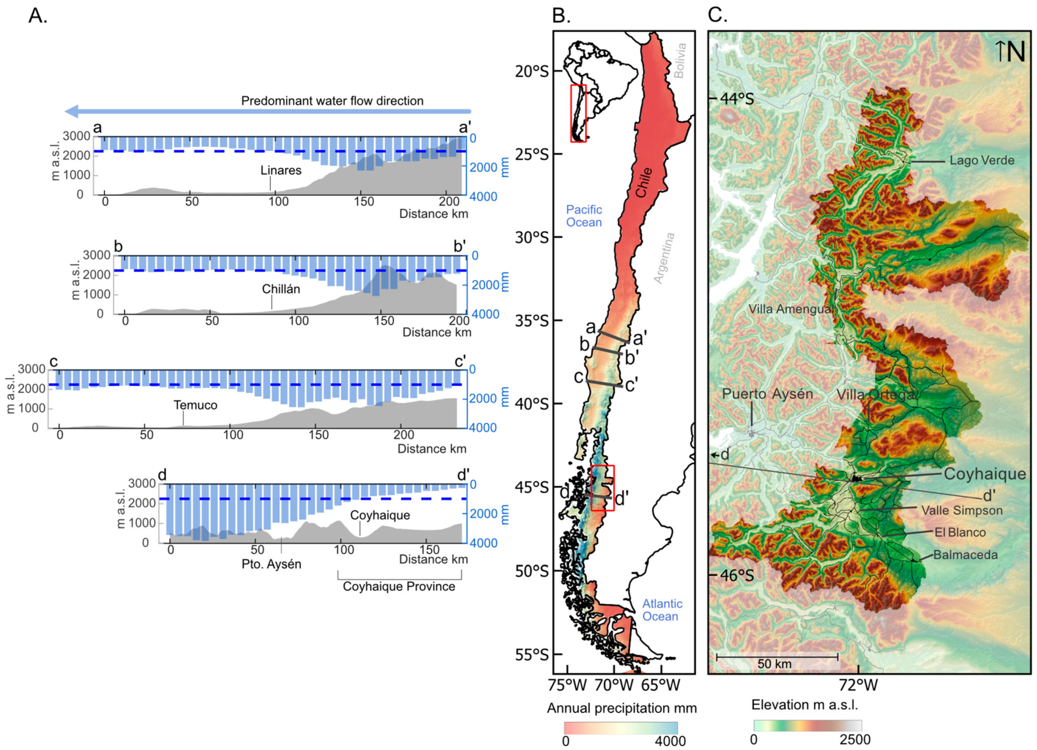
Figure 1. (A). West–east transects of elevation (m a.s.l.) and mean annual precipitation (mm) in the left-hand and right-hand axis respectively. (B). Overview of Chile’s annual precipitation (mm). Gray lines indicate transects on plot (A). (C). Elevation map of Coyhaique Province and main populated areas. Black lines indicate main roads.
Water 18 01041 g001
Figure 2. Water yield model. (A). Direct flow, (B). base flow, and (C). local recharge.
Water 18 01041 g002
Figure 3. (A). Anthropization index. (B). Water yield. (C). Water stress index. Points correspond to water intakes for human consumption (light-blue surficial water intakes and white groundwater intakes), and blue polygons correspond to their respective catchment.
Water 18 01041 g003
Table 2. Water stress index statistics.
WSI
Classification
Area (km2)Water Stress IndexWater Yield IndexAnthropization Index
MedianMinMaxMedianMinMaxMedianMinMax
High33360.690.601.000.070.000.550.500.251.00
Medium54250.510.410.600.150.000.820.130.000.75
Low37870.320.000.410.500.191.000.130.000.63
Disclaimer/Publisher’s Note: The statements, opinions and data contained in all publications are solely those of the individual author(s) and contributor(s) and not of MDPI and/or the editor(s). MDPI and/or the editor(s) disclaim responsibility for any injury to people or property resulting from any ideas, methods, instructions or products referred to in the content.