Machine Learning-Based Prediction of Irrigation Water Quality Index with SHAP Interpretability: Application to Groundwater Resources in the Semi-Arid Region, Algeria

Abstract

In semi-arid regions, sustainable groundwater management for irrigation is critical for agricultural productivity and food security. This study presents an integrated methodological framework combining hydrochemical characterization, machine learning (ML) modeling, and explainable artificial intelligence (XAI) to predict the Irrigation Water Quality Index (IWQI) in the Ain Oussera plain, Djelfa Province, Algeria. A total of 191 groundwater samples were collected from November 2023 to September 2024 and analyzed for major ions and physicochemical parameters. Multiple irrigation suitability indices were calculated, including Sodium Adsorption Ratio (SAR), Sodium Percentage (Na%), Magnesium Hazard (MH), Permeability Index (PI), Residual Sodium Carbonate (RSC), Soluble Sodium Percentage (SSP), and Kelly’s Ratio (KR). Five ML models were developed and evaluated for IWQI prediction: Random Forest, Gradient Boosting, XGBoost, K-Nearest Neighbors, and Support Vector Regression. Results showed that 55% of groundwater samples exhibited low to no restrictions for irrigation use, while 19% required high to severe restrictions. The XGBoost model demonstrated superior performance, with the highest R² (0.95) and the lowest RMSE (3.22) among all tested algorithms. SHAP (SHapley Additive exPlanations) analysis provided a transparent interpretation of model predictions, identifying electrical conductivity and Sodium Adsorption Ratio as the most influential parameters affecting IWQI, while chloride, sodium, total hardness, and magnesium had minimal impact. Spatial mapping using Inverse Distance Weighting (IDW) interpolation in ArcGIS 10.8 revealed considerable spatial variability in water quality throughout s the plain. This research addresses a critical gap in North African groundwater management by integrating ML predictive capabilities with XAI transparency, providing water resource managers and agricultural stakeholders with interpretable, data-driven tools for sustainable irrigation planning in water-stressed semi-arid environments.

1. Introduction

Groundwater resources represent the principal hydrological lifeline for agricultural irrigation in semi-arid regions globally, yet face unprecedented sustainability challenges from climate change, agricultural intensification, and overextraction. Recent global analyses indicate that 30% of regional aquifer systems have experienced accelerating depletion over the past four decades. This crisis is particularly acute in water-scarce regions where agriculture depends heavily on groundwater, with irrigation accounting for approximately 70% of global freshwater withdrawals [1]. In semi-arid zones, where limited rainfall and high evapotranspiration rates constrain surface water availability, groundwater quality directly determines agricultural viability, soil health, and food security. Inadequate water quality management in these contexts has cascading consequences for food production systems, rural livelihoods, and long-term environmental sustainability, demanding rigorous, integrated, and transparent assessment methodologies.

Irrigation water quality profoundly affects agricultural sustainability through multiple pathways. Poor quality irrigation water, characterized by excessive salinity, sodicity, or specific ion toxicity, can cause soil structure degradation, reduced infiltration capacity, nutrient imbalances, and ultimately crop failure [2]. While traditional single-parameter indices such as the Sodium Adsorption Ratio (SAR), Residual Sodium Carbonate (RSC), and Permeability Index (PI) have been widely used, they offer limited insights as they assess only isolated aspects of water quality and may yield contradictory results when applied simultaneously [3]. The Irrigation Water Quality Index (IWQI), developed by Meireles et al. [4], addresses these limitations by integrating five key parameters, electrical conductivity, sodium adsorption ratio, sodium, chlorides, and bicarbonates, into a single dimensionless indicator ranging from 0 to 100. This methodology has been extensively validated globally, with applications in Libya [5], Iraq [6,7], Brazil [8], India [9], Egypt [10,11], and Nigeria [12], demonstrating robust performance for agricultural water management decision support

The integration of machine learning (ML) algorithms into water quality assessment represents a paradigm shift from traditional empirical approaches to data-driven predictive modeling. Recent advances demonstrate that ensemble methods, notably Random Forest [13], Gradient Boosting [14], and extreme Gradient Boosting [15], consistently outperform traditional regression techniques for water quality prediction tasks, achieving high accuracy while handling noise and data variability [16], capturing complex non-linear relationships [17], and facilitating feature importance analysis [18]. Comprehensive reviews confirm that XGBoost achieves up to 94% accuracy compared to 67% for SVM in comparative studies [19], making ensemble methods the preferred choice for hydrochemical prediction tasks [20,21]. However, applications specifically targeting integrated irrigation quality indices in semi-arid regions remain limited, with most studies focusing on individual contaminants rather than composite IWQI prediction and lacking explainability methods for interpreting model outputs [22,23].

However, despite their high predictive accuracy, ML models function as “black boxes,” creating significant barriers to stakeholder trust and limiting scientific insight into the hydrochemical processes that govern water quality variability. This opacity is particularly problematic in environmental management, where regulatory compliance, public health protection, and resource allocation decisions require transparent, auditable, and justifiable predictions [24,25,26] developed SHAP (Shapley Additive exPlanations) as a rigorous game theoretic framework that decomposes each prediction into constituent feature contributions, enabling both global feature ranking and local prediction explanation. The TreeSHAP algorithm efficiently computes Shapley values for tree-based ensemble models, making SHAP practical for large groundwater datasets [24,27]. Recent applications demonstrate SHAP’s transformative potential. Choudhary et al. [27] achieved R² = 0.9952 using stacked ensemble regression with SHAP, while Makumbura et al. [24] employed SHAP-enhanced XGBoost (R² = 0.992) to identify oxygen demand parameters as dominant water quality drivers. Wu et al. [28] and Li et al. [29] further demonstrated SHAP’s effectiveness in identifying key regulatory parameters in diverse aquatic systems. By providing transparent, scientifically grounded insights, SHAP transforms machine learning from a black box tool into an actionable decision-support framework, enabling stakeholders to understand not only what a model predicts [30,31].

Algeria’s semi-arid regions face severe water stress driven by declining precipitation, rising evapotranspiration, agricultural intensification, and groundwater overexploitation. The Djelfa Province, characterized by limited annual rainfall (201–226 mm) and extensive agricultural activity, exemplifies these compounding challenges. Groundwater provisioning derives from five distinct hydrogeological units: the Ain Oussera Plain [32,33], the Zahrez Basin and Djelfa Syncline [34,35], the Barremian Plateau [36], and the Ain Ibel-Sidi Mekhlouf Syncline [37]. The Ain Oussera Plain, covering 3795 km² with agriculture dominated by arboriculture and fodder crops, exploits the Lower Albian sandstone as its principal aquifer (thickness 83–225 m, transmissivity 1.25 × 10⁻² m²/s to 0.50 × 10⁻³ m²/s). The aquifer is subject to contamination from agricultural activities, with elevated electrical conductivity, nitrate, and chloride levels documented by prior investigations [32]. Excessive pumping and evaporation represent compounding stressors contributing to progressive aquifer depletion [38,39]. Hydrochemical analyses in similar Algerian regions, the Oued Righ and Oued Souf, further highlight the vulnerability of these aquifers to agricultural and anthropogenic contamination [40,41].

Recent studies in Algerian regions demonstrate the feasibility of ML-based IWQI prediction. Zegaar et al. [42] applied ensemble methods integrated with SHAP for IWQI prediction in the M’sila region, while Hussein et al. [43] demonstrated strong XGBoost performance (R = 0.9834) in the Naama region. Gaagai et al. [44] showed that ANN models supported by GIS effectively assessed IWQI spatial variability in the Sahara aquifer, and Eid et al. [45] demonstrated the effectiveness of SVMR for IWQI prediction in the Souf Valley. However, comprehensive integration of hydrochemical characterization, advanced ML with rigorous hyperparameter optimization, SHAP-based interpretation, and GIS spatial analysis into a unified framework remains entirely absent for the Djelfa Province, the most agriculturally active yet least ML-explored semi-arid province in Algeria.

The present study addresses this critical methodological and regional gap. To the authors’ knowledge, no existing investigation for the Ain Oussera Plain simultaneously integrates multiparameter hydrochemical characterization, comparative evaluation of ML algorithms with rigorous hyperparameter optimization, multidimensional SHAP-based explainability, and GIS spatial analysis. This represents the first comprehensive application of explainable machine learning for IWQI prediction in Djelfa Province. This study, therefore, pursues the following specific objectives:

• Conduct comprehensive hydrochemical characterization and calculate irrigation suitability indices (SAR, RSC, MH, PI, KR, SSP, Na%) alongside IWQI for 191 groundwater samples collected across the Ain Oussera Plain during November 2023 to September 2024.
• Generate spatial distribution maps of water quality parameters and indices using GIS-based Inverse Distance Weighting (IDW) interpolation in ArcGIS.
• Develop, optimize, and compare five machine learning models, Support Vector Regression, K-Nearest Neighbors, Random Forest, Gradient Boosting, and XGBoost, for IWQI prediction from water quality parameters.
• Apply multidimensional SHAP analysis to interpret model predictions, quantify feature importance, and identify principal hydrochemical determinants of irrigation water quality.
• Provide actionable evidence-based recommendations for sustainable groundwater management and agricultural planning in the Ain Oussera Plain based on integrated hydrochemical–ML–SHAP–GIS insights.

2. Literature Review

2.1. Irrigation Water Quality Assessment and the IWQI Framework

The assessment of irrigation water quality has significantly evolved from single-parameter evaluations to more comprehensive multi-parameter indices. This shift reflects the need to capture the complex interactions that determine the suitability of water for agricultural purposes. Foundational guidelines by Ayers & Westcot [2] remain pivotal, focusing on salinity, sodium, and specific ion toxicities. However, traditional indices like Residual Sodium Carbonate (RSC), Permeability Index (PI), Magnesium Hazard (MH), and Sodium Adsorption Ratio (SAR) offer limited insights as they assess only single aspects of water quality. Recent assessments in semi-arid regions have demonstrated the critical importance of multi-parameter evaluation, as individual indices may present contradictory results. For instance, Yadav et al. [3] found that while SAR values were suitable primarily in India’s semi-arid river basin, the permeability index and magnesium hazard indicated that a significant percentage of water samples could degrade soil permeability and structure in the long term, with one-third of groundwater classified as unfit for irrigation despite acceptable SAR values.

Recent advancements have led to the development of integrated indices that provide a more holistic view of irrigation water suitability. The Irrigation Water Quality Index (IWQI), developed by Meireles et al. [4], addressed this limitation by integrating five critical parameters (EC, SAR, Na⁺, Cl⁻, HCO₃⁻) into a single dimensionless value (0–100) through weighted aggregation based on parameter importance for irrigation. The IWQI calculation involves: (1) computing quality scores (qi) for each parameter based on tolerance thresholds and categorical ranges; (2) applying empirically derived weights (wEC = 0.211, wNa = 0.204, wHCO₃ = 0.202, wCl = 0.194, wSAR = 0.189); (3) summing weighted quality scores to produce final IWQI classified into five restriction categories (No Restriction 85–100, Low Restriction 70–85, Moderate Restriction 55–70, High Restriction 40–55, Severe Restriction 0–40). This integrated approach is particularly valuable in semi-arid agricultural regions, where groundwater resources are subject to multiple quality stressors from natural hydrogeochemical processes and anthropogenic activities [3].

This methodology has been extensively validated globally across diverse contexts. Applications include Libya’s Al-Abyar area for evaluating government well water quality [5]; integrating IWQI with multivariate statistical methods to evaluate surface water quality for irrigation in Egypt’s Northern Nile Delta [11]; India’s Assam region, where multivariate IWQI categorized all locations as “Very Good” [9]; and India’s Bharalu River for long-term resource management [46]. Global applications demonstrate IWQI’s versatility: Nigeria’s Ekiti district for mapping farm settlement water quality under climate change [12]; Iraq’s major rivers (Tigris, Euphrates, Shatt al-Arab, Diyala) for assessing irrigation suitability [7]; India’s semi-arid river basin where hydrogeochemical analysis revealed high salinity and alkali hazards requiring integrated multi-parameter assessment [3], and Egypt’s Nile River where IWQI integration with ANN and PLSR models enhanced predictive capabilities [10].

Historically, Algerian studies have focused on traditional indices like SAR, RSC, and PI; however, recent research is beginning to incorporate IWQI integrated with machine learning approaches, reflecting a broader trend towards holistic water quality assessments. The work by Gaagai et al. [44], Eid et al. [45], Hussein et al. [43], and Zegaar et al. [42] marks significant steps in adopting IWQI and advanced predictive modeling in Algeria, demonstrating growing recognition of the benefits of integrated approaches for irrigation water quality management in semi-arid regions.

2.2. Machine Learning Applications in Groundwater Quality Prediction

The application of machine learning to water quality prediction has expanded significantly, driven by the need for more accurate and efficient methods to manage water resources. This shift is largely due to the superior performance of ML models over traditional statistical methods and the increasing availability of computational resources. The literature highlights the widespread adoption of various ML algorithms, such as Random Forest, Support Vector Machines, and Neural Networks, which have been effectively used to predict water quality parameters across different water bodies. Machine learning has been applied to groundwater management, including level prediction for irrigation support [47] and the prediction of quality parameters in semi-arid regions. Support Vector Machines have demonstrated strong performance for groundwater quality prediction, achieving R² = 0.92 (training) and R² = 0.87 (testing) for nitrate concentration in Iran’s Arak Plain using nine hydrochemical parameters from 160 samples across 40 wells [22], while neural networks have shown variable performance depending on architecture complexity, with deep neural networks (R² = 0.84) substantially outperforming standard three-layer architectures (R² = 0.64) for ammonium prediction using 322 samples across 55 wells [23], highlighting the importance of model selection for specific water quality parameters.

The transition towards hybrid and explainable models reflects growing interest in model interpretability and robustness. Popular algorithms, including Random Forest, XGBoost, LSTM, and CNN, are among the most frequently used for water quality prediction, offering high accuracy and adaptability to different datasets [19,20]. Ensemble methods have demonstrated superior performance, with XGBoost achieving 94% accuracy compared to 67% for SVM [19]. ML models have been applied to both surface and groundwater quality prediction, addressing various pollutants and quality indicators [48,49]. Rivers and aquifers are among the most studied water bodies, with models predicting key quality indicators such as WQI, DO, and nitrate concentrations [20]. However, applications in semi-arid regions remain limited, with most studies focusing on individual contaminants rather than integrated irrigation quality indices and lacking explainability methods such as SHAP for interpreting feature importance [22,23]. Recent comprehensive reviews emphasize the critical importance of data quality, method selection, and model validation for improving predictive accuracy in water quality applications [21].

2.3. Explainable AI and SHAP for Water Quality Model Interpretation

Despite their high predictive accuracy, machine learning models function as black boxes, creating barriers to adoption in environmental management contexts that require transparency for regulatory compliance, stakeholder trust, and scientific insight. Explainable AI (XAI), particularly SHAP (Shapley Additive exPlanations), has emerged as a critical solution for addressing these challenges in water quality prediction and broader environmental applications [24,30]. The growing adoption of XAI is evident from comprehensive reviews highlighting its effectiveness across environmental contexts, including water quality monitoring and climate science applications [30,31,50].

Applications of SHAP in water quality modeling have identified critical parameters as dominant drivers of predictions. Dissolved oxygen, BOD, conductivity, and pH emerged as key factors in WQI assessment [27], with additional studies identifying COD and BOD as most influential, while electrical conductivity showed minimal impact in certain contexts [24]. A comprehensive SHAP analysis across multiple ML algorithms identified pH, electrical conductivity, and major ions (Na, Ca, Mg, Cl, HCO₃, NO₃) as significant determinants of water quality classification [51]. This approach supports informed decision-making for sustainable water resource management [27,29].

The TreeSHAP algorithm calculates Shapley values efficiently for ensemble models based on decision trees (Random Forest, XGBoost, Gradient Boosting) by utilizing the structure of decision trees, rendering SHAP computation practical for extensive water quality datasets typically used in groundwater and surface water monitoring [24,27]. Despite these advances, challenges such as computational scalability and lack of standardized evaluation metrics persist, limiting widespread deployment in low-resource settings [30].

2.4. Research Gap

Despite advances in hydrochemical characterization, ML applications, and SHAP interpretability, significant methodological and regional gaps persist. Globally, and particularly in Algeria, no studies comprehensively integrate multi-parameter hydrochemical characterization with traditional indices (SAR, RSC, MH, PI, KR, SSP) and IWQI; comparative evaluation of multiple ML algorithms with rigorous hyperparameter optimization; SHAP-based explainability for both global and local interpretation; and GIS-based spatial analysis.

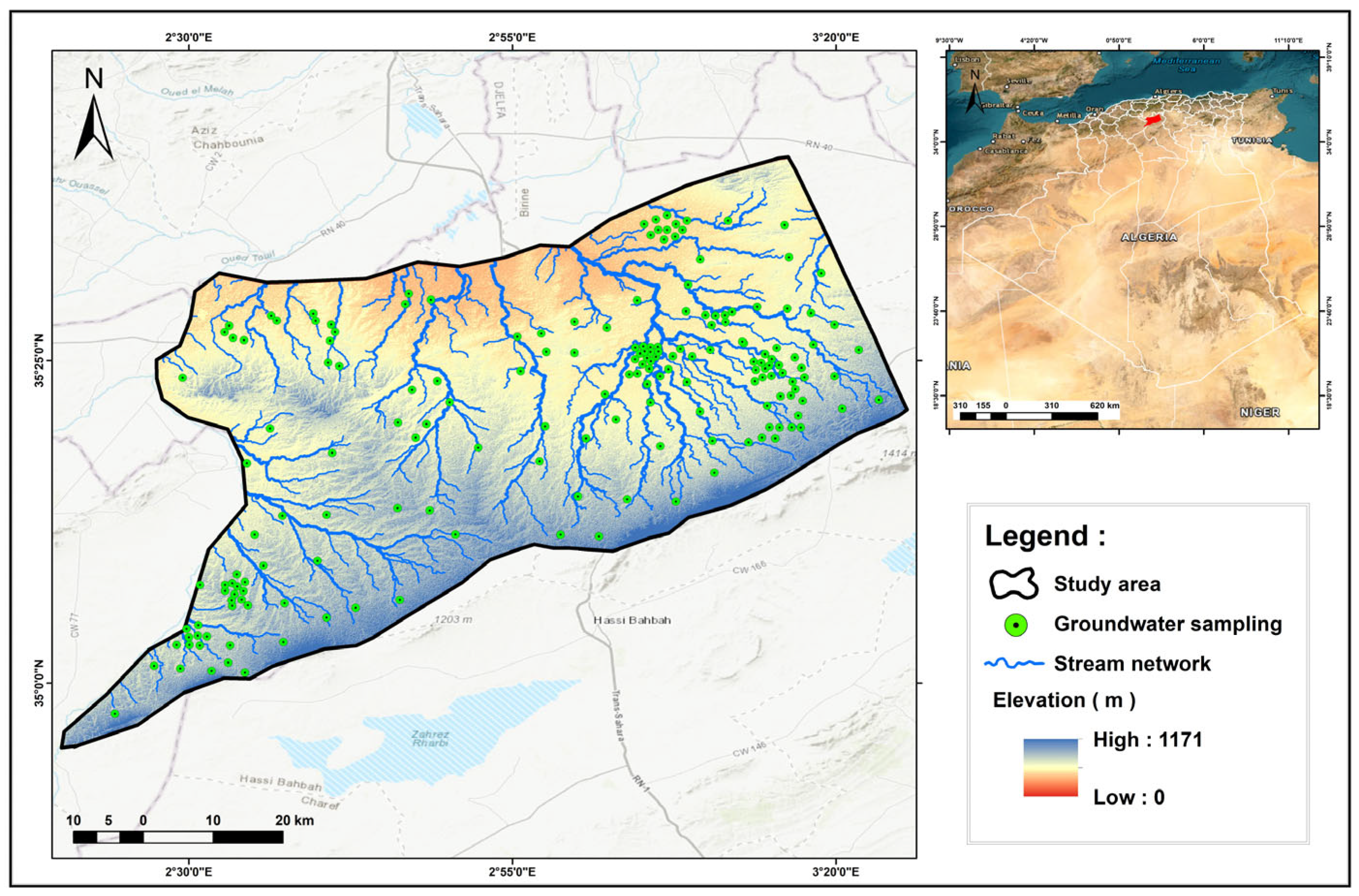
The Djelfa Province, specifically Ain Oussera Plain, significantly lacks ML-based water quality prediction studies despite its strategic importance for agricultural water supply, documented water quality concerns (elevated EC, nitrates, chlorides) [52], semi-arid climate vulnerability (226 mm/year precipitation), and systematic prior hydrogeological characterization providing a foundation for ML advancement. While [42] and [43] pioneered SHAP applications in M’sila and Naama regions, respectively, SHAP-based IWQI interpretation for Djelfa Province remains absent, and most Algerian groundwater studies employ static assessments with limited temporal scope, constraining predictive capacity for ungauged locations and future scenarios. This study addresses these gaps through an integrated hydrochemical-ML-SHAP-GIS analysis of the Ain Oussera Plain (Figure 1), representing the first comprehensive application of explainable machine learning for IWQI prediction in Djelfa Province and advancing the methodological state of the art for Algerian semi-arid water resource management.

3. Materials and Methods

3.1. The Description of the Study Area

The Ain Oussera Plain is situated in the central part of northern Algeria, within the Algerian High Plains of Djelfa province, approximately 200 km south of Algiers, bounded by latitudes 35°00′–35°40′ north and longitudes 2°15′–3°45′ east, structurally delimited by the Saharan Atlas to the south and the Maghrebian chain to the north [53].

The study area covers approximately 3795 km², forming an elongated east–west-oriented strip extending about 110.2 km in length and 46 km in width between the towns of Birine and Taguine, with average elevations ranging from 632 to 900 m (Figure 1). Climatically, the area falls within the semi-arid zone, characterized by hot, dry summers and cool-to-cold winters. The average annual rainfall is about 226.15 mm, and the mean annual temperature is 17.6 °C [52]. The plain contains several aquifer formations with varying hydraulic potentials, including Quaternary deposits, Miocene sandstones, and limestones from the Lower Eocene, Turonian, and Cenomanian, as well as Albo-Barremian sandstones [54,55]. Among these, the Albian aquifer constitutes the most important groundwater reservoir in the region. It is exploited through numerous boreholes used to supply drinking water to towns and to support agricultural activities. The Lower Albian sandstones form the primary aquifer within the study area. This is an unconfined aquifer extending over a large area, with a thickness ranging from 83 to 225 m, and an average thickness of about 150 m. The transmissivity ranges from 1.25 × 10⁻² m²/s to 0.50 × 10⁻³ m²/s, with higher values recorded in the northeastern part of the study zone. The permeability shows a similar spatial distribution pattern to transmissivity, with values ranging from 1.0 × 10⁻⁶ m/s to 4.3 × 10⁻⁴ m/s. The storage coefficient is estimated between 0.93 × 10⁻³ and 1.3 × 10⁻³ [39,56].

Agricultural production in the Ain Oussera region is almost exclusively reliant on groundwater abstracted from the Albian aquifer, owing to the near-total absence of perennial surface water resources under prevailing semi-arid climatic conditions. Since the early 2000s, the successive implementation of national agricultural development schemes, namely the FNRDA (Fonds National de Régulation et Développement Agricole) and FNDIA (Fonds National de Développement et d’Investissement Agricole, has driven a substantial expansion of irrigated cropland, placing mounting pressure on groundwater reserves and resulting in a sustained decline of piezometric levels documented over more than three decades of hydrological monitoring. Irrigated cultivation is spatially concentrated on the Sersou plateau and in the areas southwest of Birine, where annual crops constitute the primary land use under irrigation. Arboricultural systems, notably orchards of apple, pear, and olive, along with forage crops including sorghum and alfalfa, represent the dominant agricultural land uses, while horticultural production remains marginal and geographically restricted. The progressive intensification of farming practices has engendered a multi-source groundwater contamination dynamic. The indiscriminate application of nitrogenous fertilizers has resulted in nitrate enrichment exceeding 75 mg/L in the Had Sahary sector and surpassing Algerian regulatory thresholds (50 mg/L) in the Guernini zone [52].

3.2. Data Collection and Description

For this study, 191 groundwater samples were collected from the Ain Oussera Plain, spanning from November 2023 to September 2024. The sampling sites were deliberately chosen to ensure uniform spatial coverage of the plain. The sampling campaign provided a multi-season dataset that captures temporal variability in groundwater chemistry linked to recharge cycles and agricultural practices. The study area includes several boreholes ranging in depth from 100 to 300 m, with aquifer thicknesses of 83 to 225 m, tapping the deep sandstone formations of the plain. To assess water quality, 11 physicochemical parameters were measured according to standard analytical procedures. Before collecting samples, all containers were carefully rinsed with distilled water to prevent contamination. Each well or borehole was purged for 5 to 10 min prior to sampling to remove stagnant water, ensuring that the collected samples accurately reflected the actual in situ groundwater conditions.

Physical properties, including pH and electrical conductivity (EC), were measured on-site using calibrated field instruments in accordance with standard procedures. For chemical analysis, the samples were sent to an accredited laboratory of the Algerian Water Authority (ADE). Chemical analysis targeted four major cations (Na⁺, Ca²⁺, Mg²⁺, K⁺) and four major anions (Cl⁻, SO₄²⁻, HCO₃⁻, NO₃⁻). Different analytical techniques were applied depending on the ion: EDTA titration for calcium, magnesium, and total hardness; flame photometry for sodium and potassium; titration for chlorides and bicarbonates; and spectrophotometry for sulfates and nitrates. Strict quality assurance and quality control (QA/QC) protocols were followed throughout the laboratory analysis. To detect and correct potential sources of error, procedural blank measurements and sample spiking with known analyte concentrations were performed. To ensure reproducibility, all observations were recorded in duplicate, and average values were reported as final results. The ionic balance of each sample was calculated to verify the reliability of the analytical results, with an acceptable ionic balance error not exceeding ±5%. The suitability of groundwater for irrigation in the Ain Oussera Plain was assessed according to the Food and Agriculture Organization (FAO) guidelines. A summary of the descriptive statistics for all measured water quality parameters is provided in

Table 1. Descriptive Statistics of Water Quality Parameters.

Parameter	Min	Max	Mean	Std	Skewness	Kurtosis
pH	6.82	8.80	7.63	0.45	0.75	−0.41
CE (us/cm)	421.00	3800.00	1653.77	910.45	0.90	−0.31
Ca (mg/L)	17.00	397.70	105.41	68.61	1.48	2.29
Mg (mg/L)	8.00	711.70	72.83	64.04	6.05	56.19
Na (mg/L)	17.50	906.00	128.76	121.28	3.41	16.58
K (mg/L)	1.50	72.00	7.85	9.12	4.25	21.49
Cl (mg/L)	19.97	1650.00	256.65	233.06	2.90	13.17
SO4 (mg/L)	7.08	2800.00	271.36	314.48	4.02	24.81
TH (F)	14.75	351.29	56.70	37.93	3.28	20.89
HCO3 (mg/L)	6.00	1418.00	229.11	141.99	4.88	33.24
NO3 (mg/L)	0.01	82.60	30.31	21.46	0.74	−0.48

.

3.3. Suitability Indices for Irrigation

Agricultural groundwater quality was evaluated through a comprehensive multi-parametric analysis that combined various indicators, such as the Sodium Adsorption Ratio (SAR), Sodium Percentage (Na%), Magnesium Hazard Index (MH), Soluble Sodium Percentage (SSP), Residual Sodium Carbonate (RSC), Permeability Index (PI), and Kelly’s Ratio (KR). These indicators permit a holistic assessment of irrigation water quality. Equations (1)–(7) [57,58,59,60,61,62,63] were calculated using the standard formulas mentioned below to compute, respectively. Ionic concentrations used to determine SAR, Na%, MH, SSP, RSC, PI, and KR were expressed as milliequivalents per liter (meq/L).

$$\mathrm{S}\mathrm{A}\mathrm{R}={\displaystyle \frac{{\mathrm{N}\mathrm{a}}^{+}}{\sqrt{\frac{{\mathrm{C}\mathrm{a}}^{2+}+{\mathrm{M}\mathrm{g}}^{2+}}{2}}}}$$

(1)

$$\mathrm{N}\mathrm{a}\mathrm{\%}={\displaystyle \frac{\left({\mathrm{N}\mathrm{a}}^{+}+{\mathrm{K}}^{+}\right)}{\left({\mathrm{C}\mathrm{a}}^{2+}+{\mathrm{M}\mathrm{g}}^{2+}+{\mathrm{N}\mathrm{a}}^{+}+{\mathrm{K}}^{+}\right)}}\times 100$$

(2)

$$\mathrm{M}\mathrm{H}={\displaystyle \frac{\left({\mathrm{M}\mathrm{g}}^{2+}\right)}{\left({\mathrm{C}\mathrm{a}}^{2+}+{\mathrm{M}\mathrm{g}}^{2+}\right)}}\times 100$$

(3)

$$\mathrm{S}\mathrm{S}\mathrm{P}={\displaystyle \frac{\left({\mathrm{N}\mathrm{a}}^{+}\right)}{\left({\mathrm{N}\mathrm{a}}^{+}+{\mathrm{C}\mathrm{a}}^{2+}+{\mathrm{M}\mathrm{g}}^{2+}\right)}}\times 100$$

(4)

$$\mathrm{R}\mathrm{S}\mathrm{C}=({\mathrm{HCO}}_3^{-}+{\mathrm{CO}}_3^{-2})-({\mathrm{Ca}}^{2+}+{\mathrm{Mg}}^{2+})$$

(5)

$$\mathrm{P}\mathrm{I}={\displaystyle \frac{\left({\mathrm{N}\mathrm{a}}^{+}+\sqrt{{\mathrm{H}\mathrm{C}\mathrm{O}}_3^{-}}\right)}{\left({\mathrm{C}\mathrm{a}}^{2+}+{\mathrm{M}\mathrm{g}}^{2+}+{\mathrm{N}\mathrm{a}}^{+}\right)}}\times 100$$

(6)

$$\mathrm{K}\mathrm{R}={\displaystyle \frac{{\mathrm{N}\mathrm{a}}^{+}}{{\mathrm{C}\mathrm{a}}^{2+}+{\mathrm{M}\mathrm{g}}^{2+}}}$$

(7)

3.4. Irrigation Water Quality Index (IWQI)

Effective groundwater quality management is crucial for sustainable agriculture in arid and semi-arid regions, where irrigation predominantly relies on these water resources. The suitability of groundwater for irrigation is influenced by its mineral composition and its impact on the soil–plant system [64]. Excessive mineralization can adversely affect crop productivity through two primary mechanisms: (i) elevated salinity increases the osmotic pressure in the soil solution, directly impairing plant physiological processes and growth, and (ii) alterations in soil physical properties, such as structure, permeability, and aeration, induced by the chemical composition of the water, indirectly affect plant development [43]

The Irrigation Water Quality Index (IWQI) is a dimensionless indicator that evaluates water suitability for irrigation by integrating its chemical composition [65]. This method synthesizes information from five key parameters, including electrical conductivity (EC), sodium adsorption ratio (SAR), sodium (Na⁺), chlorides (Cl⁻), and bicarbonates (HCO₃⁻), into a single value ranging from 0 to 100. The calculation process involves weighting each parameter by its importance for irrigation, followed by a mathematical aggregation to produce an overall score, with higher values indicating better water quality for agricultural use. In the current methodology, each parameter’s quality score (q_i) is computed using Equation (8), with the tolerance thresholds from

Table 2. Limiting values for parameters used in quality assessments (q_i).

qi	EC (µs/cm)	Na (meq/L)	Cl (meq/L)	HCO3 (meq/L)	SAR (meq/L)1/2
85–100	0.2 ≤ EC < 0.75	2 ≤ Na < 3	1 ≤ Cl < 4	1 ≤ HCO3 < 1.5	2 ≤ SAR < 3
60–85	0.75 ≤ EC < 1.50	3 ≤ Na < 6	4 ≤ Cl < 7	1.5 ≤ HCO3 < 4.5	3 ≤ SAR < 6
35–60	1.50 ≤ EC < 3.00	6 ≤ Na < 12	7 ≤ Cl < 10	4.5 ≤ HCO3 < 8.5	6 ≤ SAR < 12
0–35	EC < 0.2 or EC ≥ 3.0	Na < 2 or Na ≥ 12	Cl < 1 or Cl ≥ 10	HCO3 < 1 or HCO3 ≥ 8.5	SAR < 2 or SAR ≥ 12

.

$${\mathrm{q}}_{\mathrm{i}}={\mathrm{q}}_{\mathrm{m}\mathrm{a}\mathrm{x}}-\left({\displaystyle \frac{\left[\left({\mathrm{x}}_{\mathrm{i}\mathrm{j}}-{\mathrm{x}}_{\mathrm{i}\mathrm{n}\mathrm{f}}\right){\mathrm{q}}_{\mathrm{i}\mathrm{a}\mathrm{m}\mathrm{p}}\right]}{{\mathrm{x}}_{\mathrm{a}\mathrm{m}\mathrm{p}}}}\right)$$

(8)

where q_i represents the quality score of the i-th parameter, q_max is the maximum permissible score, x_ij is the observed value for each parameter, x_inf is the lower threshold for the parameter class, q_iamp denotes the class-specific amplitude of the quality score, and x_amp represents the total range of the parameter class.

The final Irrigation Water Quality Index (IWQI) for each groundwater sample established by [4] and detailed in

Table 3. Relative weighting coefficients for IWQI computation.

Indicator	wi
EC	0.211
Na	0.204
HCO3	0.202
Cl	0.194
SAR	0.189
Total	1.000

was computed using a weighted aggregation approach, as shown in Equation (9):

$$\mathrm{I}\mathrm{W}\mathrm{Q}\mathrm{I}={\sum }_{\mathrm{i}=1}^{\mathrm{n}}{\mathrm{q}}_{\mathrm{i}}\mathrm{x}{\mathrm{w}}_{\mathrm{i}}$$

(9)

where qᵢ represents the individual quality score of the i-th parameter, and wᵢ denotes the relative weighting assigned to that parameter based on its importance for irrigation.

The IWQI is available in the range of 0 to 100. As illustrated in

Table 4. Classification of IWQI) and corresponding water use Restrictions.

IWQI	Water Use Restrictions
0–40	Severe restriction [SR]
40–55	High restriction [HR]
55–70	Moderate restriction [MR]
70–85	Low restriction [LR]
85–100	No restriction [NR]

, the irrigation water quality index (IWQI) was classified into five (05) categories, ranging from excellent to inappropriate.

3.5. Data Preprocessing

Data preprocessing is a critical step in any machine learning pipeline, as it directly conditions the quality and reliability of predictive models. In this study, a rigorous multi-step preprocessing framework was applied to the raw hydrochemical dataset prior to model training.

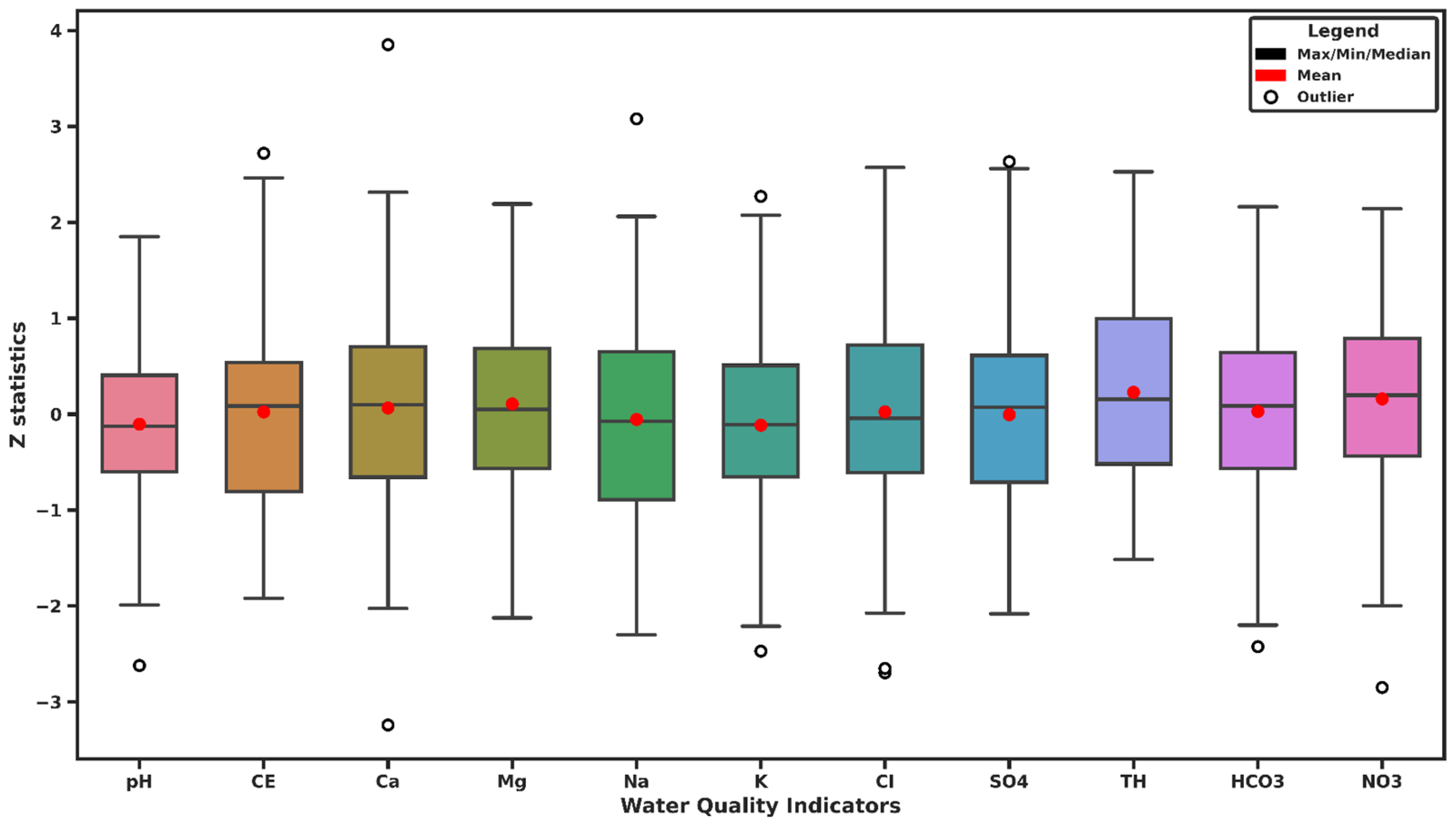
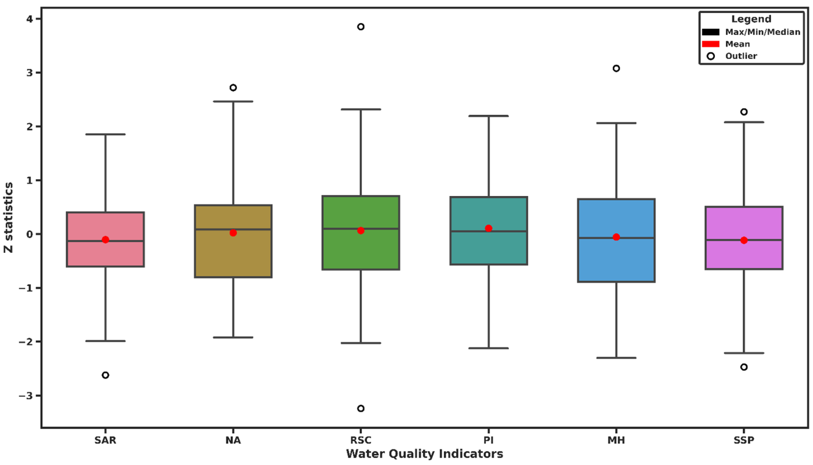
The reliability of the physicochemical dataset was first assessed using two complementary approaches: ionic balance verification and box plot visualization. The ionic balance (IB) was calculated for each sample, and those exceeding the ±5% threshold were eliminated following standard hydrochemical quality control procedures. Box plots (Figure 2) provided an initial visual screening of parameter distributions and extreme values. Subsequently, a completeness audit confirmed that the dataset contained no missing values across all samples and physicochemical parameters, a result attributable to the strict QA/QC protocols maintained throughout the field sampling campaign and laboratory analysis. The preprocessing pipeline was then executed in the following strict sequential order: (1) outlier detection and removal using statistical quantiles, followed by appropriate transformation where necessary; (2) random partitioning of the cleaned dataset into a training set (80%) and a test set (20%), performed prior to any scaling operation; (3) computation of Min-Max scaling parameters, specifically x min and x max, derived exclusively from the training set; and (4) application of these training derived parameters to normalize the test set, according to Equation (10):

$$X_{norm}={\displaystyle \frac{x-x_{min}}{x_{max}-x_{min}}}$$

(10)

$$IB\left(\%\right)=\left|{\displaystyle \frac{\sum Cations-\sum Anions}{\sum Cations+\sum Anions}}\times 100\right|$$

(11)

3.6. Geospatial Analysis

Geographic Information Systems (GIS) were used to analyze and manage groundwater quality across the study area. GIS helps map spatial patterns, assess environmental risks, and support decision-making at both local and regional levels. In this study, the spatial distribution of key groundwater parameters such as electrical conductivity (EC), sodium (Na), chloride (Cl), and bicarbonate (HCO₃), as well as water quality indices including SAR, PI, Na%, SSP, RSC, MH, KR, and the Irrigation Water Quality Index (IWQI), were examined. The Inverse Distance Weighting (IDW) interpolation method in ArcGIS was applied to generate spatial maps of all parameters. IDW was chosen because it is widely recognized as suitable for interpolating groundwater quality data and for effectively capturing spatial trends [52,66]

3.7. Violin and Box Plot Visualization Methods

In this study, violin plots and box plots were employed as complementary visualization techniques for comprehensive distributional analysis of water quality parameters. Violin plots were utilized to combine box plot summary statistics with kernel density estimation (KDE), thereby revealing distributional shape, spread, and multimodality through symmetrical density curves. Concurrently, box plots were implemented to provide concise five-number summaries (minimum, first quartile Q₁, median, third quartile Q₃, and maximum), wherein the interquartile range (IQR) box delineates the central 50% of observations, whiskers capture remaining variability, and discrete markers identify potential outliers exceeding the whisker boundaries. This dual visualization approach facilitated robust exploratory data analysis and enhanced the detection of distributional anomalies in the dataset.

3.8. Feature Selection

3.8.1. Correlation Analysis

We employed correlation analysis to investigate the relationships between various groundwater quality parameters and the Irrigation Water Quality Index (IWQI). The Pearson correlation coefficient (r) was used to quantify the strength and direction of linear relationships between continuous variables, with values ranging from −1 to +1. A positive correlation means that both values increase together; a negative correlation means that one increases while the other decreases; and a value close to zero indicates almost no relationship. Statistical significance of correlations was assessed according to the criteria outlined by Chan [67], Dancey & Reidy [68]. The important parameters identified from this step were then used as inputs for machine learning models to better understand what drives groundwater quality for irrigation.

3.8.2. Recursive Feature Elimination with Cross-Validation (RFECV)

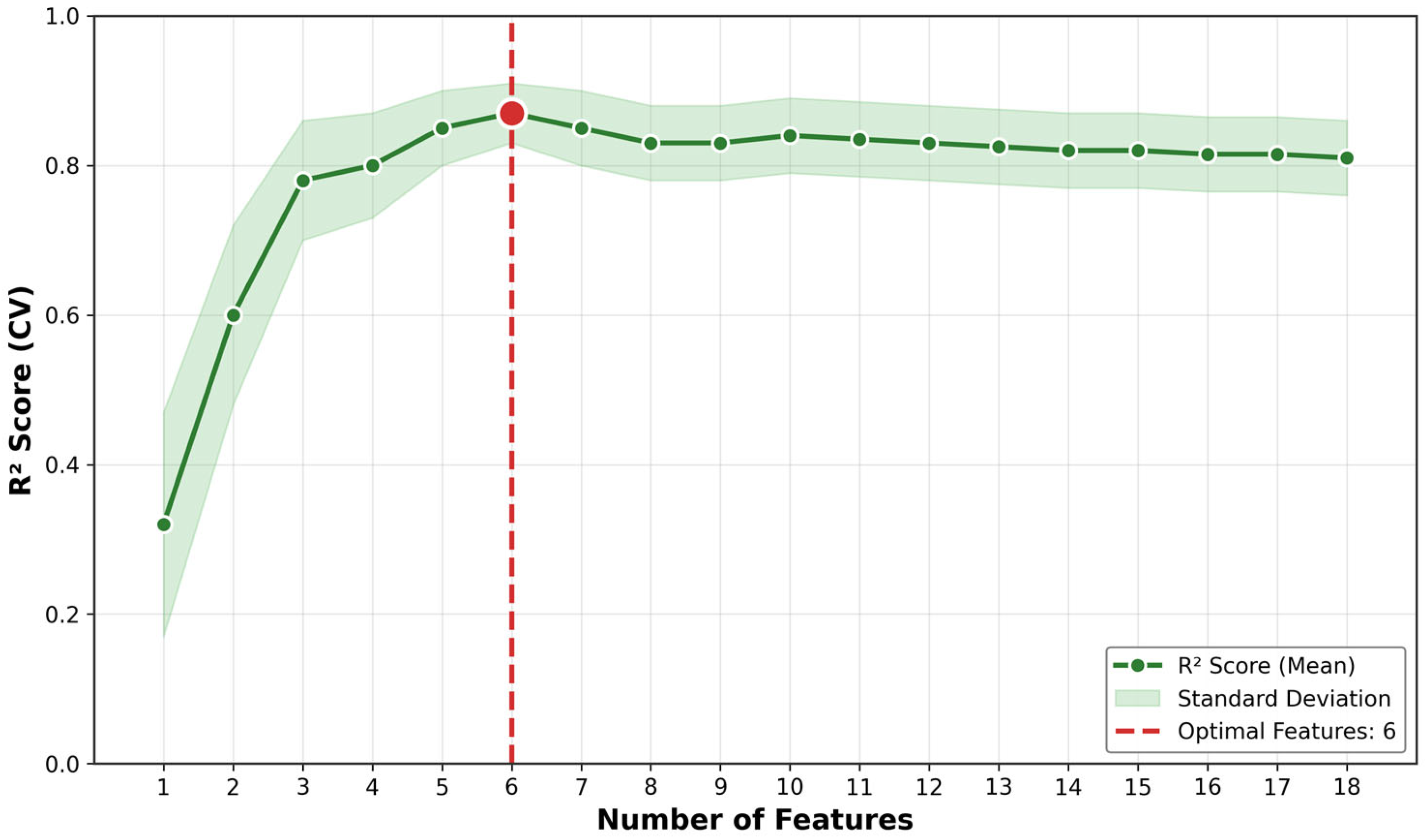
To identify critical predictors for IWQI modeling, the RFECV algorithm was employed. This technique is widely recognized for its effectiveness in identifying the most relevant predictors by iteratively removing less significant features and evaluating model performance at each step [69,70]. The parameters retained by RFECV were further validated against hydrogeochemical theory: each of the six selected variables (EC, Na⁺, Cl⁻, SAR, TH, Mg²⁺) corresponds to a distinct dimension of the IWQI formula, salinity, sodicity, specific ion toxicity, and hardness, confirming that the data-driven dimensionality reduction is consistent with the established hydrochemical framework governing irrigation suitability assessment [4]. In this study, RFECV was applied using the scikit-learn implementation [71], combined with a Random Forest (RF) regressor as the base estimator due to its robustness against multicollinearity and its ability to handle nonlinear relationships among groundwater parameters [42,72]. The algorithm began with all selected features from correlation analysis, and then recursively eliminated the least essential variable based on model coefficients or feature importance scores. At each iteration, k-fold cross-validation (k = 5) was performed to estimate model performance, ensuring that the optimal number of features was selected based on the highest average cross-validated coefficient of determination (R²). The final number of features was chosen at the point where model accuracy stopped improving. This approach helped to find the most useful parameters while keeping the model simple and efficient.

3.9. Machine Learning Model

Five machine learning algorithms were selected to represent a comprehensive and complementary spectrum of learning paradigms: Support Vector Regression (SVR) as a kernel-based approach suited for small-to-medium hydrochemical datasets; K-Nearest Neighbors (KNN) as an instance-based non-parametric benchmark; and Random Forest (RF), Gradient Boosting (GB), and XGBoost as tree-based ensemble methods recognised in the literature for superior performance on tabular hydrochemical data characterised by non-linear parameter interactions [13,14,15]. This multi-paradigm design enables rigorous comparative evaluation and isolates the specific performance gain attributable to ensemble architecture, consistent with recent Algerian groundwater ML studies [42,43].

3.9.1. Support Vector Regression (SVR)

Support Vector Regression is a machine learning technique derived from the Support Vector Machine (SVM) algorithm, specifically adapted for regression and continuous-variable prediction. Initially developed by Vapnik et al. [73], SVR is distinguished by its ability to handle nonlinear data and complex relationships [74]. Its operation is based on finding an optimal hyperplane in a multidimensional space, maximizing the margin while keeping prediction errors within acceptable limits [73]. This methodology enables the model to accurately predict continuous variables by applying the core concepts of support vector machines. The SVR prediction function for nonlinear relations, we use a different kernel, and display:

$$\widehat{\mathrm{y}}\left(\mathrm{x}\right)={\sum }_{\mathrm{i}=1}^{\mathrm{m}}({\mathsf{\alpha }}_{\mathrm{i}}-{{\mathsf{\alpha }}^{\mathrm{\ast }}}_{\mathrm{i}})\mathrm{K}\left({\mathrm{x}}_{\mathrm{i}},\mathrm{x}\right)+\mathrm{b}$$

(12)

${\mathsf{\alpha }}_{\mathrm{i}},{{\mathsf{\alpha }}^{\mathrm{\ast }}}_{\mathrm{i}}$: Learning multipliers; K (${\mathrm{x}}_{\mathrm{i}},\mathrm{x}$): kernel function linear, rbf, polynomial, and linear ${\mathrm{x}}_{\mathrm{i}}$: Support vectors; b: bias term

The SVR optimization format equation would be:

$${\mathrm{m}\mathrm{i}\mathrm{n}}_{\mathrm{w},\mathrm{b},{\mathsf{\epsilon }}_{\mathrm{i}},{\mathsf{\epsilon }}_{\mathrm{i}\mathrm{\ast }}}{\displaystyle \frac{1}{2}}{\left|\left|\mathrm{w}\right|\right|}^2+\mathrm{C}{\sum }_{\mathrm{i}=1}^{\mathrm{m}}({\mathsf{\epsilon }}_{\mathrm{i}}+{\mathsf{\epsilon }}_{\mathrm{i}}^{\mathrm{\ast }})$$

(13)

$$\begin{array}{cc}\mathrm{Subjected} \mathrm{to}:\hspace{1em}\hspace{1em}\hfill & {\mathrm{y}}_{\mathrm{i}}-{\mathrm{w}}^{\mathrm{T}}{\mathrm{x}}_{\mathrm{i}}-\mathrm{b}\le \mathsf{\epsilon }+{\mathsf{\epsilon }}_{\mathrm{i}}\\ & {\mathrm{w}}^{\mathrm{T}}{\mathrm{x}}_{\mathrm{i}}+\mathrm{b}-{\mathrm{y}}_{\mathrm{i}}\le \mathsf{\epsilon }+{\mathsf{\epsilon }}_{\mathrm{i}}^{\mathrm{\ast }}\\ & {\mathsf{\epsilon }}_{\mathrm{i}}{\mathsf{\epsilon }}_{\mathrm{i}}^{\mathrm{\ast }}\ge 0\end{array}$$

• C: controls penalty for large errors
• $\mathsf{\epsilon }$: width of tolerance zone
• $\mathsf{\epsilon },{\mathsf{\epsilon }}_{\mathrm{i}}^{\mathrm{\ast }}$: slack variables for errors outside the $\mathsf{\epsilon } \mathrm{t}\mathrm{u}\mathrm{b}\mathrm{e}$

3.9.2. Random Forests

The Random Forest method, developed by [13], represents a significant advancement in machine learning. The technique develops multiple autonomous decision trees and integrates their results. Its robustness increases with the number of trees, thereby reducing the risk of overfitting. The process comprises two essential phases: constructing multiple trees and using them collectively for prediction [75,76]. In Random Forests, predictions are obtained by aggregating the outputs of all decision trees. For classification tasks, the model selects the majority class, while for regression tasks, it averages the predictions of individual trees. Mathematically, these can be represented as:

$$\begin{gathered} \mathrm{For} \mathrm{Classification}:\mathrm{H}(\mathrm{X})=\mathrm{mode} \{{\mathrm{h}}_1(\mathrm{X}), {\mathrm{h}}_2(\mathrm{X})\dots {\mathrm{h}}_{\mathrm{k}}(\mathrm{X})\}; \\ \mathrm{For} \mathrm{Regression}: \mathrm{f}(\mathrm{X})={\displaystyle \frac{1}{B}}{\sum }_{b=0}^B{f}_b\left(X\right); \end{gathered}$$

where H(X) is the final prediction, h_k(X) is the prediction of tree k, B is the total number of trees, F_b(X) is the prediction of tree b.

3.9.3. K-Nearest Neighbours (KNN) Algorithm

KNN is a supervised learning method that stands out for its simplicity and effectiveness in classification and regression tasks. Its uniqueness lies in its nonparametric approach, in which predictions are based directly on existing data without prior assumptions about their distribution [77]. Its operation relies on analyzing the K nearest neighbors of a given point, where K is a crucial parameter that directly influences the model’s performance depending on the data being processed [43,78]. The equation:

$$\mathrm{d}\left({\mathrm{x},\mathrm{x}}_{\mathrm{i}}\right)=\sqrt{{\sum }_{\mathrm{j}=1}^{\mathrm{n}}{\left({\mathrm{x}}_{\mathrm{j}}-{\mathrm{x}}_{\mathrm{i}\mathrm{j}}\right)}^2}$$

(14)

For the regression process, the equation would only become an average of the k nearest points:

$$\widehat{\mathrm{y}}={\displaystyle \frac{1}{\mathrm{k}}}{\sum }_{\mathrm{i}\in {\mathrm{N}}_{\mathrm{K}\left(\mathrm{x}\right)}}{\mathrm{y}}_{\mathrm{i}}$$

(15)

${\mathrm{N}}_{\mathrm{K}\left(\mathrm{x}\right)}$: set of the K nearest neighbours to x.

3.9.4. Gradient Boosting

Introduced by [14], Gradient Boosting constitutes an advanced ensemble learning approach suitable for both regression and classification applications. The core methodology centers on developing a strong predictive system by progressively assembling multiple weak predictors, typically decision tree structures, wherein each subsequent component targets the correction of prediction errors from earlier ensemble members [42]. This progressive enhancement strategy efficiently minimizes a selected loss function and achieves higher predictive accuracy, including in scenarios involving complex nonlinear patterns. At every stage, Gradient Boosting introduces a new weak predictor calibrated to forecast the residuals (prediction errors) from the preceding model configuration rather than the raw response variable. The cumulative prediction emerges from synthesizing all weak predictors, modulated by a learning rate coefficient (γ_m/gamma) that determines the magnitude of each new predictor’s influence on the aggregate model. The algorithmic representation at the mth optimization step is given by:

F_m(x) = F_m−1(x) + γ_mh_m(x)

(16)

where F_m(x) is the model at step m, γ_m is the learning rate, and h_m(x) is the weak learner.

3.9.5. Extreme Gradient Boosting

XGBoost is an advanced, computationally efficient ensemble learning algorithm that builds on conventional Gradient Boosting frameworks. The technique amalgamates outputs from multiple weak predictors, typically decision tree architectures, to generate a powerful and accurate predictive system. Unlike standard boosting methods, XGBoost employs a regularized objective function that curtails overfitting and improves the model’s generalization [15]. Its reputation stems from exceptional scalability and computational performance, making it well-suited for handling extensive datasets with high-dimensional feature spaces. The algorithm operates through iterative tree generation, where each new tree aims to rectify residual errors from prior iterations while fine-tuning performance via hyperparameter optimization, including learning rate, maximum tree depth, and regularization parameters.

XGBoost = Gradient Boosting + Regularization + Efficient Tree Building was the objective equation:

$$\mathrm{O}\mathrm{b}\mathrm{j}={\sum }_{\mathrm{i}=1}^{\mathrm{n}}\mathrm{L}({\mathrm{y}}_{\mathrm{i}},{\widehat{\mathrm{y}}}_{\mathrm{i}})+{\sum }_{\mathrm{t}=1}^{\mathrm{T}}\mathrm{G}\left({\mathrm{f}}_{\mathrm{t}}\right)$$

(17)

L: the training loss

G: the regularization term that penalizes complex trees

3.10. Model Evaluation

Several statistical measures were applied to assess the machine learning algorithms’ ability to estimate the Irrigation Water Quality Index (IWQI). Root Mean Squared Error (RMSE) quantifies the average magnitude of prediction errors, giving higher weight to larger deviations. It is calculated as:

$$\mathrm{R}\mathrm{M}\mathrm{S}\mathrm{E}=\sqrt{{\displaystyle \frac{1}{\mathrm{n}}}{\sum }_{\mathrm{i}=1}^{\mathrm{n}}{{(\mathrm{y}}_{\mathrm{i}}-{\mathrm{y}}_{\mathrm{p}})}^2}$$

(18)

where y_i and y_p represent the observed and predicted IWQI values, respectively, and n is the total number of samples.

Mean Absolute Error (MAE) measures the average absolute differences between predicted and actual values, calculated as:

$$\mathrm{M}\mathrm{A}\mathrm{E}={\displaystyle \frac{1}{\mathrm{n}}}\sqrt{{\sum }_{\mathrm{i}=1}^{\mathrm{n}}|{\mathrm{y}}_{\mathrm{i}}-{\mathrm{y}}_{\mathrm{p}}|}$$

(19)

Lower values of RMSE and MAE indicate better predictive accuracy.

The coefficient of determination (R²) measures the extent of IWQI variability captured by the independent variables and is formulated as:

$${\mathrm{R}}^2=1-{\displaystyle \frac{\frac{1}{\mathrm{n}}\sum _{\mathrm{i}=1}^{\mathrm{n}}{{(\mathrm{y}}_{\mathrm{i}}-{\mathrm{y}}_{\mathrm{p}})}^2}{\frac{1}{\mathrm{n}}\sum _{\mathrm{i}=1}^{\mathrm{n}}{{(\mathrm{y}}_{\mathrm{i}}-{\mathrm{y}}_{\mathrm{m}})}^2}}$$

(20)

where y_m is the mean of the observed values, R² values closer to 1 indicate a stronger model fit. Cross-validation was employed to ensure the robustness of the models. The dataset is divided into k folds, and the model is trained on k − 1 folds while validated on the remaining fold. This process is repeated k times, and the average performance provides an unbiased estimate of model generalization.

Grid Search for Hyperparameter Tuning was used to identify the optimal parameters for each machine learning algorithm. Different hyperparameter combinations were tested, and the one yielding the best cross-validated performance was selected.

3.11. SHAP (Shapley Additive Explanations)

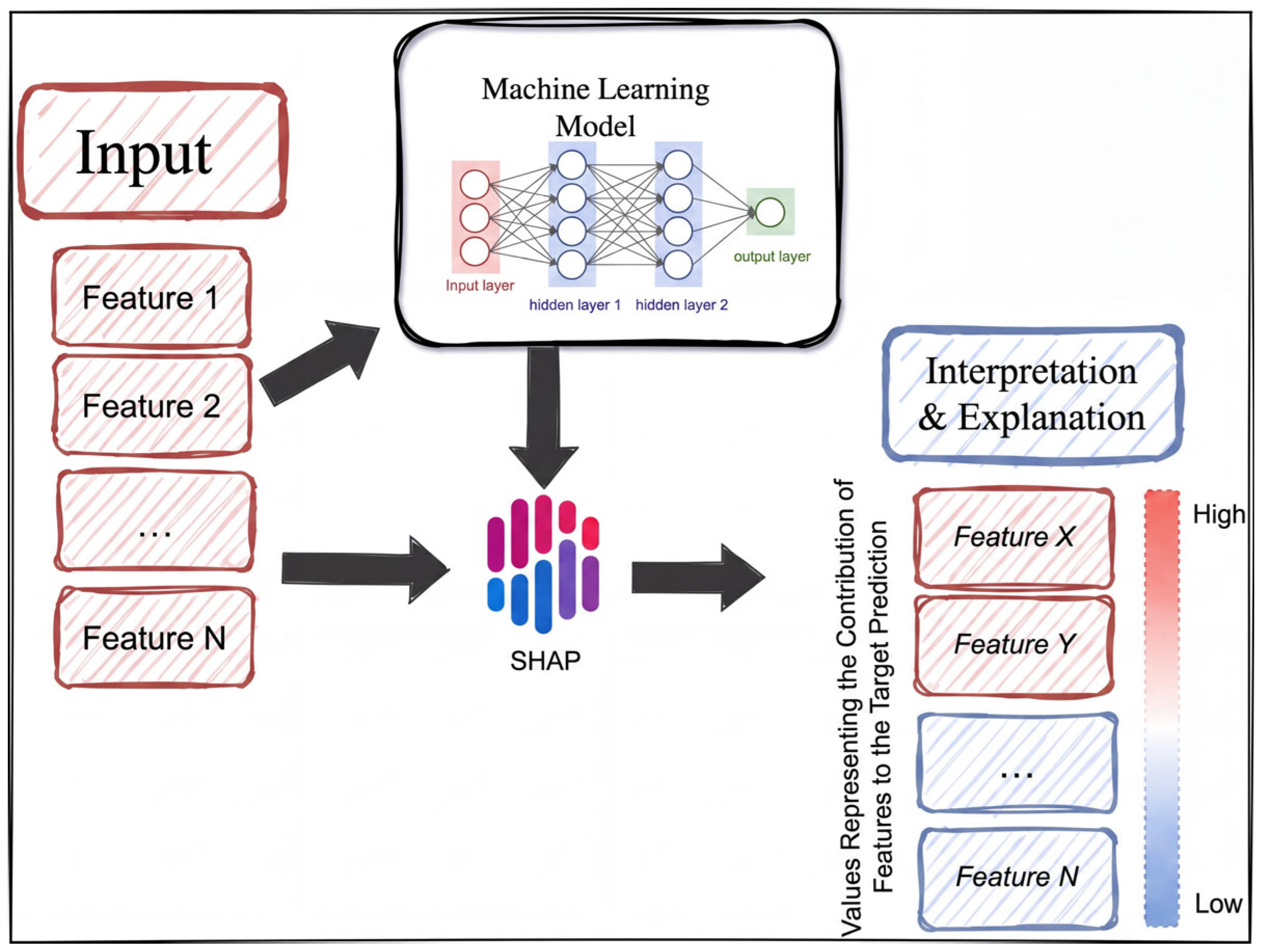
The SHAP (SHapley Additive exPlanations) method was used in this study to interpret the behavior of predictive models and understand how each groundwater quality parameter affects the IWQI (Figure 3). Based on game theory, SHAP assigns each feature a contribution value known as the Shapley value, which represents its average impact on the model’s output across all possible combinations of features [26,43,79,80,81]. The contribution of the variable using SHAP is given by:

$${\phi }_i={\sum }_{S\subseteq \mathrm{N}\left\{\mathrm{i}\right\}}^{N\ast }{\displaystyle \frac{\left|S\right|!\left(\left|N\right|-\left|S\right|-1\right)!}{\left|N\right|!}}|f\left(S\cup \left\{i\right\}\right)-f(S)|$$

(21)

where

• N: set of all features
• S: any subset of features not containing feature i
• f(S): model prediction when only feature in S are included
• f($S\cup \left\{i\right\}$): prediction when adding I to the subset
• ${\phi }_i$: contribution of feature i

Figure 3. Flowchart illustrating the SHAP value computation process for machine learning model interpretability.

Figure 3. Flowchart illustrating the SHAP value computation process for machine learning model interpretability.

Recent scientific literature reveals that SHAP has emerged as a widely used tool for interpreting machine learning models in environmental sciences. In the field of water quality, several studies have demonstrated its effectiveness, particularly for irrigation assessment and analysis of hydrochemical parameters. This method provides clear, quantifiable explanations of how each variable influences the model’s predictions. Its increasing use in environmental research underscores its importance for enhancing the clarity and explainability of complex models. Consequently, the application of SHAP in this study is fully justified for analyzing and understanding the determinants of irrigation water quality.

SHapley Additive ExPlanations decomposes each prediction into constituent components, thereby enabling the identification of hydrochemical variables that exert the most substantial influence on groundwater quality. This approach proves particularly valuable in water-scarce regions such as Djelfa Province, where informed decision-making is critical for sustainable water resource management. By quantitatively ranking features according to their actual contribution to model predictions, SHAP facilitates input optimization, enhances model interpretability and reliability assessment, and supports evidence-based water management strategies. The implementation of SHAP analysis in the present investigation delivers a solid, scientifically rigorous methodology for pinpointing the main factors affecting groundwater quality in Djelfa Province.

4. Results and Discussion

4.1. Statistical Summary of Physicochemical Parameters

The descriptive statistics presented in Table 1 reveal notable distribution characteristics and variability across all measured parameters. PH exhibits a slightly right-skewed distribution (skewness 0.75, kurtosis −0.41, mean 7.63 ± 0.45), confirming the near-neutral to slightly alkaline conditions observed across the study area. EC displays a moderately right-skewed distribution (skewness 0.90, kurtosis −0.31, and mean 1653.77 ± 910.45 µS/cm), reflecting spatial heterogeneity in groundwater mineralization. Among major cations, Ca²⁺ shows moderate positive skewness (1.48) and kurtosis (2.29), with a mean of 105.41 ± 68.61 mg/L, indicating isolated high concentration samples attributable to carbonate dissolution. Mg²⁺ exhibits exceptionally high skewness (6.05) and kurtosis (56.19), with a mean of 72.83 ± 64.04 mg/L, reflecting a strongly right-skewed distribution with pronounced extreme values consistent with localized dolomite dissolution. Na⁺ displays high positive skewness (3.41) and elevated kurtosis (16.58), with a mean of 128.76 ± 121.28 mg/L, suggesting spatially heterogeneous cation exchange processes and evaporative enrichment. K⁺ shows exceptionally high skewness (4.25) and kurtosis (21.49), with a mean of 7.85 ± 9.12 mg/L, indicating a strongly right-skewed distribution with extreme values likely attributable to localized fertilizer inputs. Among major anions, Cl⁻ exhibits positive skewness (2.90) and elevated kurtosis (13.17), with a mean of 256.65 ± 233.06 mg/L, reflecting evaporative salt accumulation and irrigation return flows. SO₄²⁻ shows high positive skewness (4.02) and pronounced kurtosis (24.81), with a mean of 271.36 ± 314.48 mg/L, indicating extreme outliers attributable to gypsum dissolution and agricultural inputs. HCO₃⁻ displays high skewness (4.88) and marked kurtosis (33.24), with a mean of 229.11 ± 141.99 mg/L, reflecting variable carbonate buffering capacity across the aquifer. In contrast, NO₃⁻ exhibits a near-symmetric distribution (skewness 0.74, kurtosis −0.48, mean 30.31 ± 21.46 mg/L), consistent with diffuse anthropogenic nitrogen inputs from agricultural activities. Finally, TH shows high positive skewness (3.28) and pronounced kurtosis (20.89), with a mean of 56.70 ± 37.93 °F, reflecting dominant Ca²⁺ and Mg²⁺ mineralization from carbonate and dolomite dissolution across the Ain Oussera Plain aquifer system.

4.2. Correlation Analysis and Hydrochemical Relationships

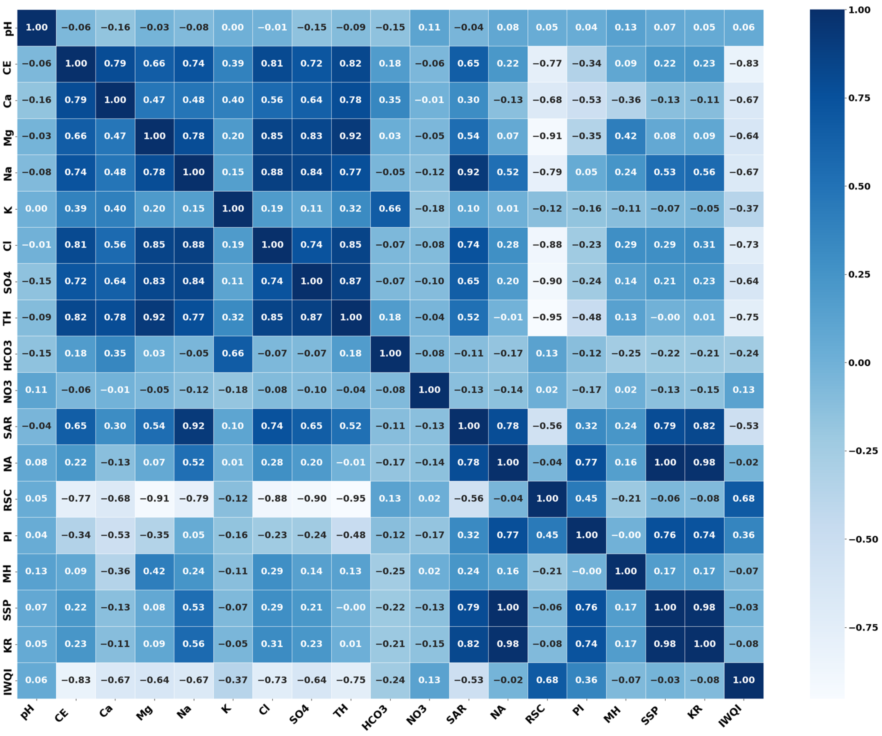
Pearson correlation matrix analysis (Figure 4) revealed substantial interdependencies among hydrochemical parameters, providing insights into geochemical processes and water-rock interactions within the aquifer system of the Ain Oussera plain. Electrical conductivity (EC) exhibited strong positive correlations (r > 0.8) with several ionic constituents, specifically chlorides (r = 0.81) and total hardness (r = 0.82), indicating that these parameters are primary contributors to overall water mineralization [82]. This relationship suggests progressive mineral dissolution along groundwater flow paths and potential anthropogenic contamination in certain zones, consistent with observations in similar semi-arid aquifer systems [83].

Significant intercorrelations were observed within the ionic system, particularly between magnesium and total hardness (r = 0.92), chlorides and magnesium (r = 0.85), and chlorides and sulfates (r = 0.83). These associations indicate familiar geochemical sources, likely the dissolution of evaporite minerals and carbonate rocks within the aquifer formation [84,85]. Similarly, strong correlations between sodium and both chlorides (r = 0.88) and sulfates (r = 0.84) suggest halite (NaCl) and gypsum (CaSO₄·2H₂O) dissolution processes, consistent with semi-arid hydrogeochemical environments where evaporation concentrates dissolved salts [38,86].

Potassium and calcium demonstrated intermediate correlations with bicarbonates (r = 0.66) and electrical conductivity (r = 0.79), respectively. In contrast, pH and nitrates showed minimal or slightly negative correlations with most parameters, indicating their relative independence from the primary mineralization processes. The weak correlation between pH and other parameters is consistent with carbonate buffering in the aquifer system. In contrast, nitrate variability likely reflects localized anthropogenic inputs from intensive agricultural practices and fertilizer application rather than natural geochemical processes [87].

Analysis of the correlation matrix reveals critical limiting factors for irrigation water quality, with electrical conductivity (EC) exhibiting the strongest negative correlation (−0.83) with IWQI, confirming that total salinity represents the primary limiting factor by creating saline stress conditions unfavorable to crop production. Total hardness (TH) (−0.75) and chlorides (−0.73) also demonstrate strong negative correlations, indicating that elevated concentrations of these parameters induce specific toxicity and contribute to soil salinization, whereas major cations Ca (−0.67), Na (−0.67), and Mg (−0.64) present moderate to strong negative correlations, underscoring their differential impact on irrigation water quality since, although essential for plant nutrition, they become problematic at high concentrations by affecting soil structure and ionic balance. In this context, the moderate negative correlation between SAR and IWQI (−0.53) indicates that an increase in the sodium adsorption ratio is associated with a decrease in the irrigation water quality index, which is consistent with fundamental principles of soil chemistry and agronomy. Specialized indices exhibit contrasting patterns: RSC (0.68) shows a moderate positive correlation, suggesting that appropriate residual sodium carbonate values contribute favorably to irrigation water quality. In contrast, the permeability index (PI) (0.36) confirms its positive role in maintaining soil permeability. Conversely, sulfates (−0.64) display a moderate negative correlation, indicating their contribution to salinization. Secondary parameters such as bicarbonates (−0.24) and nitrates (0.13) exhibit weak correlations, suggesting limited influence on the overall index, whereas pH (0.055) presents a negligible correlation with IWQI, indicating that this parameter is not determinant within the studied range, likely because values remain within acceptable limits for irrigation.

4.3. Irrigation Water Quality Index Assessments

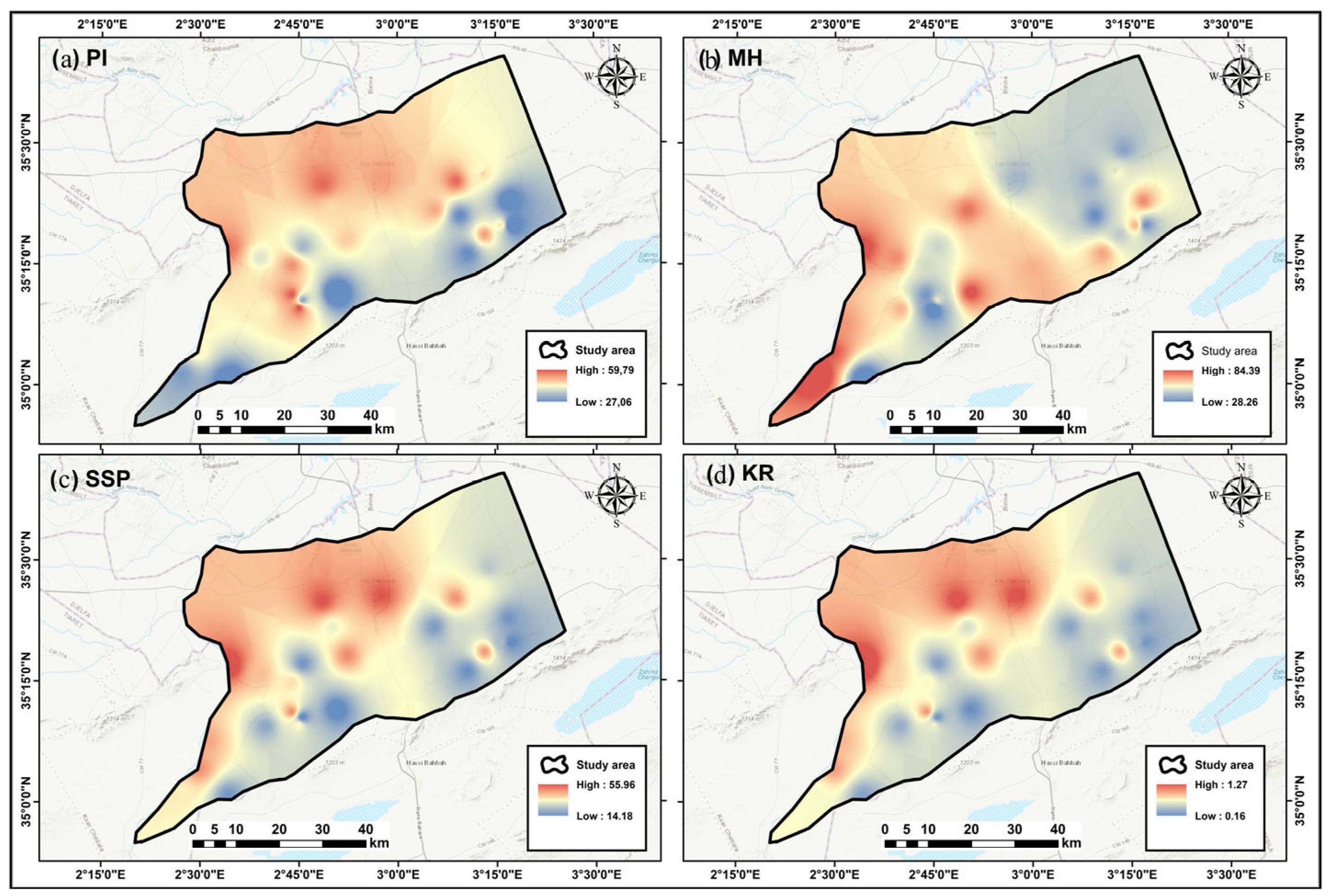
To comprehensively evaluate groundwater suitability for irrigation, multiple hydrochemical indices were calculated and assessed, including the sodium adsorption ratio (SAR), electrical conductivity (EC), sodium percentage (Na%), magnesium hazard (MH), Permeability Index (PI), soluble sodium percentage (SSP), Residual Sodium Carbonate (RSC), and Kelly’s ratio (KR). Descriptive statistics for groundwater quality indices are presented in

Table 5. Descriptive statistics of groundwater quality indices for irrigation.

Indices	Min	Max	Mean	Std Dev
EC	421.00	3800.00	1653.77	910.45
SAR	0.62	9.83	2.75	2.13
NA%	15.85	56.06	33.91	11.10
RSC	−67.40	−0.88	−9.94	12.46
PI	27.04	59.91	46.50	9.30
MH	28.09	84.41	55.89	13.88
SSP	14.16	55.96	32.84	11.73
KR	0.16	1.27	0.53	0.28
IWQI	29.60	96.04	65.47	16.25

(Figure 5). The multi-index methodology utilized within this research facilitates a thorough evaluation of agricultural water quality through examining multiple dimensions of soil-water-plant interactions, including salinity hazard, sodium hazard, permeability effects, and specific ion toxicity [2].

4.3.1. Electrical Conductivity (EC)

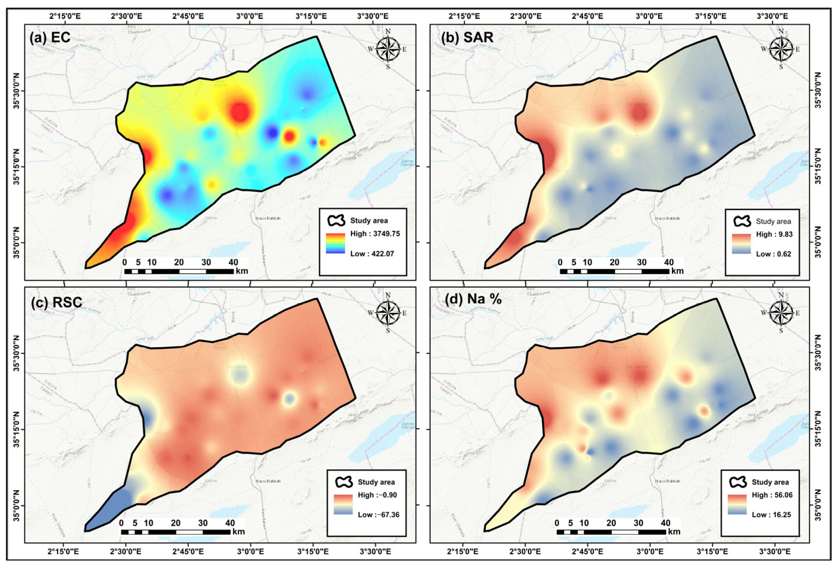
Electrical conductivity, representing total dissolved solids and overall salinity, ranged from 421 to 3800 µS/cm with a mean value of 1653.77 ± 910.45 µS/cm (Table 5). Wilcox (1955) [58] classified groundwater by electrical conductivity, indicating that samples from the Ain Oussera plain were grouped into three distinct categories. The majority of samples (68.59%) fall within the “Permissible” category (750–2250 µS/cm) for irrigation purposes, 23.56% of samples were classified as “Doubtful” (2250–5000 µS/cm) for irrigation suitability, and 7.85% demonstrated “Good” quality characteristics (250–750 µS/cm) for agricultural irrigation purposes according to

Table 6. Classification thresholds of groundwater quality indices for irrigation purposes.

Indices	Range	Water Quality	Number of Samples (%)	References
EC	<250 250–750 750–2250 2250–5000 >5000	Excellent Good Permissible Doubtful Unsuitable	0 (0%) 15 (7.85%) 131 (68.59%) 45 (23.56%) 0 (0%)	[58]
SAR	<10 10–18 18–26 >26	Excellent Good Doubtful Unsuitable	191 (100%) 0 (0%) 0 (0%) 0 (0%)	[57]
RSC	RSC < 1.25 1.25 > RSC < 2.5 RSC > 2.5	Good Medium Unsuitable	191 (100%) 0 (0%) 0 (0%)	[60]
Na%	<20% 20–40% 40–60% 60–80% >80%	Excellent Good Permissible Doubtful Unsuitable	28 (14.66%) 121 (63.65%) 42 (21.99%) 0 (0%) 0 (0%)	[58]
PI	>75% 25–75% <25%	Suitable Moderate Unsuitable	2 (1.05%) 182 (95.29%) 7 (3.66%)	[62]
MH	<50% >50%	Suitable Unsuitable	84 (43.98%) 107 (56.02%)	[59]
SSP	<50% >50%	Suitable Unsuitable	182 (95.29%) 9 (4.71%)	[61]
KR	<1 >1	Suitable Unsuitable	182 (95.29%) 9 (4.71%)	[63]
IWQI	85–100 70–85 55–70 40–55 0–40	No restriction Low restriction Moderate restriction High restriction Severe restriction	22 (11.52%) 83 (43.46%) 50 (26.18%) 29 (15.18%) 7 (3.66%)	[4]

. This salinity distribution reflects both natural mineral dissolution from the Albian sandstone aquifer formations and potential anthropogenic influences from intensive agricultural activities leading to elevated electrical conductivity [32]. The spatial distribution of EC reveals that higher salinity concentrations occur predominantly in areas with intensive agricultural practices, potentially related to longer groundwater residence times, reduced aquifer recharge, and cumulative evapotranspiration effects in semi-arid conditions.

4.3.2. Sodium Adsorption Ratio (SAR)

The Sodium Adsorption Ratio (SAR) serves as a critical parameter for evaluating sodium-related hazards in irrigation water, as it quantifies the alkali/sodium risk to crops [82,84]. This index explicitly indicates the propensity of irrigation water to participate in cation exchange reactions within the soil matrix. Water with SAR values exceeding 10 typically induces sodium accumulation in soils. According to the analytical results presented in Table 6, all water samples demonstrated excellent quality with respect to SAR, exhibiting values below 10. Figure 6b illustrates the spatial distribution of this index, clearly demonstrating that all sampled groundwater is suitable for irrigating agricultural areas. The low SAR values, combined with moderate salinity levels in the irrigation water, indicate negligible adverse effects on soil permeability and infiltration rates under appropriate irrigation management practices.

4.3.3. Sodium Percentage (Na%)

Sodium content is conventionally expressed as sodium percentage (Na %) or soluble sodium percentage. Evaluating irrigation water based on exchangeable sodium is essential, as sodium combined with carbonate or chloride can significantly compromise soil quality [2]. In the present study area, Na% concentrations ranged from 15.85% to 56.06%, with a mean value of 33.91 ± 11.10% (Table 5). According to the classification criteria presented in Table 6, sampled groundwater was categorized into three groups: 14.66% classified as “Excellent” (Na% < 20%), 63.65% as “Good” (20–40%), and 21.99% as “Permissible” (40–60%) for irrigation purposes based on [58] classification. No samples exceeded 60%, indicating that all groundwater is acceptable for irrigation use, though samples in the permissible category require appropriate soil management practices to prevent sodium accumulation.

4.3.4. Residual Sodium Carbonate (RSC)

The excess of carbonates and bicarbonates relative to calcium and magnesium concentrations in groundwater also influences irrigation suitability. This phenomenon, termed Residual Sodium Carbonate (RSC), was initially proposed by Eaton [60] and Richards [57] and is defined as the fraction of alkalinity not neutralized by divalent cations. This parameter is particularly relevant in evaluating the precipitation potential of calcite and magnesium carbonate minerals. RSC was calculated to assess the adverse effects of carbonate and bicarbonate concentrations on groundwater suitability for agricultural water use [60]. In this investigation, RSC values ranged from −67.40 to −0.88 meq/L, with a mean value of −9.94 ± 12.46 meq/L (Table 5). All samples in Table 6 (100%) exhibited negative RSC values, below 1.25 meq/L, and were classified as “Good” for irrigation according to Eaton [60] classification criteria. Negative RSC indicates that the sum of calcium and magnesium exceeds carbonates and bicarbonates, preventing precipitation of these divalent cations and subsequent sodium accumulation in soil solution.

4.3.5. Permeability Index (PI)

Soil permeability is adversely influenced by long-term irrigation water deployment and is regulated by sodium, calcium, magnesium, and bicarbonate concentrations throughout the soil system [59,62]. The Permeability Index (PI) of groundwater in the study area ranged from 27.04% to 59.91%, with a mean value of 46.50 ± 9.30% (Table 5). According to the PI classification criteria (Table 6), 95.29% of groundwater samples fall into Class II (25–75%), indicating moderate suitability for irrigation. Only 1.05% of samples exceeded 75% (Class I, “Suitable”), while 3.66% (seven sampling locations) fell below 25% (Class III, “Unsuitable”), classified as poor quality for irrigation purposes. The moderate PI values suggest that most groundwater maintains acceptable permeability characteristics. However, localized zones with low PI require enhanced drainage systems or calcium amendments to maintain adequate soil infiltration rates.

4.3.6. Magnesium Hazard (MH)

The magnesium hazard (MH) quantifies the effect of magnesium in irrigation water relative to calcium. Excessive magnesium concentrations adversely affect soil quality by increasing alkalinity and reducing calcium availability, ultimately impairing soil structure and reducing crop yields [59,86]. In the present investigation, MH values ranged from 28.09% to 84.41% (Figure 7b), with a mean of 55.89 ± 13.88%. The MH assessment results indicate that 43.98% of groundwater samples exhibited MH values below 50, classified as “Suitable”, rendering them suitable for irrigation according to Paliwali [88] criteria cited in Table 6. Conversely, 56.02% of samples showed MH values exceeding 50, indicating that these waters are unsuitable for irrigation. Elevated MH zones correspond with areas of high total hardness, suggesting progressive magnesium enrichment through dissolution of dolomitic limestone in the aquifer formation [32].

4.3.7. Soluble Sodium Percentage (SSP)

The Soluble Sodium Percentage (SSP) represents a critical parameter for evaluating irrigation water quality and long-term sodium accumulation risks. In the present study, SSP values ranged from 14.16% to 55.96% (Figure 7c), with a mean of 32.84 ± 11.73%. Notably, 95.29% of groundwater samples exhibited SSP values below 50, indicating “Suitable” water quality for irrigation applications according to the Todd [61] classification. Conversely, 4.71% of samples showed SSP values exceeding 50, indicating that these waters are unsuitable for irrigation. Waters with SSP above 50% pose increased risks of sodium-induced soil dispersion and reduced infiltration, particularly in soils with limited drainage or high clay content.

4.3.8. Kelly’s Ratio (KR)

Kelly’s Ratio (KR) constitutes one of the most significant parameters for categorizing water suitability for irrigation, representing the balance between sodium and alkaline earth metals (calcium and magnesium). A KR value exceeding 1 indicates excessive sodium concentration in the water. Kelly [63] recommended that this ratio for irrigation water should not surpass unity. In this investigation, KR values ranged from 0.16 to 1.27 (Figure 7d), with a mean of 0.53 ± 0.28. Approximately 95.29% of groundwater samples from the study area remained within the permissible limit (KR < 1) for irrigation water, indicating the absence of significant sodium excess in the examined groundwater resources. However, 4.71% of samples exceeded KR = 1, requiring targeted management interventions in areas with naturally poor drainage or fine-textured soils where sodium effects are exacerbated.

4.4. Irrigation Water Quality Index (IWQI) Assessment

The Irrigation Water Quality Index (IWQI) developed by [4] provides an integrated assessment of groundwater suitability for irrigation by synthesizing five critical parameters (EC, SAR, Na, Cl, HCO₃) into a single dimensionless score ranging from 0 to 100. IWQI values were calculated and evaluated according to five restriction categories presented in Table 6. When the calculated index value exceeds 55, the area is considered to experience minimal constraints regarding irrigation water quality. Consequently, a well drilled within such an area can be regarded as suitable for irrigation purposes.

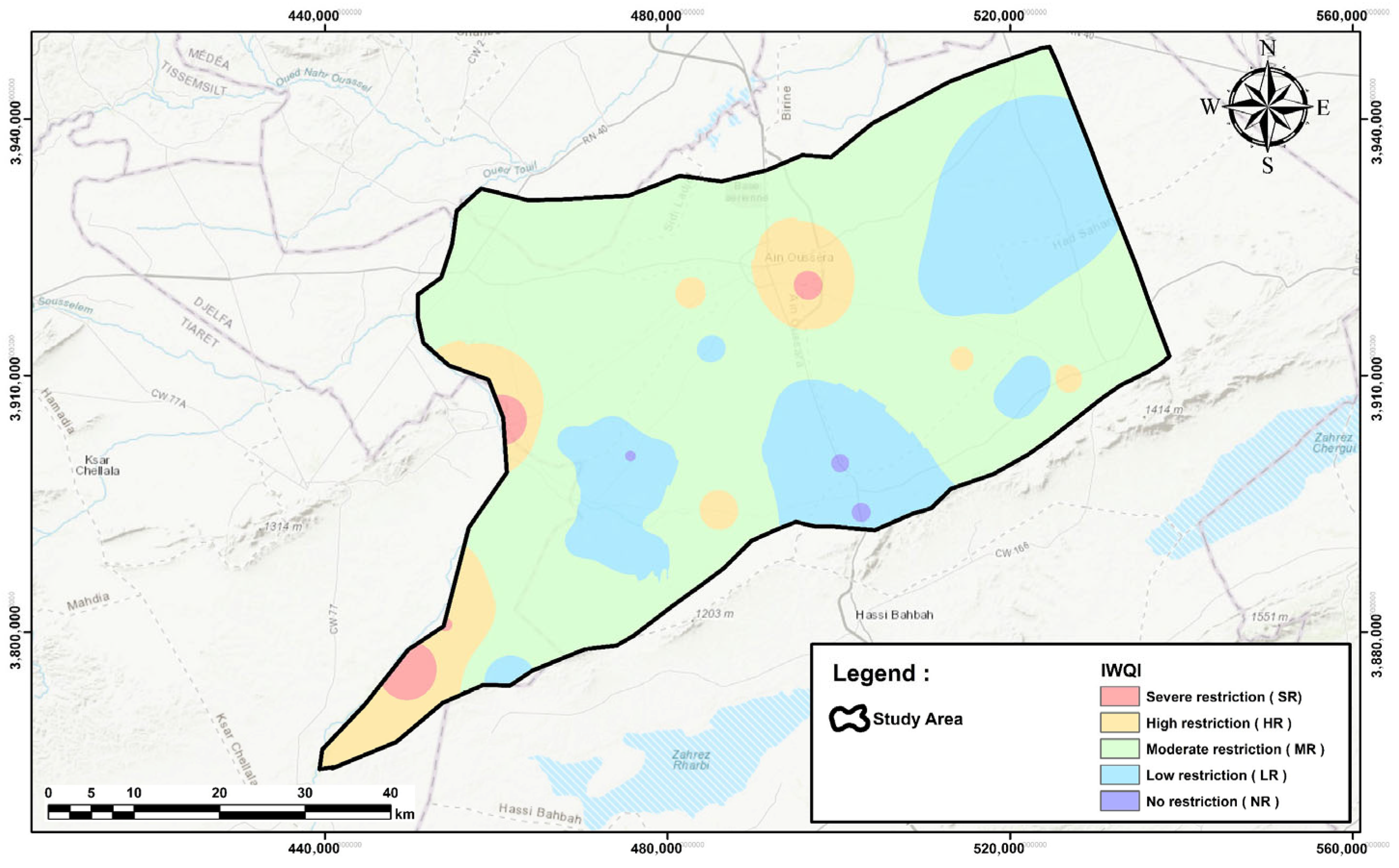
In the study area, IWQI values ranged from 29.60 to 96.04 (Table 5), with a mean value of 65.47 ± 16.25. Approximately 3.66% of the samples (7 samples) were classified as “Severe Restriction” (SR, IWQI 0–40) for irrigation use, indicating that groundwater in these zones can only be used for highly salt-tolerant crops with adequate leaching and drainage provisions. About 15.18% of samples (29 samples) fell into the “High Restriction” (HR, IWQI 40–55) category, suggesting considerable potential for soil damage that could compromise plant health and ultimately lead to crop failure. To mitigate these effects, salt leaching practices are imperative in such areas. Moreover, 26.18% of the samples (50 samples) were classified under “Moderate Restriction” (MR, IWQI 55–70); these waters are suitable for use in soils with moderate to high permeability, where moderate salt leaching can be practiced, and moderately salt-tolerant crops may be cultivated. A further 43.46% of the samples (83) were categorized as “Low Restriction” (LR, IWQI 70–85), recommended for application in irrigated soils with light texture or moderate permeability, particularly for salt leaching. However, sodicity problems may develop in heavy-textured soils, and its application in clay-rich soils is discouraged. Finally, 11.52% of the study area (22 samples) was classified as “No Restriction” (NR, IWQI 85–100), indicating suitability for most soil types with a low probability of inducing salinity or sodicity issues (Table 6; Figure 8).

IWQI values below 55 (representing 18.84% of samples) correspond to groundwater from regions such as Ain Oussera city, Oued Touil, and the Guernini commune, which should be used cautiously or avoided altogether, especially for salt-sensitive crops when better-quality alternatives are available. The deterioration in irrigation water quality in these locations is likely attributable to anthropogenic influences, including the discharge of urban wastewater and the excessive use of chemical fertilizers in agricultural lands [32]. This spatial distribution pattern is consistent with findings from other semi-arid Algerian regions where intensive agricultural activities and inadequate wastewater management have contributed to groundwater quality degradation [42,43].

4.5. Machine Learning Algorithm Construction and Hyperparameter Tuning

Five algorithms were developed for IWQI prediction. Each algorithm was subjected to rigorous hyperparameter optimization via a grid search, in which all possible combinations of predefined hyperparameter values were explored to identify the configuration yielding optimal predictive performance. For each hyperparameter combination, model performance was evaluated using 5-fold cross-validation, with averaged metrics across folds serving as the final performance indicators to ensure robust, generalizable results. The dataset was partitioned into training (80%) and test (20%) subsets, with the training data further split for cross-validation within each fold to maintain data independence and mitigate overfitting. Hyperparameter configurations that yielded the highest coefficient of determination (R²) during the grid search were selected as optimal. Multiple performance metrics were systematically computed, including R², Root Mean Squared Error (RMSE), and Mean Absolute Error (MAE), whose values served as the quantitative assessment of model efficacy. The optimized hyperparameters for each algorithm are presented in

Table 7. Hyperparameter tuning for selected models.

Model	Optimized Hyperparameters
Support Vector Regression (SVR)	C = 100 Epsilon = 0.2 Gamma = auto Kernel = rbf
Random Forest Regressor	max_depth = 20 max_features = sqrt min_samples_leaf = 1 min_samples_split = 5 n_estimators = 200
Gradient Boosting Regressor	learning_rate = 0.1 max_depth = 3 min_samples_split = 5 n_estimators = 100 subsample = 0.8
XGBoost Regressor	colsample_bytree = 0.7 learning_rate = 0.1 max_depth = 3 n_estimators = 100 reg_alpha = 0.1 reg_lambda = 0.1 subsample = 0.9
K-Nearest Neighbors (KNN)	algorithm = auto n_neighbors = 7 p = 1 (Manhattan distance) weights = distance

. This cross-validated optimization pipeline ensured equitable performance estimation across diverse algorithmic architectures and facilitated unbiased comparative evaluation among competing models, thereby enabling the identification of the most suitable regression framework for IWQI prediction.

XGBoost calibration targeted learning rate, maximum tree depth, number of estimators, subsample ratio, and column sampling rate, harmonizing model intricacy with generalization ability [15]. Random Forest optimization addressed the number of trees, the maximum number of features per split, and the minimum number of samples per leaf, resulting in robust ensemble predictions [13]. Gradient Boosting hyperparameter tuning targeted learning rate, tree depth, and boosting iterations, achieving an optimal balance between training efficiency and prediction accuracy [14]. For SVR, the regularization parameter (C), epsilon-tube width, and kernel coefficient (gamma) were systematically optimized [73]. K-Nearest Neighbors optimization determined the optimal number of neighbors (k) and distance metric.

4.6. Feature Selection and Variable Importance

A comprehensive feature selection pipeline was implemented to identify the optimal water quality parameters for predicting the Irrigation Water Quality Index (IWQI). This integrated approach combined Recursive Feature Elimination with Cross-Validation (RFECV), correlation analysis, and hydrogeochemical domain knowledge to systematically reduce the initial set of 18 water quality parameters (pH, EC, Ca²⁺, Mg²⁺, Na⁺, K⁺, Cl⁻, SO₄²⁻, HCO₃⁻, NO₃⁻, TH, SAR, RSC, MH, PI, KR, SSP, Na%) to the most influential predictors. The RFECV technique was applied using five-fold cross-validation, in which the least contributing variable was iteratively removed during model training to maximize the cross-validated R² score. The optimization curve showed that cross-validated R² scores increased substantially with the inclusion of additional predictors, achieving maximum performance with six features, beyond which marginal gains plateaued or even declined slightly (Figure 9) The RFECV stopping criterion, selecting 6 features at the point where additional predictors produced no meaningful improvement in cross-validated R², is further supported by hydrogeochemical reasoning: the six selected parameters (EC, Na⁺, Cl⁻, SAR, TH, Mg²⁺) collectively represent all four principal quality dimensions of the IWQI formula, salinity, sodicity, specific ion toxicity, and hardness, ensuring that the reduced feature set retains full hydrochemical representativeness. Min-max normalisation was chosen over z-score standardisation because the IWQI prediction task requires bounded input ranges that preserve the relative magnitude relationships between hydrochemical parameters, which z-score normalisation would distort through mean-centering [9]. This inflection point represented the optimal balance between model complexity and predictive accuracy.

Following RFECV analysis and considering correlation coefficients with IWQI from the Pearson correlation matrix (Figure 4) and practical relevance based on domain expertise in irrigation water quality, six parameters were selected as optimal inputs: electrical conductivity (EC), sodium (Na⁺), chloride (Cl⁻), sodium adsorption ratio (SAR), total hardness (TH), and magnesium (Mg²⁺). These variables constitute the fundamental ionic determinants governing irrigation water suitability, consistent with the parameters that showed the strongest negative correlations with IWQI in the statistical analysis (Section 4.2). The integration of multiple feature selection techniques ensured that selected features aligned with both statistical and hydrogeochemical significance, addressing limitations inherent to individual approaches and yielding a more robust and interpretable predictive model for sustainable water resource management.

4.7. Machine Learning Model Performance and Comparative Evaluation

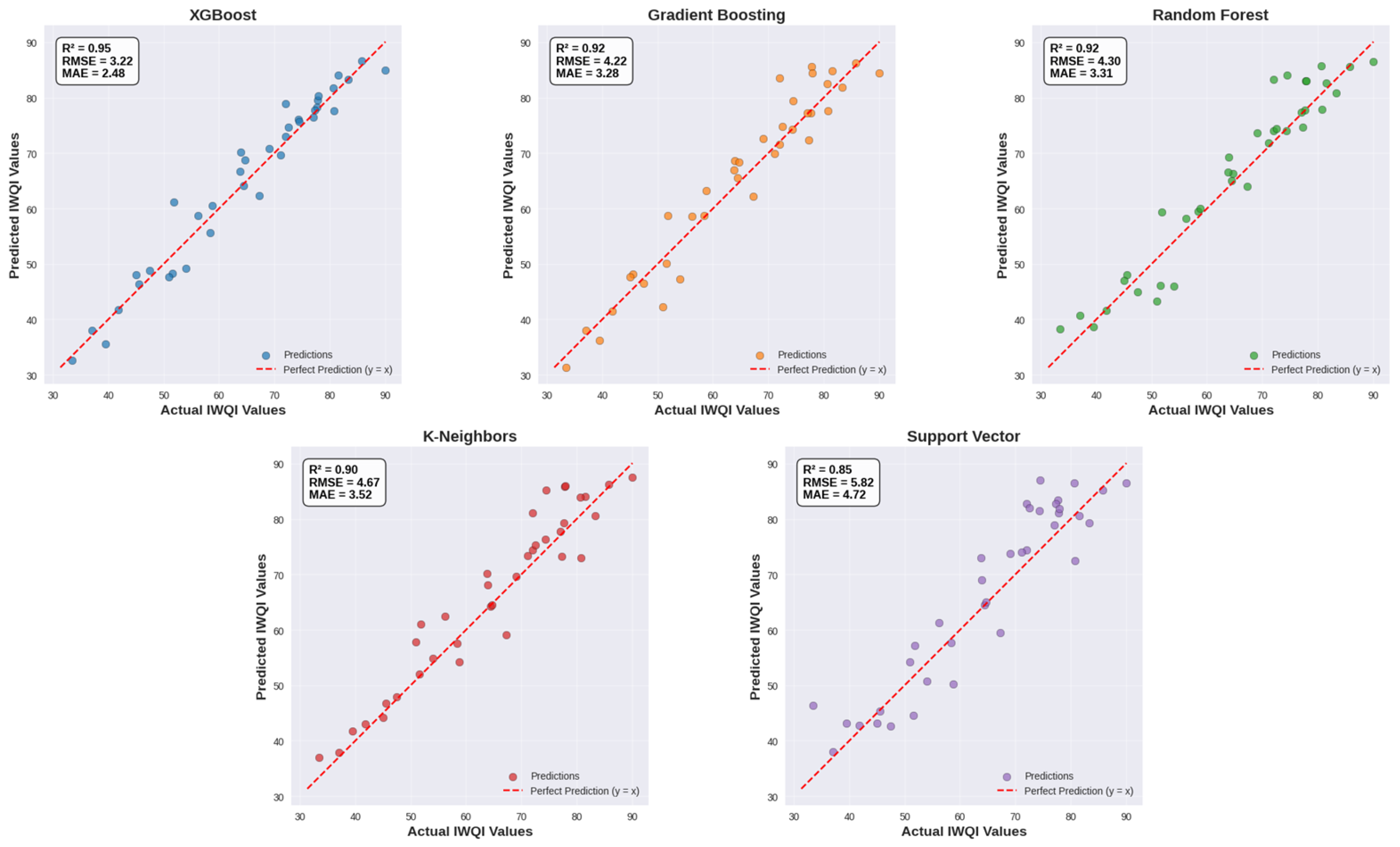
The comparative evaluation of machine learning regression algorithms showed substantial variation in predictive accuracy across the five examined models, as measured using multiple statistical indicators: the coefficient of determination (R²), root mean squared error (RMSE), and mean absolute error (MAE) on the testing subset. The XGBoost algorithm emerged as the superior predictive framework, achieving an exceptional R² value of 0.95 ± 0.03, accompanied by minimal prediction errors characterized by an RMSE of 3.22 ± 0.30 and MAE of 2.48 ± 0.36, thereby demonstrating its capacity to capture 95% of IWQI variance while maintaining remarkably low deviation magnitudes consistent with findings from other Algerian groundwater studies [42,43]. The Gradient Boosting algorithm secured the second-highest performance tier, attaining an R² of 0.92 ± 0.05 with corresponding RMSE and MAE values of 4.22 ± 0.44 and 3.28 ± 0.36, respectively, indicating robust predictive capability with only a marginal reduction relative to the optimal model. The Random Forest algorithm exhibited comparable efficacy, yielding an R² of 0.92 ± 0.04, an RMSE of 4.30 ± 0.51, and an MAE of 3.31 ± 0.48, thereby positioning it within the high-performing ensemble algorithms.

The K-Nearest Neighbors (KNN) algorithm demonstrated moderately strong performance, achieving an R² of 0.90 ± 0.03, an RMSE of 4.67 ± 0.66, and an MAE of 3.52 ± 0.52. While the Support Vector Regressor (SVR) achieved an R² of 0.85 ± 0.02, along with elevated error metrics (RMSE = 5.82 ± 0.92, MAE = 4.72 ± 0.59), indicating diminished predictive precision compared to ensemble methods.

The superior performance of tree-based ensemble methods, particularly XGBoosting, Random Forests, and Gradient Boosting, can be attributed to their ability to capture non-linear relationships and complex interactions among hydrochemical parameters through hierarchical decision tree structures and boosting/bagging mechanisms [13,14,15]. In contrast. Cross-validation results confirmed model stability across different data partitions, with XGBoost, Random Forest, and Gradient Boosting maintaining consistent performance across validation folds, demonstrating robust generalization capability. These performance hierarchies, comprehensively illustrated in Figure 10, demonstrate that tree-based ensemble methods, particularly XGBoost and Gradient Boosting, are optimally suited for IWQI prediction in the Ain Oussera plain.

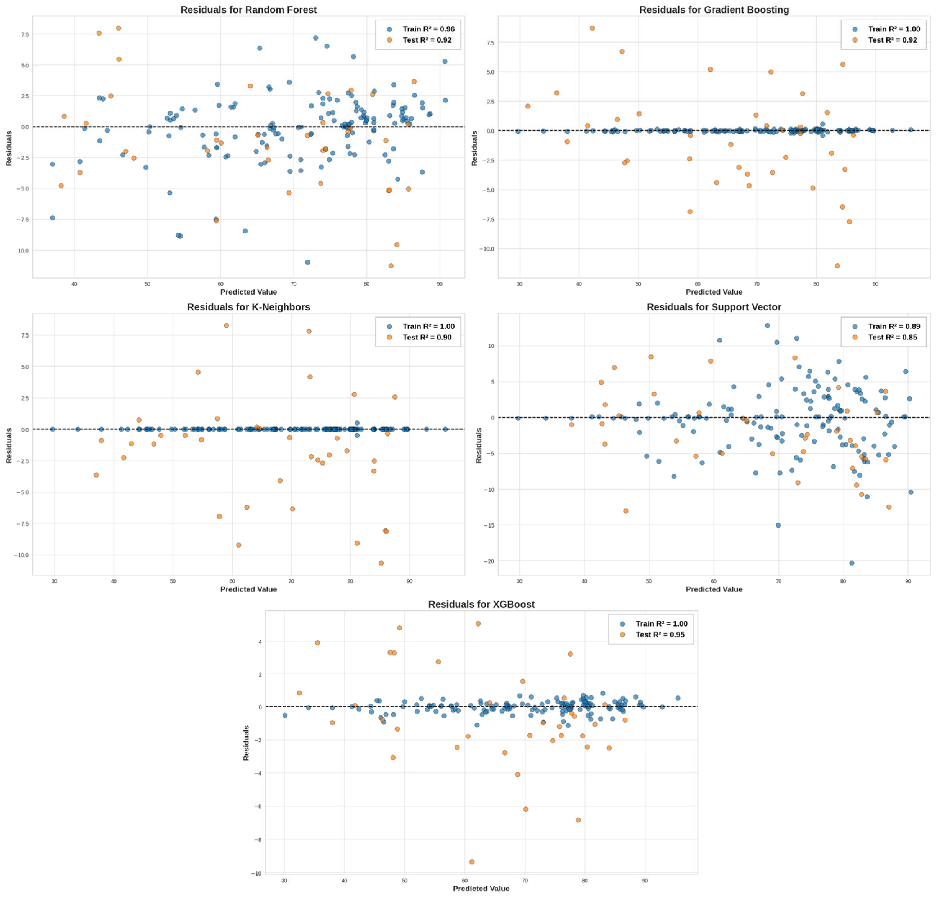
Figure 11 presents the residual distribution patterns for all five machine learning models, revealing substantial inter-model variability in prediction error characteristics and model fit quality. Support Vector Regression exhibits wider, more dispersed residual distributions, indicating elevated prediction errors and diminished capacity to capture the complex, nonlinear hydrochemical relationships governing IWQI variability. Conversely, tree-based ensemble models, including Random Forest, Gradient Boosting, and XGBoost, alongside the K-Nearest Neighbors algorithm, demonstrate markedly tighter clustering of residuals near zero, thereby reflecting superior predictive accuracy and enhanced model fidelity. In contrast, XGBoost residuals exhibit near-random distribution around zero with minimal systematic bias, validating its appropriateness for IWQI prediction in the Ain Oussera plain.

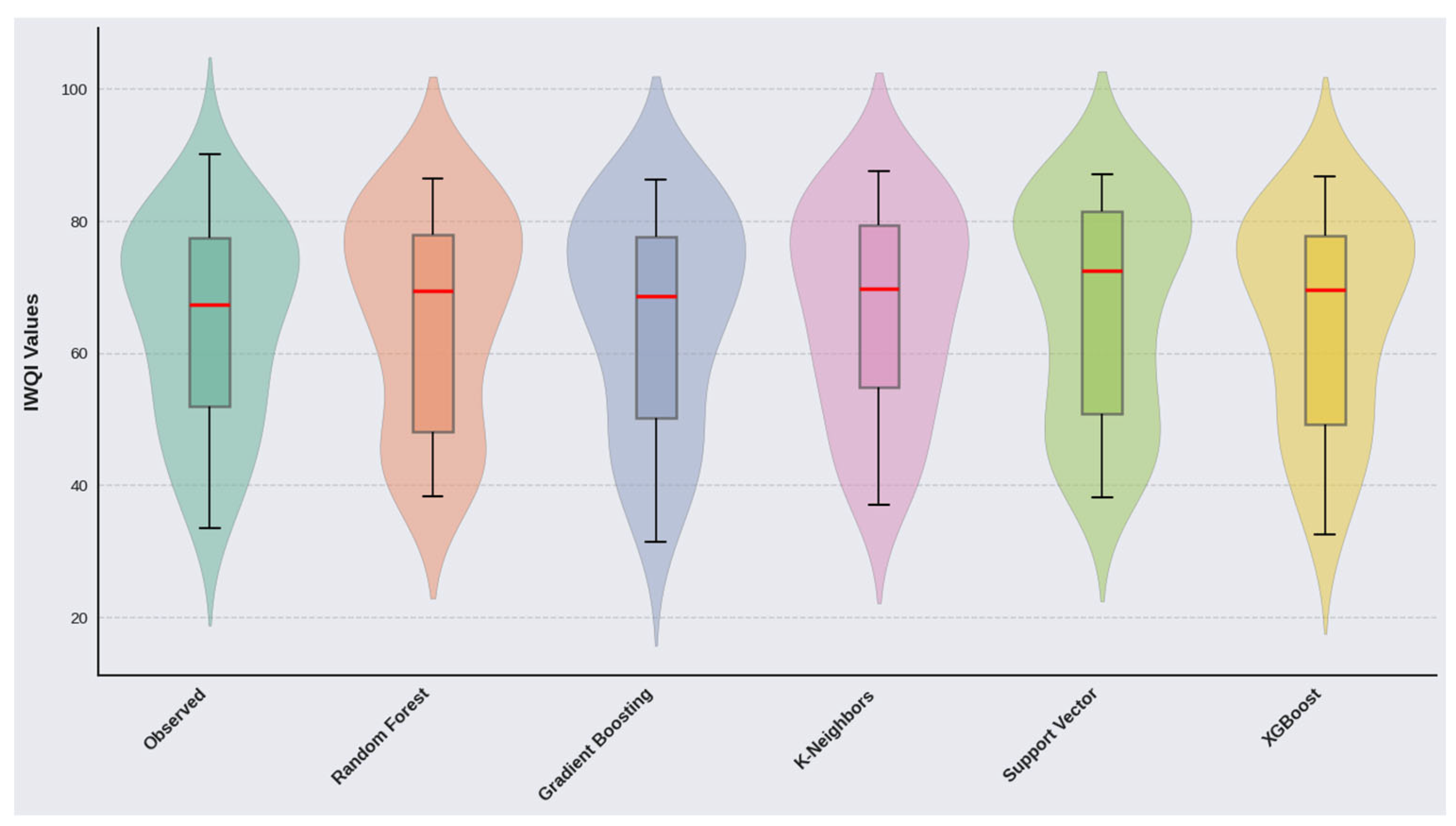
The violin box and whisker plot in Figure 12 shows that all machine learning models reproduce the distributional characteristics of the observed IWQI values. The majority of values are concentrated in the 55–75 intervals, and the median is near 68. All predicted distributions fall within comparable ranges, indicating that each algorithm captures the overall patterns of the irrigation water quality index. Random Forest produces a narrower, more stable distribution, ranging from approximately 39 to 88, with a median around 72, reflecting enhanced predictive consistency and reduced outliers. Gradient Boosting and XGBoost similarly demonstrate compact and well-controlled distributions, spanning approximately 36 to 88 and with median values between 70 and 71, thereby evidencing consistent and precise predictions with minimal outlier generation. K-Nearest Neighbors displays a slightly wider distribution yet remains closely aligned with the observed pattern, with values predominantly concentrated between 65 and 78. Support Vector Regression likewise produces stable predictions, with most values ranging from 66 to 80 and a median near 70.

Ensemble techniques, specifically XGBoost, Random Forest, and Gradient Boosting, exhibit the most concentrated and stable predictive distributions, characterized by reduced variance and minimal extreme value generation compared to SVR [13,14,15]. This distributional coherence underscores the capacity of tree-based ensemble methods to maintain robust central tendency estimates while effectively constraining prediction uncertainty across the full spectrum of hydrochemical conditions encountered within the Ain Oussera Plain, consistent with findings from other semi-arid Algerian groundwater studies [42,43]

4.8. Model Interpretability via SHAP Analysis

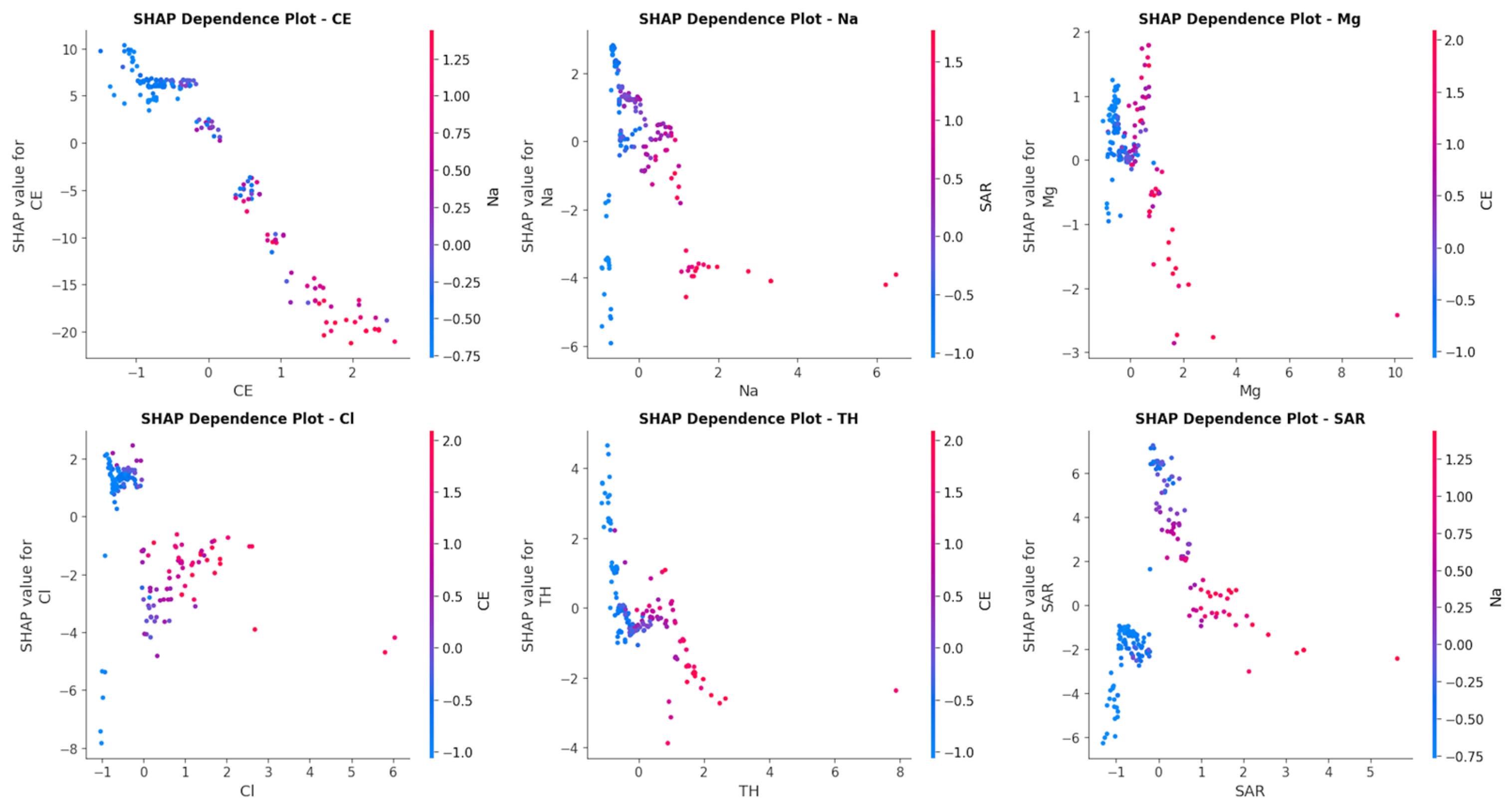
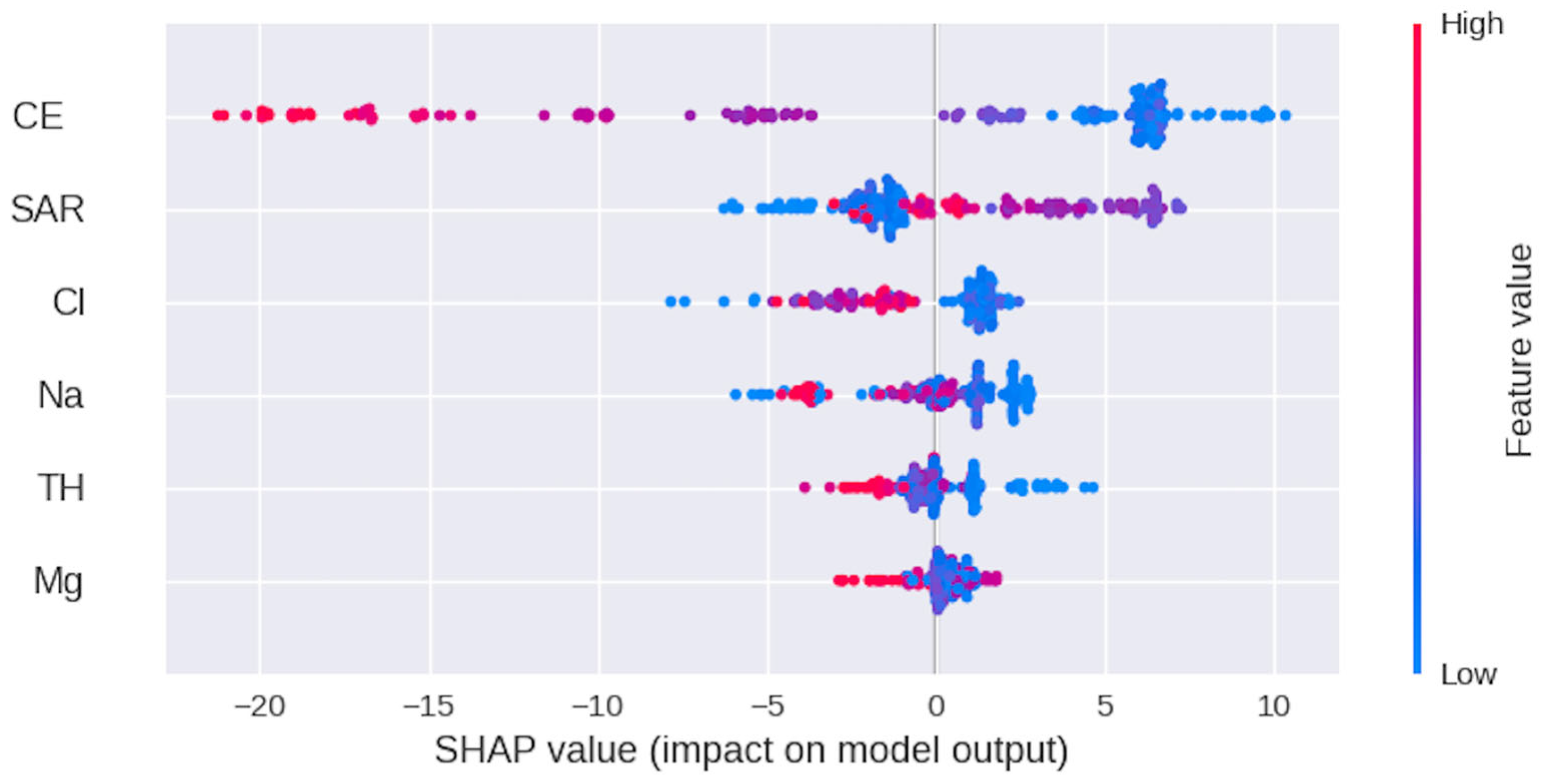
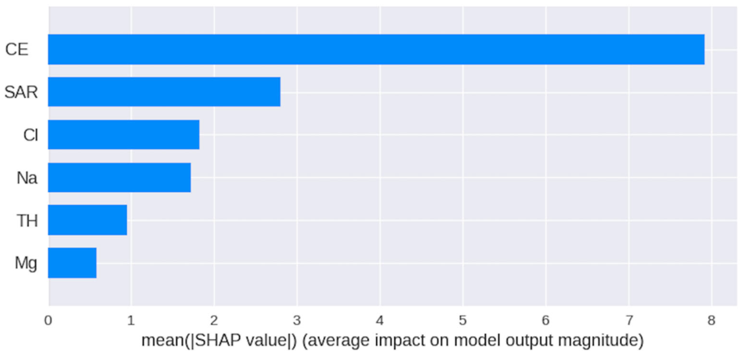
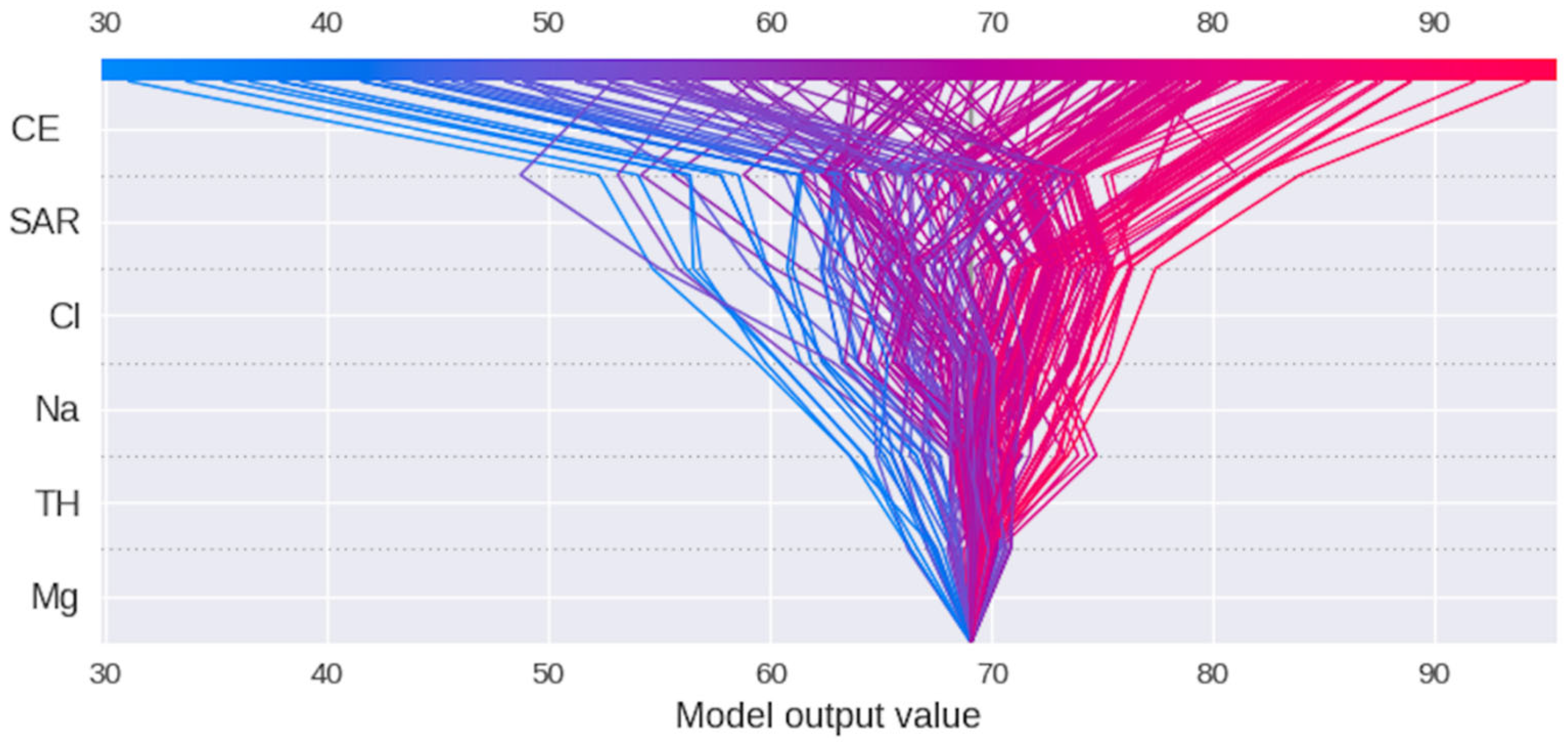
To enhance model transparency and elucidate the hydrochemical drivers underlying XGBoost predictions, SHAP (Shapley Additive exPlanations) analysis was implemented as a rigorous, model-agnostic interpretability framework developed by [26]. This game theoretic approach quantifies the marginal contribution of each hydrochemical parameter to individual predictions by computing Shapley values, which represent the average impact of a feature across all possible feature combinations. Figure 13 presents a comprehensive beeswarm plot visualizing the distribution of SHAP values for all six selected predictors, wherein each data point corresponds to an individual groundwater sample, the horizontal position conveys the extent and directionality of feature impact on model responses, and the color gradient portrays feature extent from low (blue) to high (red). Correspondingly, Figure 14 presents a horizontal bar chart categorizing variables by their mean absolute SHAP values, thereby providing a quantitative prioritization of feature weights based on average contribution across the whole dataset. Collectively, these visualizations facilitate both instance-level interpretation of individual predictions and a global understanding of aggregate feature influence patterns within the predictive framework.

Critically, the SHAP results are not interpreted in isolation but are systematically grounded in the hydrogeochemical processes identified through correlation analysis and multi-index assessment. This integration constitutes the scientific core of the study’s contribution and is elaborated below for each dominant feature. The SHAP beeswarm plot Figure 13 elucidates the magnitudes, directions, and distributions of individual feature contributions to IWQI predictions across all groundwater samples. Electrical conductivity (EC) exhibits the most pronounced SHAP value dispersion, spanning approximately −22 to +11, thereby constituting the dominant predictive driver with the widest individual impact range among all hydrochemical parameters. Critically, elevated EC concentrations (depicted in red) predominantly cluster in the strongly negative SHAP domain (−22 to −5), indicating that high salinity conditions systematically reduce predicted IWQI scores toward lower irrigation water quality classifications consistent with the strong negative correlation (r = −0.83) observed in Section 4.2. Conversely, low EC values (blue points) cluster in the positive SHAP region (+5 to +11), indicating that reduced salinity improves IWQI predictions by elevating them toward favorable quality thresholds. This bidirectional pattern validates EC as the primary determinant of IWQI spatial heterogeneity, reflecting the fundamental role of excessive total dissolved solids in constraining irrigation water suitability, while moderate salinity levels support acceptable agricultural applications within the Ain Oussera Plain.

The sodium adsorption ratio (SAR) emerges as the second most influential predictor, displaying SHAP values distributed predominantly between −6 and +6 with moderate dispersion. High SAR concentrations (red-purple points) are primarily concentrated in the negative SHAP domain (−6 to 0), indicating that elevated sodium relative to calcium and magnesium consistently decreases IWQI predictions and intensifies soil sodification hazards, including clay dispersion, reduced infiltration capacity, and structural degradation. Low SAR values (blue points) generate corresponding positive SHAP contributions (0 to +6), thereby improving predicted water quality classifications, aligning with the moderate negative correlation (r = −0.53) between SAR and IWQI observed in correlation analysis

Chloride (Cl⁻) and sodium (Na⁺) exhibit comparable moderate influence patterns, with SHAP values ranging from approximately −5 to +3 for chloride and from −4 to +4 for sodium. Both parameters exhibit negative SHAP contributions when present at elevated concentrations (red points clustering between −5 and 0), reflecting their deleterious effects on crop salt tolerance and specific ion toxicity that reduce irrigation water suitability, consistent with their strong negative correlations with IWQI (r = −0.73 for Cl⁻ and r = −0.67 for Na⁺). Total hardness (TH) and magnesium (Mg²⁺) display markedly constrained SHAP value distributions tightly clustered near zero, with TH spanning approximately −3 to +3 and Mg confined to −2 to +2. This narrow dispersion indicates limited individual impact on model predictions, suggesting that while these parameters contribute to overall hydrochemical characterization and were retained through RFECV optimization, their marginal effects on IWQI variability remain comparatively modest relative to salinity and sodicity indicators. These findings align with the moderate negative correlations observed for TH (r = −0.75) and Mg²⁺ (r = −0.64), where their influence on IWQI is present but secondary to EC, Na⁺, and Cl⁻.

The mean absolute SHAP value ranking in Figure 14 provides a complementary global perspective on feature importance by aggregating individual contributions across all predictions. Electrical conductivity (EC) as the dominant SHAP driver (mean SHAP = 7.91) directly reflects the primary hydrogeochemical process operating in the Ain Oussera Plain: the progressive dissolution of evaporite minerals, principally halite (NaCl) and gypsum (CaSO₄, 2H₂O), along groundwater flow paths from recharge zones toward the centre of the plain. This process, already evidenced by the strong positive correlations between EC and both Cl⁻ (r = 0.81) and TH (r = 0.82) identified in Section 4.2, is amplified in the semi-arid context where high evapotranspiration rates concentrate dissolved salts in shallow groundwater [38]. The sodium adsorption ratio ranks second, with a mean SHAP value of approximately 2.80, thereby establishing SAR as a critical secondary control on IWQI predictions and validating the fundamental role of sodification hazards in irrigation water evaluation frameworks. Chloride (Cl⁻, mean SHAP = 1.83) and sodium (Na⁺, mean SHAP = 1.73) exhibit comparable intermediate importance, consistent with their strong negative correlations with IWQI (r = −0.73 and r = −0.67, respectively). Their co-dominance in SHAP analysis confirms that Cl⁻ and Na⁺ act as geochemical tracers of the same mineralization process, halite dissolution, rather than independent stressors. This finding has a direct practical implication: monitoring programs can use EC as a proxy for the combined Cl⁻/Na⁺ hazard, reducing analytical costs without loss of diagnostic power, a conclusion consistent with the RFECV feature selection results, where EC alone explained the largest variance increment in model performance. Total hardness (TH, mean SHAP = 0.95) and magnesium (Mg²⁺, mean SHAP = 0.60) show comparatively modest SHAP contributions despite their moderate negative correlations with IWQI (r = −0.75 and r = −0.64, respectively). This apparent discrepancy is explained by the SHAP TH dependence plot, which reveals a bidirectional influence: moderate hardness exerts a protective buffering effect against sodium-induced soil dispersion by maintaining Ca²⁺ availability, while excessive hardness contributes to overall salinity burden. The net effect on IWQI is therefore non-monotonic, reducing the mean absolute SHAP contribution even though TH is mechanistically important. This nuance, invisible to standard correlation analysis, exemplifies why SHAP dependence plots provide hydrochemically richer insights than correlation coefficients alone.

Figure 15 presents a SHAP decision plot that illustrates the sequential, cumulative contribution of individual hydrochemical features to final IWQI predictions across all groundwater observations. This visualization depicts the decision-making pathway of the XGBoost model by tracking how predictions evolve from a baseline expected value through successive incorporation of feature contributions, with each trajectory line representing an individual sample’s progression toward its final predicted value. Features are arranged vertically in descending order of importance (EC, SAR, Cl, Na, TH, and Mg), with the horizontal axis denoting the cumulative SHAP values that determine the model output. This analytical framework facilitates a comprehensive interpretation of how specific feature combinations drive predictions across the full spectrum of observed water quality conditions and elucidates the hierarchical logic governing model decision-making processes.

The decision plot exhibits a distinctive convergence pattern wherein the majority of prediction trajectories coalesce around a final model output value of approximately 70, with a concentration zone extending from approximately 55 to 75, corresponding to the “Low Restriction” to “Moderate Restriction” IWQI categories. This convergence behavior indicates that, despite substantial heterogeneity in individual hydrochemical parameter values across the study aquifer, the XGBoost model generates predictions clustered within a relatively constrained range centered near the moderate irrigation water quality threshold, reflecting the predominantly moderate salinity conditions in the Ain Oussera Plain. The funnel-shaped trajectory pattern, characterized by progressive narrowing from the baseline value toward the final prediction zone, demonstrates that cumulative feature contributions tend toward central tendency stabilization rather than producing extreme outlier predictions. Nevertheless, a notable subset of trajectories diverges toward both lower (blue lines converging around 35–50) and higher (pink lines extending to 80–95) IWQI values, reflecting the model’s capacity to differentiate hydrochemically distinct water types while maintaining overall prediction stability. This distributional consistency closely matches the observed IWQI traits in Table 6 and validates the algorithm’s ability to capture the inherent variation within the groundwater quality evaluation system.

Figure 16 presents a comprehensive matrix of SHAP dependence plots that elucidate both univariate relationships between water quality parameters and their corresponding SHAP values, as well as bivariate interaction effects in which secondary features modulate the marginal impacts of primary predictors on IWQI predictions. Each subplot displays a primary feature along the horizontal axis, its associated SHAP value along the vertical axis, and point coloration encoding the magnitude of interacting secondary features, thereby facilitating simultaneous visualization of main effects and interaction dynamics across six parameters: electrical conductivity, sodium, magnesium, chloride, total hardness, and sodium adsorption ratio.

The EC dependence plot exhibits pronounced nonlinearity, with SHAP values transitioning from strongly positive (+10) at low EC concentrations to markedly negative (−20) at elevated EC levels, while Na interaction coloration reveals that elevated sodium concentrations (pink points) cluster predominantly within the negative SHAP domain at high EC values, signifying synergistic amplification of water quality degradation where combined salinity and sodium hazards exceed acceptable thresholds for irrigation. The SAR dependence plot demonstrates the most systematic and coherent relationship, spanning 12 SHAP units from +6 at minimal SAR to −6 at elevated SAR, with Na stratification indicating that high-sodium samples (pink) concentrate exclusively within the high-SAR negative SHAP domain, reflecting advanced sodification processes. In contrast, low-sodium samples (blue) occupy the low-SAR, positive SHAP region characteristic of favorable calcium-magnesium-dominated waters.

The TH plot reveals complex bidirectional influences (ranging from +5 to −4 SHAP units), in which moderate hardness provides protective buffering against sodium-induced hazards. In contrast, excessive hardness contributes to the overall salinity burden. The Cl plot shows that chloride’s predictive significance increases in high-salinity contexts (pink points exhibit the most pronounced negative SHAP contributions at elevated Cl concentrations). The Mg and Na dependence plots show similar patterns, with elevated concentrations driving negative SHAP values, though with smaller effect sizes than for EC and SAR. Collectively, the dependence plots substantiate that the XGBoost model successfully captures essential hydrochemical interaction mechanisms wherein EC and SAR emerge as predominant controls, their impacts amplified through synergistic associations with sodium and chloride, thereby revealing that water quality degradation emanates from specific configurations wherein multiple salinity-related stressors converge rather than from isolated parameter elevations a pattern consistent with hydrogeochemical processes in semi-arid aquifer systems [32,38].

4.9. Discussion

This investigation advances irrigation water quality assessment in semi-arid Algeria by integrating hydrochemical characterization, machine learning, explainable AI, and spatial analysis. The XGBoost model achieved exceptional predictive accuracy (R² = 0.95, RMSE = 3.22, MAE = 2.48), validating the ensemble method demonstrated in recent Algerian studies. Hussein et al. [43] reported strong XGBoost performance (R = 0.9834, equivalent to R² = 0.967) for IWQI prediction in Naama Province. Internationally, these results match or surpass multiple benchmarks: Gad et al. [10] achieved R² = 0.945 (validation) for Nile River irrigation water quality using Artificial Neural Networks; Gaagai et al. [44] reported R² = 0.958 (validation) for IWQI prediction in Algeria’s Sahara aquifer using ANN; and Makumbura [24] achieved R² = 0.992 for water quality prediction using XGBoost with SHAP. Unlike previous Algerian research comparing 2 to 4 algorithms, we systematically evaluated five models, instance-based, kernel, and tree-based paradigms, definitively establishing ensemble superiority for hydrochemical IWQI prediction [13,15].

The most significant advancement involves a comprehensive SHAP analysis addressing the “black box” limitation. While [43,44,45] achieved accurate predictions without interpretability frameworks (limiting stakeholder trust and regulatory applicability), our multi-dimensional SHAP implementation provides beeswarm plots revealing contribution distributions, mean absolute rankings quantifying global importance, decision plots illustrating prediction pathways, and dependence plots elucidating interaction effects. We identified EC (mean SHAP value of 7.91) as the dominant driver with complex EC-Na and SAR-Na synergistic interactions, confirming that water quality degradation stems from combined stressors rather than isolated parameter elevations [32,38]. This approach aligns with international applications where Makumbura et al. [24] demonstrated SHAP’s value for interpreting XGBoost predictions in water quality assessment.

Methodological triangulation strengthened our findings. Electrical conductivity, sodium, chlorides, and SAR consistently emerged as dominant factors across Pearson correlation, RFECV selection, tree-based importance, and SHAP analysis. This convergence substantially increases confidence compared to single-method studies. Our RFECV, correlation, and domain-knowledge pipeline achieved optimal dimensionality reduction from 18 to 6 parameters while maintaining 95% accuracy, demonstrating reduced analytical costs without performance compromise. This holds critical implications for resource-constrained monitoring programs in developing regions.

Hydrochemical characterization incorporating eight irrigation indices revealed complexities, validating the necessity of a multi-parameter assessment. All samples exhibited excellent SAR (<10), yet 56.02% demonstrated unsuitable magnesium hazard (>50%), highlighting long-term soil degradation risks overlooked by single-index evaluation. This pattern confirms findings by Yadav et al. [3], who demonstrated that single indices yield contradictory results: the sodium absorption ratio indicates suitability, whereas the sodium percentage, permeability index, and magnesium hazard indicate significant unsuitability. This apparent contradiction reflects differential hydrogeochemical processes: adequate Ca²⁺ and Mg²⁺ relative to Na⁺ prevent clay dispersion, while elevated Mg²⁺ from dolomitic limestone dissolution induces alkalinity despite acceptable sodicity [2,32].

Spatial analysis revealed 19% of samples requiring severe restrictions (IWQI < 55), concentrated near Ain Oussera city, Oued Touil, and Guernini commune. These areas experience urban wastewater discharge and intensive fertilizer application. The observed patterns align with contamination documented across Algerian aquifers [40,41,87]. However, we advance beyond descriptive documentation through high-resolution predictive mapping, enabling proactive irrigation planning and infrastructure prioritization, similar to approaches demonstrated by Elsayed et al. [11], who combined IWQI with multivariate statistics and GIS for spatial water quality assessment.

5. Limitations and Future Directions

The sampling period may not fully capture long-term temporal trends or seasonal dynamics, and the conventional parameter focus excludes biological indicators, trace elements, and emerging contaminants critical for a holistic assessment. Additionally, IDW interpolation assumes continuous spatial gradients, potentially underestimating sharp transitions at geological boundaries, where advanced geostatistical methods could improve accuracy. Future research should therefore extend temporal monitoring to capture seasonal and interannual variability, incorporate biological and emerging contaminant indicators for comprehensive water quality characterization, and apply robust geostatistical approaches. Further priorities include integrating remote sensing data (NDVI, soil moisture) for field-scale crop response validation, developing real-time sensor networks with automated telemetry for adaptive irrigation management, coupling hydrogeological and agronomic models for irrigation scheduling optimization, conducting economic analyses quantifying water quality impacts on agricultural productivity, and engaging stakeholders through participatory workshops to ensure scientific findings translate into adopted management practices.

6. Conclusions

This research effectively developed and implemented an integrated methodological approach that combined hydrochemical characterization, machine learning techniques, and interpretable artificial intelligence to evaluate and forecast irrigation water quality in the semi-arid Ain Oussera plain, Djelfa Province, Algeria. Analysis of 191 groundwater samples collected from November 2023 to September 2024 revealed significant spatial heterogeneity, with 55% suitable for unrestricted or low-restriction irrigation (IWQI > 70) while 19% required high to severe restrictions (IWQI < 55) due to elevated salinity concentrations predominantly in areas near Ain Oussera city, Oued Touil, and Guernini commune.

Pearson correlation analysis identified electrical conductivity (r = −0.83), total hardness (r = −0.75), chlorides (r = −0.73), sodium (r = −0.67), magnesium (r = −0.64), and sodium adsorption ratio (r = −0.53) as primary limiting factors for irrigation water quality. These findings were validated through methodological triangulation across RFECV feature selection, tree-based importance, and SHAP analysis, substantially increasing confidence in the identified hydrochemical drivers. XGBoost emerged as the superior predictive algorithm (R² = 0.95 ± 0.03, RMSE = 3.22 ± 0.30, MAE = 2.48 ± 0.36), outperforming five other machine learning models and matching or exceeding international benchmarks.

Comprehensive SHAP analysis provided transparent model interpretation, revealing EC (mean SHAP value of 7.91) as the dominant predictor, nearly double that of the second-ranked parameter, SAR (mean SHAP value of 2.80). Dependence plots elucidated synergistic interactions between EC-Na and SAR-Na pairs, demonstrating that water quality degradation stems from combined stressors rather than isolated parameter elevations. This explainability framework transforms machine learning from a “black box” tool into a transparent decision-support system suitable for regulatory compliance and stakeholder engagement, addressing a critical limitation in previous Algerian groundwater ML studies. In conclusion, this study contributes a scalable, data-driven approach to groundwater quality monitoring and prediction in the Ain Oussera plain, while providing a methodological blueprint applicable to similar semi-arid agricultural basins facing salinity-driven water security challenges.

References

1. Jasechko, S.; Seybold, H.; Perrone, D.; Fan, Y.; Shamsudduha, M.; Taylor, R.G.; Fallatah, O.; Kirchner, J.W. Rapid Groundwater Decline and Some Cases of Recovery in Aquifers Globally. Nature 2024, 625, 715–721. [Google Scholar] [CrossRef]
2. Ayers, R.S.; Westcot, D.W. Water Quality for Agriculture Irrigation and Drainage; Food and Agriculture Organization of the United Nations: Rome, Italy, 1985; Volume 29, ISBN 92-5-102263-1. [Google Scholar]
3. Yadav, P.; Sreekesh, S.; Nandimandalam, J.R. Groundwater Quality and Its Suitability in the Semi-Arid River Basin in India: An Analysis of Hydrogeochemical Processes Using Multivariate Statistics. Environ. Model. Assess. 2025, 30, 625–646. [Google Scholar] [CrossRef]
4. Meireles, A.C.M.; de Andrade, E.M.; Chaves, L.C.G.; Frischkorn, H.; Crisostomo, L.A. A New Proposal of the Classification of Irrigation Water. Rev. Ciência Agron. 2010, 41, 349–357. [Google Scholar] [CrossRef]
5. Imneisi, I.B. Using The Irrigation Water Quality Index to Evaluate of Some Water Resources in Al-Abyar-Ghut Al-Sultan Area NE Libya. Sci. J. Univ. Benghazi 2021, 34, 6. [Google Scholar] [CrossRef]
6. Al-Saadi, R.J.M.; Aziz Mutasher, A.K.; Al-Awadi, A.T. New Regression Model for Estimating Irrigation Water Quality Index. Int. J. Des. Nat. Ecodyn. 2021, 16, 127–134. [Google Scholar] [CrossRef]
7. Oleiwi, I.A.M.; Saloom, H.S. Evaluation of Irrigation Water Quality Index (Iwqi) for Main Iraqi Rivers (Tigris, Euphrates, Shatt Al-Arab and Diyala). Iraqi J. Agric. Sci. 2017, 48, 1010–1020. [Google Scholar] [CrossRef]
8. De Souza, C.A.; Araujo, Y.R.; de Araujo Neto, J.R.; de Queiroz Palácio, H.A.; Barros, B.E.A. Analise Comparativa da Qualidade de Água para Irrigação em Três Sistemas Hídricos Conectados no Semiárido. Rev. Bras. Agric. Irrig. Rbai 2017, 10, 1011–1022. [Google Scholar] [CrossRef][Green Version]
9. Dash, S.; Kalamdhad, A.S. Hydrochemical Dynamics of Water Quality for Irrigation Use and Introducing a New Water Quality Index Incorporating Multivariate Statistics. Environ. Earth Sci. 2021, 80, 1–21. [Google Scholar] [CrossRef]
10. Gad, M.; Saleh, A.H.; Hussein, H.; Elsayed, S.; Farouk, M. Water Quality Evaluation and Prediction Using Irrigation Indices, Artificial Neural Networks, and Partial Least Square Regression Models for the Nile River, Egypt. Water 2023, 15, 2244. [Google Scholar] [CrossRef]
11. Elsayed, S.; Hussein, H.; Moghanm, F.S.; Khedher, K.M.; Eid, E.M.; Gad, M. Application of Irrigation Water Quality Indices and Multivariate Statistical Techniques for Surface Water Quality Assessments in the Northern Nile Delta, Egypt. Water 2020, 12, 3300. [Google Scholar] [CrossRef]
12. Adeyeye, J.A.; Omotoso, T.; Oloruntade, A.J.; Otugboyega, J. GIS-Based Assessment of Irrigation Water Quality Index in Selected Farm Areas, South-Western, Nigeria. FUOYE J. Eng. Technol. 2023, 8, 377–382. [Google Scholar] [CrossRef]
13. Breiman, L. Random Forests. Mach. Learn. 2001, 45, 5–32. [Google Scholar] [CrossRef]
14. Friedman, J.H. Greedy Function Approximation: A Gradient Boosting Machine. Ann. Stat. 2001, 29, 1189–1232. [Google Scholar] [CrossRef]
15. Chen, T.; Guestrin, C. XGBoost: A Scalable Tree Boosting System. In Proceedings of the ACM SIGKDD International Conference on Knowledge Discovery and Data Mining 2016, San Francisco, CA, USA, 13–17 August 2016; ACM: New York, NY, USA, 2016; pp. 785–794. [Google Scholar] [CrossRef]
16. Maheswara Rao, V.V.R.; Silpa, N.; Reddy, S.S.; Bonthu, S.; Rao Kurada, R.; Vaishalini, V. An Optimized Ensemble Machine Learning Framework for Water Quality Assessment System by Leveraging Forward Sequential Minimum Redundancy Maximum Relevance Feature Selection Method. In Proceedings of the 2023 International Conference on Innovative Computing, Intelligent Communication and Smart Electrical Systems, ICSES 2023, Chennai, India, 14–15 December 2023; IEEE: New York, NY, USA, 2024; pp. 1–8. [Google Scholar] [CrossRef]
17. Dandekar, P.; Thakre, V.; Sharma, K.; Kushwaha, A. A Predictive Model for Water Quality Index Assessment by Machine Learning Approach. In 2024 2nd International Conference on Computer, Communication and Control (IC4 2024), Indore, India, 8–10 February 2024; IEEE: New York, NY, USA, 2024; pp. 1–6. [Google Scholar] [CrossRef]
18. Rogers, O.N., III; Ambili, P.S. Water Quality Prediction with Machine Learning Algorithms. EPRA Int. J. Multidiscip. Res. 2024, 10, 1. [Google Scholar] [CrossRef]
19. Kuthe, A.; Bhake, C.; Bhoyar, V.; Yenurkar, A.; Khandekar, V.; Gawale, K. Water Quality Prediction Using Machine Learning. Int. J. Comput. Sci. Mob. Comput. 2023, 12, 52–59. [Google Scholar] [CrossRef]
20. Muñoz-Alegría, J.A.; Núñez, J.; Oyarzún, R.; Chávez, C.A.; Arumí, J.L.; Rodríguez-López, L.A. Bibliometric-Systematic Literature Review (B-SLR) of Machine Learning-Based Water Quality Prediction: Current State and Projections. Preprints.org. 2025. [Google Scholar] [CrossRef]
21. Yan, X.; Zhang, T.; Du, W.; Meng, Q.; Xu, X.; Zhao, X. A Comprehensive Review of Machine Learning for Water Quality Prediction over the Past Five Years. J. Mar. Sci. Eng. 2024, 12, 159. [Google Scholar] [CrossRef]
22. Arabgol, R.; Sartaj, M.; Asghari, K. Predicting Nitrate Concentration and Its Spatial Distribution in Groundwater Resources Using Support Vector Machines (SVMs) Model. Environ. Model. Assess. 2015, 21, 71–82. [Google Scholar] [CrossRef]
23. Perović, M.; Šenk, I.; Tarjan, L.; Obradović, V.; Dimkić, M. Machine Learning Models for Predicting the Ammonium Concentration in Alluvial Groundwaters. Environ. Model. Assess. 2020, 26, 187–203. [Google Scholar] [CrossRef]
24. Makumbura, R.K.; Mampitiya, L.; Rathnayake, N.; Meddage, D.P.P.; Henna, S.; Dang, T.L.; Hoshino, Y.; Rathnayake, U. Advancing Water Quality Assessment and Prediction Using Machine Learning Models, Coupled with Explainable Artificial Intelligence (XAI) Techniques like Shapley Additive Explanations (SHAP) for Interpreting the Black-Box Nature. Res. Eng. 2024, 23, 102831. [Google Scholar] [CrossRef]
25. Yuan, Y.; Zhou, C.; Wu, J.; Deng, F.; Liu, W.; Sun, M.; Li, L. An Interpretable Deep Learning Framework for River Water Quality Prediction—A Case Study of the Poyang Lake Basin. Water 2025, 17, 2496. [Google Scholar] [CrossRef]
26. Lundberg, S.M.; Lee, S.-I. A Unified Approach to Interpreting Model Predictions. arXiv 2017, arXiv:1705.07874. [Google Scholar] [CrossRef]
27. Choudhary, R.; Kumar, A.; C, P.; Naik, M.M.; Choudhury, M.; Khan, N.A. Predicting Water Quality Index Using Stacked Ensemble Regression and SHAP Based Explainable Artificial Intelligence. Sci. Rep. 2025, 15, 31139. [Google Scholar] [CrossRef] [PubMed]
28. Wu, J.; Wang, Z.; Dong, J.; Yao, Z.; Chen, X.; Fan, H. Multi-Step Ahead Dissolved Oxygen Concentration Prediction Based on Knowledge Guided Ensemble Learning and Explainable Artificial Intelligence. J. Hydrol. 2024, 636, 131297. [Google Scholar] [CrossRef]
29. Li, W.; Deng, M.; Liu, C.; Cao, Q. Analysis of Key Influencing Factors of Water Quality in Tai Lake Basin Based on XGBoost-SHAP. Water 2025, 17, 1619. [Google Scholar] [CrossRef]
30. Aderemi, I.A.; Kehinde, T.O.; Daniel Okwor, U.; Ahmad, K.H.; Adjei, K.Y.; Cyriacus Ekechi, C. Explainable AI for Water Quality Monitoring: A Systematic Review of Transparency, Interpretability, and Trust. IEEE Sens. Rev. 2025, 2, 419–443. [Google Scholar] [CrossRef]
31. Kulaklıoğlu, D. Explainable AI: Enhancing Interpretability of Machine Learning Models. Hum. Comput. Interact. 2024, 8, 91. [Google Scholar] [CrossRef]
32. Maoui, A.; Kherici, N.; Derradji, F. Hydrochemistry of an Albian Sandstone Aquifer in a Semi Arid Region, Ain Oussera, Algeria. Environ. Earth Sci. 2010, 60, 689–701. [Google Scholar] [CrossRef]
33. Azlaoui, M.; Nezli, I.E.; Foufou, A.; Haied, N. Hydrodynamic Modeling of the Albian Aquifer of the Plain of Ain Oussera (Semi-Arid Area, Algeria). Energy Procedia 2017, 119, 242–255. [Google Scholar] [CrossRef]
34. Haied, N.; Khadri, S.; Foufou, A.; Azlaoui, M.; Chaab, S.; Bougherira, N. Assessment of Groundwater Pollution Vulnerability, Hazard and Risk in a Semi-Arid Region. J. Ecol. Eng. 2021, 22, 1–13. [Google Scholar] [CrossRef]
35. Ali Rahmani, S.E.; Chibane, B.; Boucefiène, A. Groundwater Recharge Estimation in Semi-Arid Zone: A Study Case from the Region of Djelfa (Algeria). Appl. Water Sci. 2016, 7, 2255–2265. [Google Scholar] [CrossRef]
36. Brahmi, S.; Rahmani, B.; Nesrat, A.; Djamal, C.; Brahmi, S. Assessment of Groundwater Mineralization in the Arid Steppe Region of the Messaad Plateau Aquifer, Southern Algeria. Geomat. Landmanag. Landsc. 2024, 2024, 101–116. [Google Scholar] [CrossRef]
37. Azlaoui, M.; Nezli, I.E.; Djelita, B.; Boutoutaou, D. Contribution to the Hydrodynamic Modeling of Groundwater in the Ain El Bel Syncline Wilaya of Djelfa (Algeria). AIP Conf. Proc. 2017, 1814, 020044. [Google Scholar] [CrossRef]
38. Ali Rahmani, S.E.; Chibane, B. Geochemical Assessment of Groundwater in Semiarid Area, Case Study of the Multilayer Aquifer in Djelfa, Algeria. Appl. Water Sci. 2022, 12, 1–14. [Google Scholar] [CrossRef]
39. Bouteldjaoui, F.; Bessenasse, M.; Taupin, J.-D.; Kettab, A. Mineralization mechanisms of groundwater in a semi-arid area in Algeria: Statistical and hydrogeochemical approaches. J. Water Supply Res. Technol.-Aqua 2020, 69, 173–183. [Google Scholar] [CrossRef]
40. Belksier, M.S.; Chaab, S.; Abour, F. Qualité Hydro Chimique des Eaux de La Nappe Superficielle dans La Région de l’Oued Righ et Évaluation de Sa Vulnérabilité à La Pollution. Synthese 2016, 22, 42–57. [Google Scholar]
41. Khechana, S.; Derradji, E.F. Qualité Des Eaux Destinées à La Consommation Humaine et à l’Utilisation Agricole: Cas des Eaux Souterraines d’Oued-Souf, Se Algérien. J. Sci. Technol. 2014, 28, 58–68. [Google Scholar] [CrossRef]
42. Zegaar, A.; Telli, A.; Ounoki, S.; Shahabi, H. Interpretable Machine Learning Models for Irrigation Sustainability: Groundwater Quality Prediction in M’sila, Algeria. Environ. Model. Assess. 2024, 30, 399–416. [Google Scholar] [CrossRef]
43. Hussein, E.E.; Derdour, A.; Zerouali, B.; Almaliki, A.; Wong, Y.J.; Ballesta-de los Santos, M.; Minh Ngoc, P.; Hashim, M.A.; Elbeltagi, A. Groundwater Quality Assessment and Irrigation Water Quality Index Prediction Using Machine Learning Algorithms. Water 2024, 16, 264. [Google Scholar] [CrossRef]
44. Gaagai, A.; Aouissi, H.A.; Bencedira, S.; Hinge, G.; Athamena, A.; Haddam, S.; Gad, M.; Elsherbiny, O.; Elsayed, S.; Eid, M.H.; et al. Application of Water Quality Indices, Machine Learning Approaches, and GIS to Identify Groundwater Quality for Irrigation Purposes: A Case Study of Sahara Aquifer, Doucen Plain, Algeria. Water 2023, 15, 289. [Google Scholar] [CrossRef]
45. Eid, M.H.; Elbagory, M.; Tamma, A.A.; Gad, M.; Elsayed, S.; Hussein, H.; Moghanm, F.S.; Omara, A.E.D.; Kovács, A.; Péter, S. Evaluation of Groundwater Quality for Irrigation in Deep Aquifers Using Multiple Graphical and Indexing Approaches Supported with Machine Learning Models and GIS Techniques, Souf Valley, Algeria. Water 2023, 15, 182. [Google Scholar] [CrossRef]
46. Singh, K.R.; Goswami, A.P.; Kalamdhad, A.S.; Kumar, B. Development of Irrigation Water Quality Index Incorporating Information Entropy. Environ. Dev. Sustain. 2019, 22, 3119–3132. [Google Scholar] [CrossRef]
47. Guzman, S.M.; Paz, J.O.; Tagert, M.L.M.; Mercer, A.E. Evaluation of Seasonally Classified Inputs for the Prediction of Daily Groundwater Levels: NARX Networks Vs Support Vector Machines. Environ. Model. Assess. 2018, 24, 223–234. [Google Scholar] [CrossRef]
48. He, M.; Qian, Q.; Liu, X.; Zhang, J.; Curry, J. Recent Progress on Surface Water Quality Models Utilizing Machine Learning Techniques. Water 2024, 16, 3616. [Google Scholar] [CrossRef]
49. Vijayakumar, A.; Mathai, P.P. Machine Learning and Deep Learning Applications in Groundwater Quality Prediction: A Comprehensive Survey. In Proceedings of the ACCTHPA 2025—Conference on 2025 Advanced Computing and Communication Technologies for High Performance Applications, Cochin, India, 18–19 July 2025; IEEE: New York, NY, USA. [CrossRef]
50. Vengatesh, T.; Bhangale, K.B.; Ronicca, M.S.; Gantayat, H.; Viswanathan, R.; Suthar, M.B.; Vanathi, D.; Goyal, S. Explainable AI For Environmental Decision Support: Interpreting Deep Learning Models in Climate Science. Int. J. Environ. Sci. 2025, 11, 1078–1088. [Google Scholar] [CrossRef]
51. Arjaria, S.K.; Rathore, A.S.; Badal, S.; Arjaria, S.K.; Rathore, A.S.; Badal, S. Explaining the Importance of Water Quality Parameters for Prediction of the Quality of Water Using SHAP Value. In Artificial Intelligence Applications in Water Treatment and Water Resource Management; IGI Global: Hershey, PA, USA, 2023; pp. 163–181. [Google Scholar] [CrossRef]
52. Azlaoui, M.; Zeddouri, A.; Haied, N.; Nezli, I.E.; Foufou, A. Assessment and Mapping of Groundwater Quality for Irrigation and Drinking in a Semi-Arid Area in Algeria. J. Ecol. Eng. 2021, 22, 19–32. [Google Scholar] [CrossRef]
53. Houari, I.M.; Bouselsal, B.; Lakhdari, A.S. Evaluating groundwater potability and health risks from nitrates in the semi-arid region of Algeria. Ecol. Eng. Environ. Technol. 2024, 25, 219–233. [Google Scholar] [CrossRef]
54. Azlaoui, M.; Karef, S.; Zegait, R.; Haied, N.; Foufou, A.; Nezli, I.E. Hydrochemical Characterization of Groundwater in a Semi-Arid Zone; Algeria. In Proceedings of the 2023 1st International Conference on Renewable Solutions for Ecosystems: Towards a Sustainable Energy Transition, ICRSEtoSET 2023, Djelfa, Algeria, 6–8 May 2023; IEEE: New York, NY, USA, 2024. [Google Scholar] [CrossRef]
55. Azlaoui, M.; Karef, S.; Foufou, A.; Haied, N.; Zeddouri, A.; Bengusmia, D. Integration of Land Use/Land Cover Factors with Machine Learning in Groundwater Vulnerability Assessment Models for Semi-Arid Regions Algeria. Desalination Water Treat. 2025, 323, 101256. [Google Scholar] [CrossRef]
56. Mebrouk, N.; Blavoux, B.; Issaadi, A. Geochemical and Isotopic Characterization of High-Mg Groundwaters in An Endorheic Basin, Ain Oussera, Algeria. J. Environ. Hydrol. 2007, 15, 1–20. [Google Scholar]
57. Richards, L.A. Diagnosis and Improvement of Saline and Alkali Soils. Soil Sci. 1954, 78, 154. [Google Scholar] [CrossRef]
58. Wilcox, N. Classification and Use of Irrigation Waters; United States Department of Agriculture: Washington, DC, USA, 1955. [Google Scholar]
59. Raghunath, H. Ground Water: Hydrogeology, Ground Water Survey and Pumping Tests, Rural Water Supply and Irrigation Systems; John Wiley and Sons Ltd.: Hoboken, NJ, USA, 1987. [Google Scholar]
60. Eaton, F.M. Significance of Carbonates in Irrigation Waters. Soil Sci. 1950, 69, 123–134. [Google Scholar] [CrossRef]
61. Todd, N.; Mays, L. Groundwater Hydrology; John Wiley and Sons Ltd.: Hoboken, NJ, USA, 2004. [Google Scholar]
62. Doneen, L.D. Notes on Water Quality in Agriculture; Department of Water Science: Davis, CA, USA, 1964. [Google Scholar]
63. Kelly, W.P. Permissible Composition and Concentration of Irrigated Waters. Trans. Am. Soc. Civ. Eng. 1941, 106, 849–855. [Google Scholar] [CrossRef]
64. M’nassri, S.; El Amri, A.; Nasri, N.; Majdoub, R. Estimation of Irrigation Water Quality Index in a Semi-Arid Environment Using Data-Driven Approach. Water Supply 2022, 22, 5161–5175. [Google Scholar] [CrossRef]
65. Foufou, A.; Haied, N.; Azlaoui, M.; Khadri, S.; Boussaid, A.; Kechiched, R. GIS and Index-Based Methods for Assessing the Human Health Risk and Characterizing the Groundwater Quality of a Coastal Aquifer. Ecol. Eng. Environ. Technol. 2023, 24, 36–53. [Google Scholar] [CrossRef]
66. Li, J.; Heap, A.D. A Review of Spatial Interpolation Methods for Environmental Scientists; Geoscience Australia: Canberra, Australia, 2008; Volume 6829, ISBN 9781921498305. [Google Scholar]
67. Chan, Y.H. Biostatistics 104: Correlational Analysis. Singapore Med. J. 2003, 44, 614–619. [Google Scholar]
68. Dancey, C.P.; Reidy, J. Statistics Without Maths for Psychology; Pearson: London, UK, 2017; p. 609. [Google Scholar]
69. Granitto, P.M.; Furlanello, C.; Biasioli, F.; Gasperi, F. Recursive Feature Elimination with Random Forest for PTR-MS Analysis of Agroindustrial Products. Chemom. Intell. Lab. Syst. 2006, 83, 83–90. [Google Scholar] [CrossRef]
70. Guyon, I.; Weston, J.; Barnhill, S.; Vapnik, V. Gene Selection for Cancer Classification Using Support Vector Machines. Mach. Learn. 2002, 46, 389–422. [Google Scholar] [CrossRef]
71. Pedregosa, F.; Varoquaux, G.; Gramfort, A.; Michel, V.; Thirion, B.; Grisel, O.; Blondel, M.; Louppe, G.; Prettenhofer, P.; Weiss, R.; et al. Scikit-Learn: Machine Learning in Python. J. Mach. Learn. Res. 2011, 12, 2825−2830. [Google Scholar] [CrossRef]
72. Julian, J.; Dewantara, A.B.; Wahyuni, F. Design of Machine Learning-Based Water Quality Prediction System with Recursive Feature Elimination Cross-Validation. J. Infotel 2023, 15, 249–255. [Google Scholar] [CrossRef]
73. Vapnik, V.N. The Nature of Statistical Learning Theory, 2nd ed.; Springer Science and Business Media LLC: New York, NY, USA, 2000. [Google Scholar] [CrossRef]
74. Mansouri, Z.; Dinar, H.; Belkendil, A.; Bakelli, O.; Drias, T.; Assadi, A.A.; Khezami, L.; Mouni, L. Integrated Groundwater Quality Assessment for Irrigation in the Ras El-Aioun District: Combining IWQI, GIS, and Machine Learning Approaches. Water 2025, 17, 1698. [Google Scholar] [CrossRef]
75. Mohseni, U.; Pande, C.B.; Chandra Pal, S.; Alshehri, F. Prediction of Weighted Arithmetic Water Quality Index for Urban Water Quality Using Ensemble Machine Learning Model. Chemosphere 2024, 352, 141393. [Google Scholar] [CrossRef]
76. Sihag, P.; Angelaki, A.; Chaplot, B. Estimation of the Recharging Rate of Groundwater Using Random Forest Technique. Appl. Water Sci. 2020, 10, 182. [Google Scholar] [CrossRef]
77. Tahraoui, H.; Toumi, S.; Hassein-Bey, A.H.; Bousselma, A.; Sid, A.N.E.H.; Belhadj, A.E.; Triki, Z.; Kebir, M.; Amrane, A.; Zhang, J.; et al. Advancing Water Quality Research: K-Nearest Neighbor Coupled with the Improved Grey Wolf Optimizer Algorithm Model Unveils New Possibilities for Dry Residue Prediction. Water 2023, 15, 2631. [Google Scholar] [CrossRef]
78. Ortiz-Villaseñor, D.; Trujillo-Hernández, G.; Real-Moreno, O.; Castro-Toscano, M.J.; Medina-Madrazo, L.D.; Barrera-Román, D. K-Nearest Neighbors Regression and Applications. In Exploring Psychology, Social Innovation and Advanced Applications of Machine Learning; IGI Global: Hershey, PA, USA, 2025; pp. 295–316. [Google Scholar] [CrossRef]
79. Jeong, J.G.; Ryu, Y.M.; Lee, E.H. Development of XAI-Based Explainable Planning Management for Chl-a Reduction. Water 2025, 18, 7. [Google Scholar] [CrossRef]
80. Choubin, B.; Jaafari, A.; Henareh, J.; Karimi, O.; Sajedi Hosseini, F. Explainable Artificial Intelligence (XAI) for Interpreting Predictive Models and Key Variables in Flood Susceptibility. Res. Eng. 2025, 27, 105976. [Google Scholar] [CrossRef]
81. Singha, C.; Rana, V.K.; Pham, Q.B.; Nguyen, D.C.; Łupikasza, E. Integrating Machine Learning and Geospatial Data Analysis for Comprehensive Flood Hazard Assessment. Environ. Sci. Pollut. Res. 2024, 31, 48497–48522. [Google Scholar] [CrossRef]
82. Subramani, T.; Elango, L.; Damodarasamy, S.R. Groundwater Quality and Its Suitability for Drinking and Agricultural Use in Chithar River Basin, Tamil Nadu, India. Environ. Geol. 2005, 47, 1099–1110. [Google Scholar] [CrossRef]
83. Bouteldjaoui, F.; Bessenasse, M.; Kettab, A.; Scheytt, T. Combining Geology, Hydrogeology and Groundwater Flow for the Assessment of Groundwater in the Zahrez Basin, Algeria. Arab. J. Geosci. 2019, 12, 804. [Google Scholar] [CrossRef]
84. Ben Alaya, M.; Saidi, S.; Zemni, T.; Zargouni, F.; Alaya, M.B.; Zemni, Á.F.; Zargouni, Á.T.; Saidi, S. Suitability Assessment of Deep Groundwater for Drinking and Irrigation Use in the Djeffara Aquifers (Northern Gabes, South-Eastern Tunisia). Environ. Earth Sci. 2013, 71, 3387–3421. [Google Scholar] [CrossRef]
85. Bouteldjaoui, F.; Kettab, A.; Bessenasse, M. Identification of the Hydrogeochemical Process in Zahrez Basin, Algeria. Alger. J. Environ. Sci. Technol. 2017, 3, 64–69. [Google Scholar] [CrossRef]
86. Rajmohan, N.; Elango, L. Identification and Evolution of Hydrogeochemical Processes in the Groundwater Environment in an Area of the Palar and Cheyyar River Basins, Southern India. Environ. Geol. 2004, 46, 47–61. [Google Scholar] [CrossRef]
87. Lagoun, A.M.; Bouzid-Lagha, S.; Bendjaballah-Lalaoui, N.; Saibi, H. Geographic Information System–Based Approach and Statistical Modeling for Assessing Nitrate Distribution in the Mitidja Aquifer, Northern Algeria. Environ. Monit. Assess. 2021, 193, 631. [Google Scholar] [CrossRef]
88. Paliwal, K.V. Irrigation with Saline Water, Monogram No. 2 (New Series); IARI: New Delhi, India, 1972; p. 198. [Google Scholar]
Figure 1. Geographical location of the study area and the groundwater samples.
Water 18 00959 g001
Figure 2. Statistical attributes of various water quality indicators.
Water 18 00959 g002
Figure 4. Heatmap of correlation values.
Water 18 00959 g004
Figure 5. Statistical attributes of various water quality indicators for irrigation.
Water 18 00959 g005
Figure 6. Geospatial distribution of (a) electrical conductivity, (b) sodium adsorption ratio, (c) residual sodium carbonate, (d) sodium percentage.
Water 18 00959 g006
Figure 7. Geospatial distribution of (a) permeability index, (b) magnesium hazard, (c) soluble sodium percentage, (d) Kelly ratio.
Water 18 00959 g007
Figure 8. Irrigation water quality index map of the study area.
Water 18 00959 g008
Figure 9. Cross-validated performance scores across different feature subsets using Recursive Feature Elimination.
Water 18 00959 g009
Figure 10. Individual Model Performance—Actual vs. Predicted.
Water 18 00959 g010
Figure 11. Residual plots of the employed ML models.
Water 18 00959 g011
Figure 12. Violin box and whisker plot—IWQI Analysis.
Water 18 00959 g012
Figure 13. Beeswarm plot of SHAP values.
Water 18 00959 g013
Figure 14. Bar Chart Organizing Parameter Significance through Mean SHAP Values derived from the XGBoost Algorithm for IWQI Suitability Forecasting.
Water 18 00959 g014
Figure 15. Decision plot showing cumulative contributions of individual variables to predictions for each observation.
Water 18 00959 g015
Figure 16. SHAP dependence visualizations displaying interaction influences between variable pairs on IWQI estimation.
Water 18 00959 g016