Monolayer or Multilayer Snow Model: Implications for the HYDROTEL Hydrological Model for Flow Modeling

Abstract

The snow module of the HYDROTEL (version 2.8.x-078-00-4.1.15.5551) hydrological model was modified to incorporate a multilayer structure composed of ice and air layers within the snowpack, as well as to account for the impact of freezing rain on snow cover. This study examines whether this enhanced physical representation of snow processes improves the accuracy of streamflow simulations. The analysis was conducted across ten watersheds in Quebec, Canada. The multilayer snow model consistently improved low-flow simulations during both calibration and validation periods and enhanced the representation of the falling limb during the calibration period. However, the monolayer snow model performs slightly better during the rising limb of the freshet season for the calibration phase. In addition, the multilayer configuration reduced the bias of the cumulative freshet volumes and annual maximum freshet discharge. Overall, the multilayer snow model achieved comparable performance to the monolayer model for high-flow simulations while outperforming it for low-flow conditions, leading to a more accurate representation of freshet volumes and falling limb dynamics.

1. Introduction

River flows are primarily driven by precipitation. While some watersheds receive precipitation predominantly in liquid form, climatic conditions in cold and temperate regions often lead to substantial solid precipitation, such as snow or hail. When solid precipitation accumulates steadily throughout the winter, it forms a snow cover, that is a significant temporary storage of freshwater. During spring melt, the rapid release of this stored water can contribute substantially to streamflow. To illustrate this contribution, Li et al. (2017) [1] reported that snowmelt accounts for approximately 53% of the mean annual discharge in the western United States, despite snow representing only 37% of total precipitation. They further estimated that snowmelt contributes up to 71% of the mean annual flow in mountainous regions. In addition to its influence on surface runoff, winter precipitation also plays a key role in groundwater recharge. Jasechko et al. (2017) [2] showed that the fraction of precipitation contributing to aquifer recharge is 1.3 to 5 times higher during cold months, characterized by negative mean monthly temperatures, than during warmer periods in the Nelson River Basin, Canada. These findings highlight the importance of accurately simulating snow accumulation and melt processes for reliable streamflow modeling in snow-dominated watersheds.

A wide range of hydrological models have been developed to address snow-related processes, each adopting distinct conceptualizations of snow accumulation and melt (i.e., snow dynamics) within comprehensive hydrological frameworks. The conceptual approaches vary in structural complexity, particularly regarding the number of snow layers considered and the level of physical detail used to represent snow processes while depending largely on data availability. For instance, the Variable Infiltration Capacity (VIC) model [3] is a large-scale, semi-distributed hydrological model that simulates snow accumulation on the ground, vegetation canopy, and frozen water bodies. Its snow module represents the ground snowpack as a two-layer structure [4]. The Soil and Water Assessment Tool (SWAT) [5] uses a degree-day approach to simulate snow processes within a semi-distributed and multilayer framework. Other hydrological modeling platforms integrate snow models initially developed specifically for cryospheric applications, such as the Canadian Hydrological Model (CHM) [6], which can be coupled with the bilayer SNOBAL or the multilayer SNOWPACK models. In contrast, some conceptual rainfall–runoff models, such as GR4J (Génie Rural à 4 paramètres journaliers), are combined with simplified conceptual snow models, including CEMANEIGE [7]. While multilayer snow schemes are increasingly common, their impact on streamflow simulation is often nuanced. Recent multi-model benchmarks suggest that increased vertical discretization typically yields incremental, rather than transformative, gains in traditional efficiency metrics [8]. However, these refinements are critical for capturing the internal thermodynamics of the snowpack, which dictates the timing of meltwater release in cold regions.

This study focuses on the HYDROTEL hydrological model, which is widely used in operational hydrological forecasting and water resources management in Quebec [9,10], Yukon [11,12,13], and is the hydrological model behind the Southern Québec Hydroclimatic Atlas [14,15,16,17]. HYDROTEL has also been extensively applied in research studies addressing flood mitigation, drought analysis, wetland hydrological functions, and the role of riparian buffer strips [18,19,20,21].

HYDROTEL is composed of several interconnected modules that represent key hydrological processes, including snow accumulation and melt, runoff generation, and flow routing [22,23]. The model operates at daily or sub-daily time steps and relies on the concept of Relatively Homogeneous Hydrological Units (RHHUs) as its spatial discretization framework. RHHUs correspond to sub-divisions of the watershed into hillslopes derived from the river network and watershed topography, within which physical characteristics are assumed to be homogeneous. In its original formulation, HYDROTEL represents the snowpack as a single layer, using a physically based energy balance combined with degree-day formulations applied to each land cover type [24]. The model requires daily or sub-daily records of total precipitation and minimum and maximum air temperatures.

While these developments improved the representation of snow processes, it remains unclear to what extent additional refinements of the monolayer snow model would translate into improved streamflow simulations across different flow regimes. The objective of this study was therefore to evaluate the impact of replacing HYDROTEL’s original monolayer snow model with the multilayer formulation proposed by Augas et al. (2024) [25] on streamflow simulation. Specifically, this study aims to:

• Assess the overall modeling performance, by evaluating the full range of flow rates.
• Examine the modeling performance specifically for spring freshets.
• Evaluate several different hydrological indicators, including annual flood cumulative volume, annual maximum discharge, and date of occurrence, as well as the start and end dates of the freshet.

2. Materials and Methods

2.1. HYDROTEL

HYDROTEL is a physically based, continuous, semi-distributed hydrological model [22,23]. It subdivides a watershed into numerous hillslopes referred to RHHUs, within which physical characteristics are assumed to be spatially uniform. These attributes are computed using PHYSITEL, a GIS-based software specifically developed for HYDROTEL applications [26]. HYDROTEL simulates streamflow by discretizing the study catchment and applying dedicated modules for water production and flow routing within the river network [12]. These modules include data processing components, such as meteorological data interpolation, as well as representations of key physical processes, including snow accumulation and melting, glacier melt, soil temperature and freezing depth, potential evapotranspiration, vertical water balance, and water transfer to and within the hydrographic network. For this study, all modules were retained without modification except for the snow module, which was implemented in two alternative configurations, monolayer and multilayer. Meteorological variables for each RHHU are interpolated using a weighted inverse-distance approach based on the three nearest meteorological stations. Ground temperature is estimated using the Rankinen equations, while potential evapotranspiration is computed using the Penman–Monteith formulation. The vertical water balance is simulated using the BV3C module, whereas flows into and within the hydrological network are computed using the kinematic wave and modified kinematic wave equations, respectively.

2.2. Snow Models

The original HYDROTEL snow module [24] is a physically based monolayer model that relies on daily or sub-daily inputs of total precipitation and maximum and minimum air temperatures. In this formulation, the snowpack is represented as a single layer, and its mass and energy balances account for liquid and solid precipitation, radiative heat input, conductive heat loss, soil heat flux, heat input associated with retained liquid water, and snowpack compaction.

Augas et al. (2024) [25] proposed several enhancements to improve the physical realism of this snow module, most notably through the introduction of a multilayer structure. These modifications also involved revising the estimation of snowpack properties by treating snow as a composite material made of ice and air. In addition, the updated formulation includes an explicit representation of freezing rain processes, which have been increasingly recognized as an important factor influencing snowpack evolution. For example, recent developments in the SWAT model explicitly address rain-on-snow and freezing rain processes [27,28]. Similar adjustments were therefore implemented in HYDROTEL to account for snowpack compaction and rain-on-snow interactions. Augas et al. (2024) [25] demonstrated that these modifications improved the representation of snowpack dynamics, particularly during the melting period.

Like the degree-day glacier melt module implemented in HYDROTEL [12], the original snow model incorporates the use of altitudinal bands to better represent elevation-dependent meteorological variability. Meteorological inputs are extrapolated across elevation bands to enhance the simulation of snow and glacier melt processes. In the present study, the multilayer snow model configuration proposed by Augas et al. (2024) [25] also relies on meteorological inputs discretized by elevation bands, ensuring consistency with the glacier melt module and improving the representation of temperature and precipitation gradients.

This study compares two snow model configurations to evaluate their respective impacts on streamflow simulation performance. The monolayer configuration that incorporates altitudinal bands for vertical discretization of meteorological data—required for glacier melt modeling—is referred to as “Mo” (Monolayer with Bands). The multilayer configuration, which integrates all recommended modifications proposed by Augas et al. (2024) [25] and applies elevation-discretized meteorological inputs, is referred to as “Multi” (Multilayer).

2.3. Study Cases

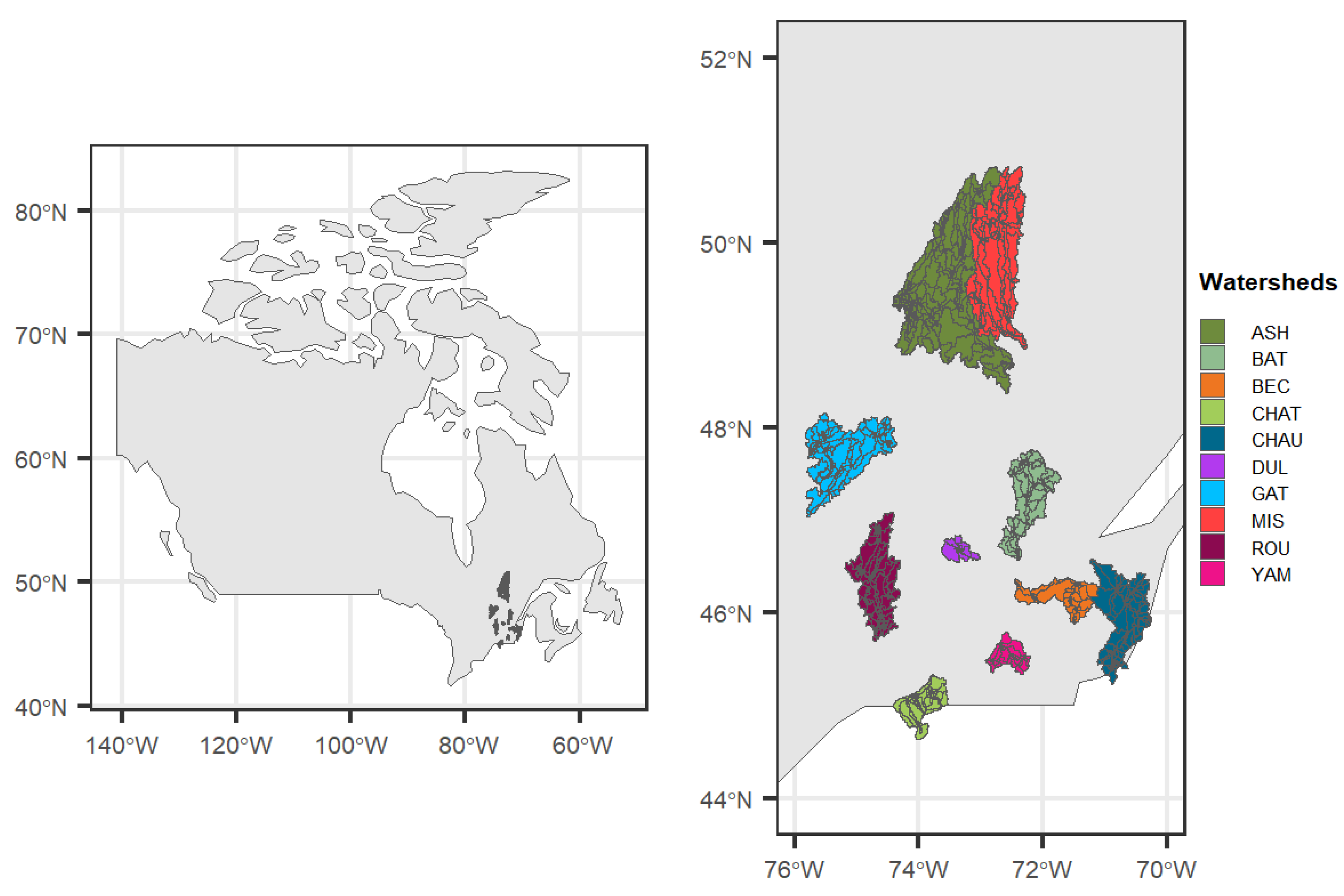
For this study, we considered several Canadian watersheds, namely Quebec’s Ashuapmushuan, Batiscan, Becancour, Chateauguay, Chaudière, Du Loup, Gatineau, Mistassini, Rouge, and Yamaska rivers (Figure 1). The data for the Quebec watersheds were provided by Foulon (2018) [29] as presented in Foulon and Rousseau (2018) [30]. They include two watersheds per hydrological region within the province of Québec. Based on their hydroclimatic regimes, these watersheds can be categorized into three distinct groups. Group (a) includes the Ashuapmushuan, Gatineau, and Mistassini watersheds, with the freshet peak and subsequent recession generally occurring during the first half of May. They are located north of the 47th parallel and encompasses boreal climates with warm or cold summers, based on the reanalyzed Köppen–Geiger classification [31]. Group (b) includes the Batiscan, Chaudière, and Du Loup watersheds, experiencing peak flows during the first half of April, which may persist until late April. They are characterized by boreal climates with warm summers, located on the south shore of the St. Lawrence River. Finally, Group (c) contains the Bécancour, Châteauguay, and Yamaska watersheds, with peak flows and recession phases that generally occur between late April and early May. They are characterized by boreal climates with warm summers, located on the north shore.

Most Quebec watersheds consist of deciduous and coniferous vegetations (i.e., forest) featuring large open spaces (i.e., mainly farmland and brushes) and vary greatly in vegetation types and surface areas.

Table 1. Land Use (% and km²) for the studied watersheds in Quebec.

Watershed/Land Use	Deciduous Vegetation (%)	Coniferous Vegetation (%)	Open Areas (%)	Total Area (km2)
Ashuapmushuan (ASH)	79.0	5.2	15.8	15,490
Batiscan (BAT)	34.1	27.4	38.5	4365
Becancour (BEC)	43.8	5.3	50.8	2723
Chateauguay (CHAT)	40.7	2.8	56.5	2477
Chaudière (CHAU)	42.0	12.2	45.7	5786
Du Loup (DUL)	39.0	18.1	42.9	855
Gatineau (GAT)	76.0	17.0	7.0	6830
Mistassini (MIS)	81.8	6.0	12.2	9603
Rouge (ROU)	69.2	25.4	5.4	5482
Yamaska (YAM)	41.5	0.9	57.6	1474

provides a summary of these characteristics for each basin. Land cover/land use data were obtained from the GlobCover project (2009).

2.4. Meteorological Data

Table 2. Averaged minimum (January) and maximum (July) temperatures and total annual precipitation for the period 1981/2010 for the various watersheds studied [32,33,34,35,36,37,38,39,40].

Watershed	Nearby Weather Station	Tmin (°C)	Tmax (°C)	Annual Precipitation (mm)
Ashuapmushuan	Hemon	−26.6	23.8	989
Batiscan	Lac aux Sables	−19.5	25.1	1133
Becancour	St Ferdinand	−17.5	24.0	1228
Chateauguay	Ormstown	−13.8	26.1	965
Chaudière	St Ludger	−16.7	23	1086
Du Loup	St Alexis des Monts	−19.7	25.6	1072
Gatineau	Ste Anne du Lac	−21.1	24.4	1040
Mistassini	Hemon	−26.6	23.8	989
Rouge	La Macaza	−19.5	25.1	1029
Yamaska	Granby	−14.2	25.2	1215

presents the average minimum and maximum monthly temperatures, as well as total annual precipitation, estimated over the 1981–2010 reference period for the selected watersheds [32,33,34,35,36,37,38,39,40]. While maximum monthly temperatures are relatively homogeneous across watersheds, with values close to 25 °C, minimum monthly temperatures exhibit substantial variability, ranging from −26.6 °C to −13.8 °C. Annual precipitation totals also vary markedly, from 965 mm to 1228 mm. These climatic conditions are typical of northern temperate and boreal environments [41].

2.5. Hydrometric Data

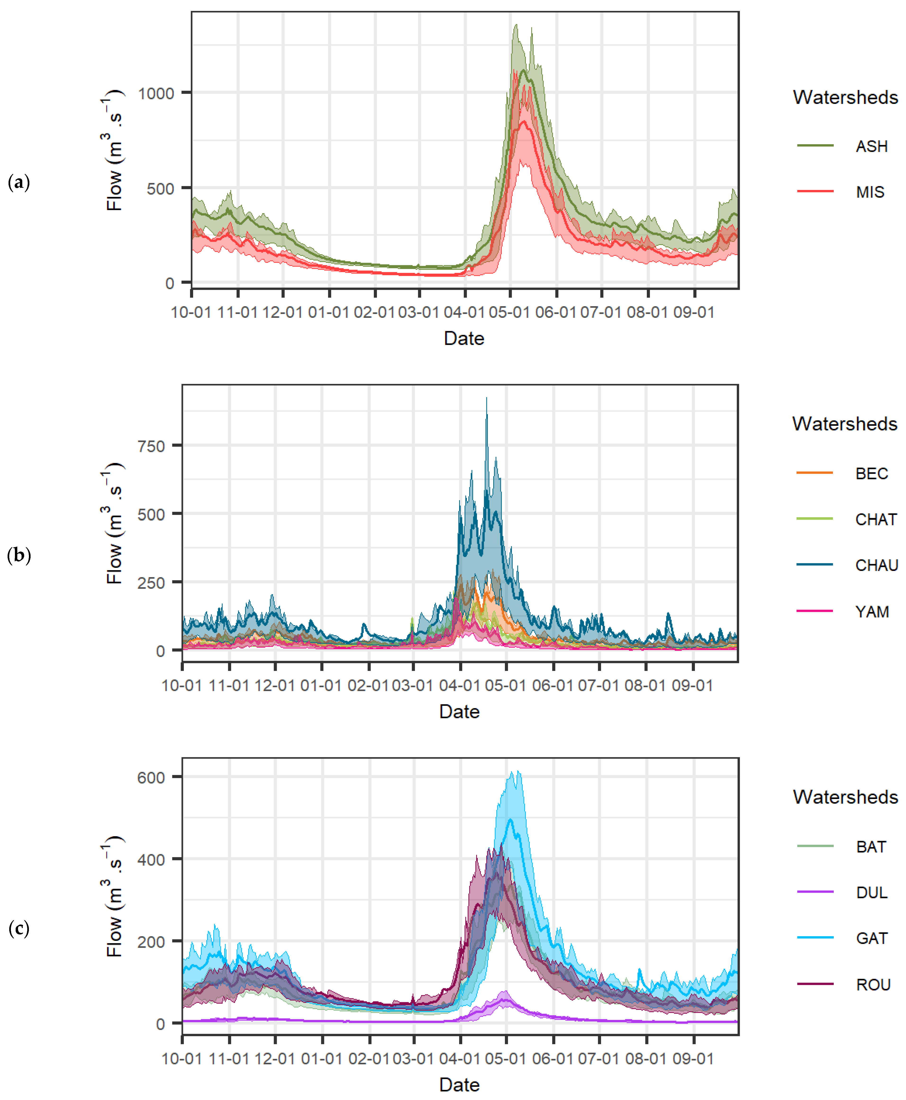
The study area encompasses ten watersheds in Québec, Canada. While these basins collectively share the climatic hallmarks of northern temperate and boreal environments, most notably long, snow-dominated winters, they also represent a significant spectrum of hydrological regimes. The ‘contrasts’ mentioned are the result of latitudinal and longitudinal gradients that dictate the frequency of rain-on-snow events and the duration of the spring freshet. By capturing this internal diversity within a broadly similar climatic envelope, we ensure a robust testbed for the two snow model configurations. Figure 2 illustrates the mean daily observed discharge, averaged over the available observation periods, for three groups of watersheds. Overall, freshets last approximately three months, including about one month of rising flows and roughly 75 days of falling limb.

To maximize data availability, hydrological years were defined from 1 October to 30 September.

Table 3. Q_7min and Q_7max for the various watersheds in m³·s⁻¹ and L·s⁻¹·km⁻² over their years of observed data. They refer, respectively, to the mean annual 7-day minimum and maximum flows calculated from raw daily observations, reflecting seasonal extremes rather than interannual means.

Watersheds	Q7min (m3·s−1/L·s−1·km−2)	Q7max (m3·s−1/L·s−1·km−2)
Ashuapmushuan	77/5	1274/82
Batiscan	22/5	480/110
Becancour	6/2	340/125
Chateauguay	4/2	284/115
Chaudière	10/2	875/151
Du Loup	2/2	78/91
Gatineau	27/4	629/92
Mistassini	39/4	1081/113
Rouge	24/4	511/93
Yamaska	1/0.7	189/128

reports the minimum and maximum 7-day average discharges (Q_7min and Q_7max) for each watershed over their respective observation periods. These values reflect the strong influence of watershed size on discharge magnitude, with Q_7min ranging from 1.4 to 76 m³ s⁻¹ and Q_7max from 78 to 1274 m³ s⁻¹.

2.6. Framework of the Study

The calibration period extended from 1 October 1981, to 30 September 1989, following a warm-up period beginning on 1 January 1981. The validation period covered 1 October 1990, to 30 September 2002, except for the Bécancour watershed, where data were available up to 30 September 2001. Due to gaps in observed discharge records, the validation period was interrupted on 30 September 1993, and resumed after a new warm-up period from 1 January 1997, to 30 September 1998. Freshet observations may be affected by river ice conditions. To minimize the influence of measurement uncertainty associated with ice cover, model evaluation was restricted to 15 March to 15 November of each year.

Table 4. Calibration parameters for the various modules of HYDROTEL and their ranges of variation.

Code (Unit)	Parameter	Module	Lower Limit of Calibration Range	Upper Limit of Calibration Range
PPN (°C)	Precipitation separation threshold temperature	Data interpolation	−5	5
GRADP (mm/100 m)	Vertical precipitation gradient	Data interpolation	0.1	3
GRADT (°C/100 m)	Vertical temperature gradient	Data interpolation	−1.2	−0.4
TFSN (mm/j)	Melting rate at ground/snow interface	Snow	0.1	2
DMAX (kg·m−3)	Maximum density of snow cover	Snow (« Mo »)	400	550
CTAS (-)	Settling coefficient	Snow	0.0001	0.1
TSFC (°C)	Temperature threshold for melting at the atmosphere/snow interface in coniferous environments	Snow	TSFF	TSFF + 5
TSFF (°C)	Melting temperature threshold at the atmosphere/snow interface in deciduous environments	Snow	−3	3
TSFO (°C)	Temperature threshold for melting at the atmosphere/snow interface in an open environment	Snow	TSFF—5	TSFF
TFANC (mm/j)	Melting rate at the atmosphere/snow interface in coniferous environments	Snow	0.5 × TFANF	TFANF
TFANF (mm/j)	Melting rate at the atmosphere/snow interface in deciduous environments	Snow	1	20
TFAN (mm/j)	Melting rate at the atmosphere/snow interface in open areas	Snow	TFANF	2 × TFANF
SCOUC (mm)	Threshold for creating snowpack layers in coniferous environments	Snow (« Multi »)	max(SCOUF,0)	100
SCOUF (mm)	Threshold for creating snowpack layers in deciduous environments	Snow (« Multi »)	max(SCOUD,0)	100
SCOUD (mm)	Threshold for creating snowpack layers in open areas	Snow (« Multi »)	0	100
FTEP (-)	Multiplier coefficient for PET optimization	Penman-Monteith	0.5	1.5
Z1 (m)	Ground 1st layer thickness	BV3C	0.025	0.6
Z2 (m)	Ground 2nd layer thickness	BV3C	max(Z1,0.05)	1.5
Z3 (m)	Ground 3rd layer thickness	BV3C	max(Z2,0.5)	3
CR (m/h)	Recession coefficient	BV3C	3.3 × 10−8	2 × 10−3

presents the calibrated parameters, their ranges of variation, the associated HYDROTEL modules, and their applicability to the different snow model configurations. While the Multi configuration uses 20 parameters compared to 18 for the Mo version, this two-parameter increase is more of a technical exchange than a simple addition. We kept the soil discretization parameters (Z1, Z2, Z3) consistent across both setups since they are core to the BV3C subsurface module. The real change lies in the snow physics: we added three land-cover-specific thresholds (SCOUD, SCOUF, SCOUC) to handle layering but were able to eliminate the DMAX parameter used in the Mo model.

Model calibration was performed using the OSTRICH optimization framework [42], which supports a variety of automated calibration algorithms. The Pareto Archived Dynamically Dimensioned Search (PADDS) algorithm [43] was selected due to its efficiency in multi-objective calibration problems. Two objective functions were used to assess model performance: the Kling–Gupta Efficiency (KGE, Equation (1)) [44], which emphasizes the reproduction of high flows, and the logarithmic Nash–Sutcliffe Efficiency (NSE_log, Equation (2)) [45], which is more sensitive to low-flow conditions.

$$KGE=1-{\left[{\left({\displaystyle \frac{{\mu }_s}{{\mu }_o}}-1\right)}^2+{\left({\displaystyle \frac{{\sigma }_s}{{\sigma }_o}}-1\right)}^2{+\left(r-1\right)}^2\right]}^{{\displaystyle \frac{1}{2}}}$$

(1)

where ${\mu }_s$ and ${\mu }_o$ are the means of the simulated (s) and observed (o) series,

${\sigma }_s$ and ${\sigma }_o$ are the standard deviations of the simulated and observed series,

r is the Pearson correlation coefficient.

$${NSE}_{log}=1-{\displaystyle \frac{{\sum }_{i=1}^n{\left(log\left(Q_{s,i}\right)-log\left(Q_{o,i}\right)\right)}^2}{{\sum }_{i=1}^n{\left(log\left(Q_{o,i}\right)-log\left(\overline{Q_o}\right)\right)}^2}}$$

(2)

where $Q_{s,i}$ and $Q_{o,i}$ are the simulated flow (s) and observed flow (o) at time step i,

$\overline{Q_o}$ is the average of observed flows.

Following the recommendations of Tolson and Shoemaker (2007) [46], ten independent calibration trials of 200 iterations were performed for each model configuration, yielding ten Pareto fronts. The dominant solutions from these fronts were combined into a single Pareto front using a non-dominated sorting approach. Optimal parameter sets were selected based on their ability to balance KGE and NSE_log performance during both calibration and validation periods. Model performance was statistically compared using the Wilcoxon rank-sum test, applied to the medians of performance metrics obtained for each model configuration. This non-parametric test was used to determine whether differences in performance between the Mo and Multi models were statistically significant across watersheds and evaluation periods. In addition to overall performance, KGE and NSE_log were evaluated separately for the rising and the falling limbs of the freshet hydrograph. The rising limb covers the period from the onset of the freshet to the peak flow, while the falling limb spans the period from the peak flow to the end of the event. To evaluate freshet dynamics, we used the non-parametric Pettitt change-point test [47] to split the hydrograph into its rising and falling limbs. This gave us a much more targeted look at how the model performs during specific stages of the melt season. Once the date of the annual snowmelt-driven maximum discharge was identified, the test was applied between March 15 and the peak date to detect the onset of the rising limb, and between the peak date and August 1 to identify the end of the freshet. Finally, several hydrological indicators were assessed at the watershed scale, including annual cumulative freshet volume, annual maximum discharge and timing, and freshet starting and ending dates. Linear regressions between observed and simulated values were computed over the entire observation period for each indicator. Regression slopes, coefficients of determination, and relative biases were compared between model configurations, and differences in regression slopes were assessed using the Welch t-test [48].

3. Results

3.1. Overall Performances

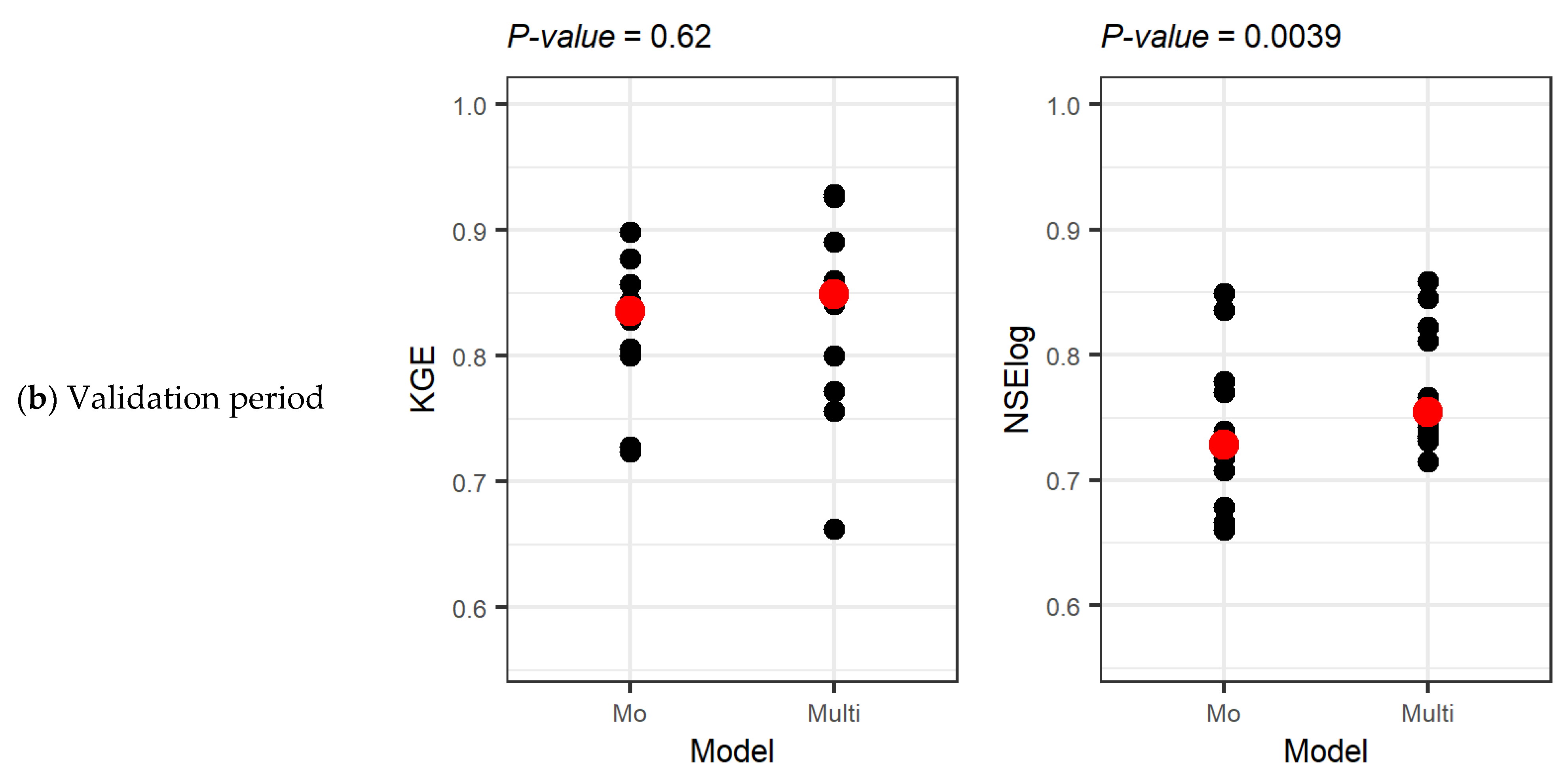
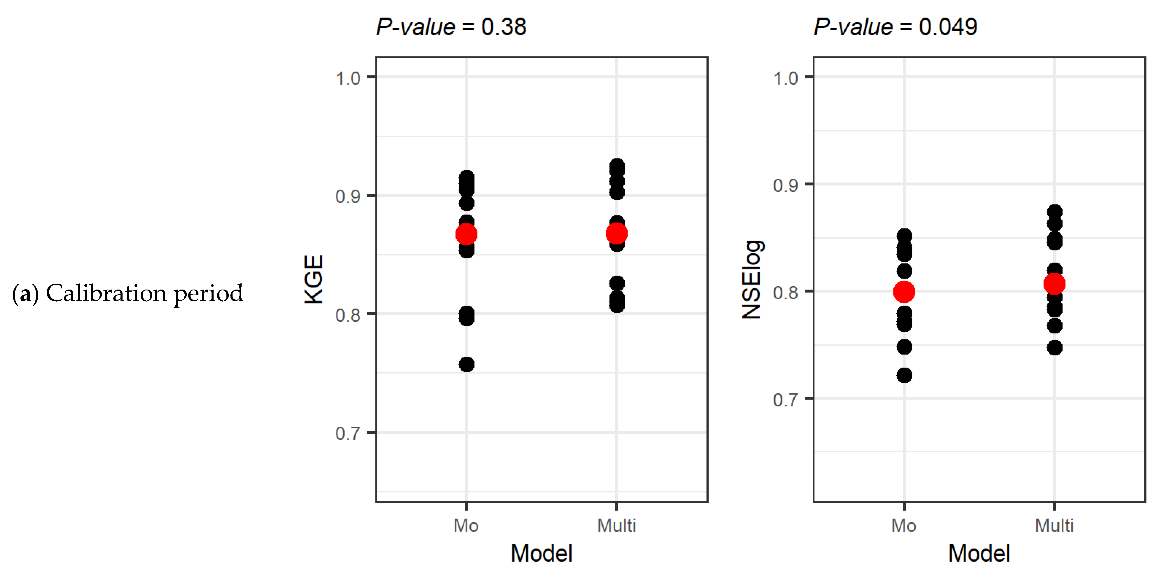
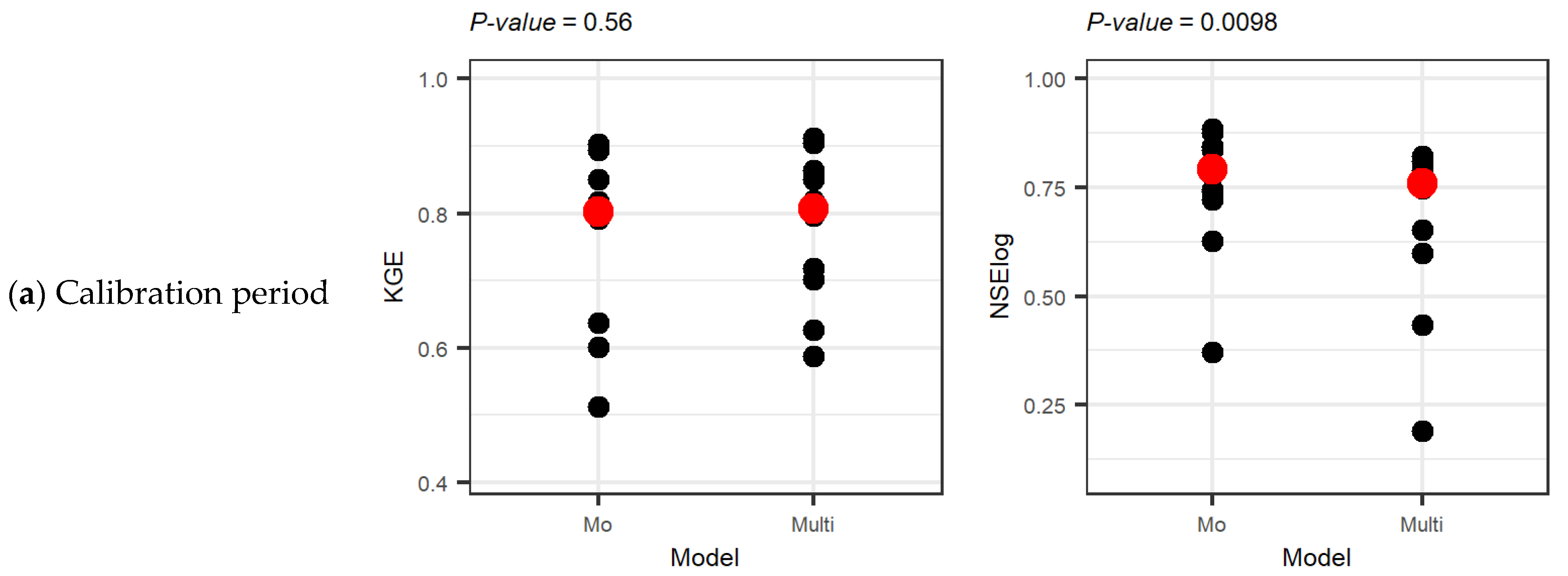
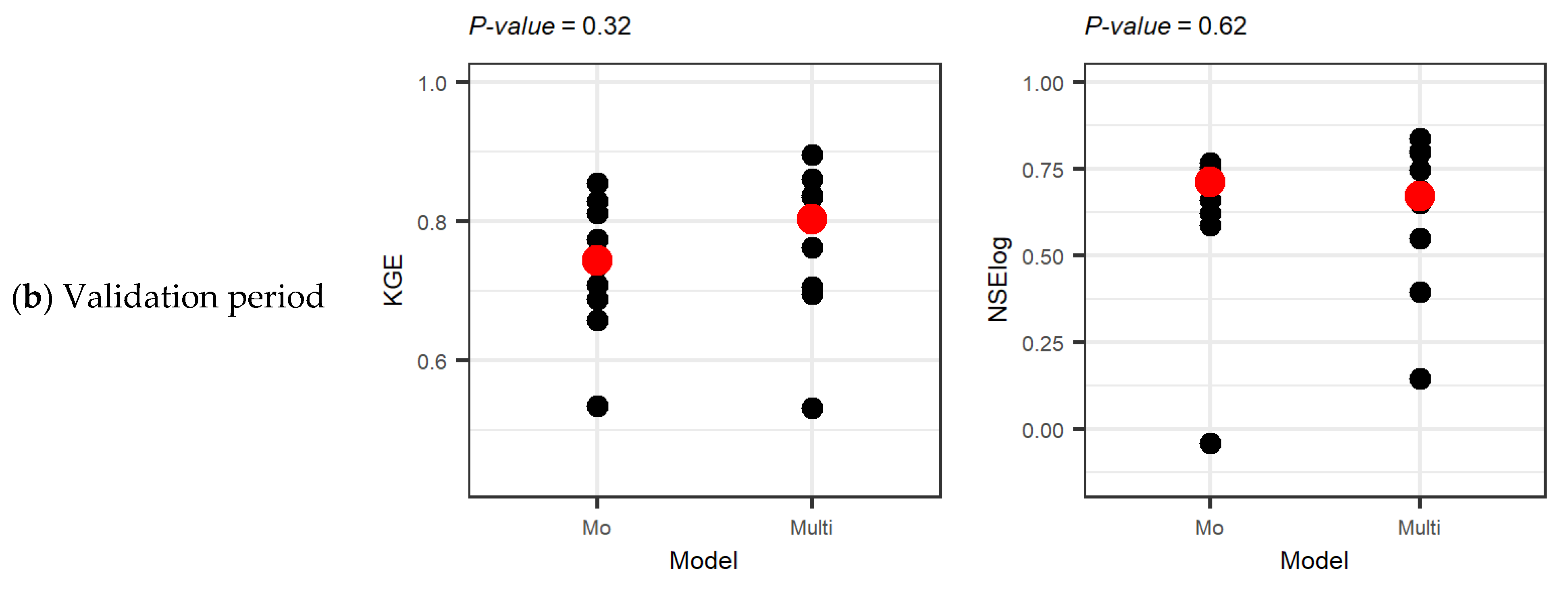
As a first step, overall model performance was assessed across the full range of flow conditions. Streamflow simulations obtained with both snow model configurations are presented in Supplementary Information Part S1.1. Figure 3 illustrates the distribution of Kling–Gupta Efficiency (KGE) and the logarithmic Nash–Sutcliffe Efficiency (NSE_log) values obtained for the Mo and Multi models across the ten watersheds for the calibration and validation periods.

The Wilcoxon signed-rank test applied to the calibration period yielded a p-value of 0.38 for the KGE and 0.049 for the NSE_log (median NSE_log for Mo:0.80; for Multi:0.81). For the validation period, p-values were 0.63 for the KGE and 3.9 × 10⁻³ for the NSE_log (median NSE_log for Mo:0.73; for Multi:0.75). These results indicate that, at the 5% significance level, there is not any statistically significant difference between the two models for the KGE values, whereas a significant difference is observed for the NSE_log.

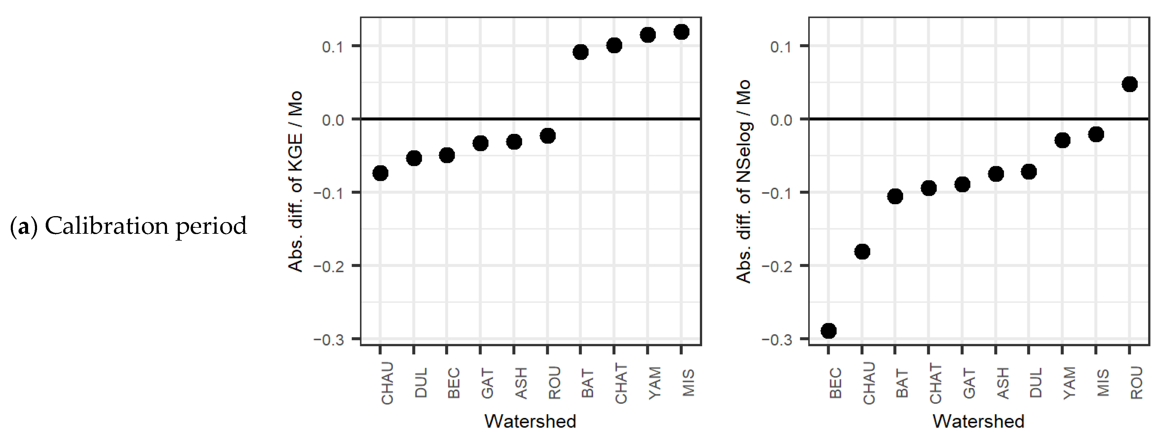
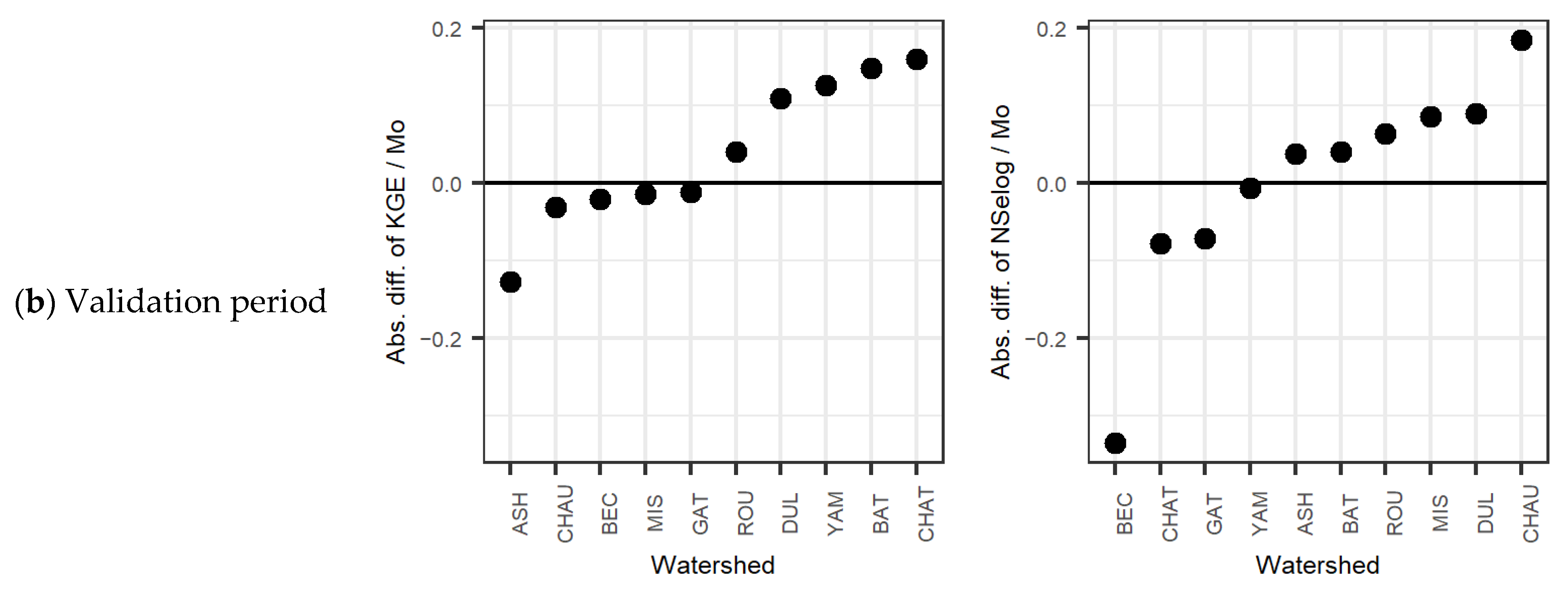
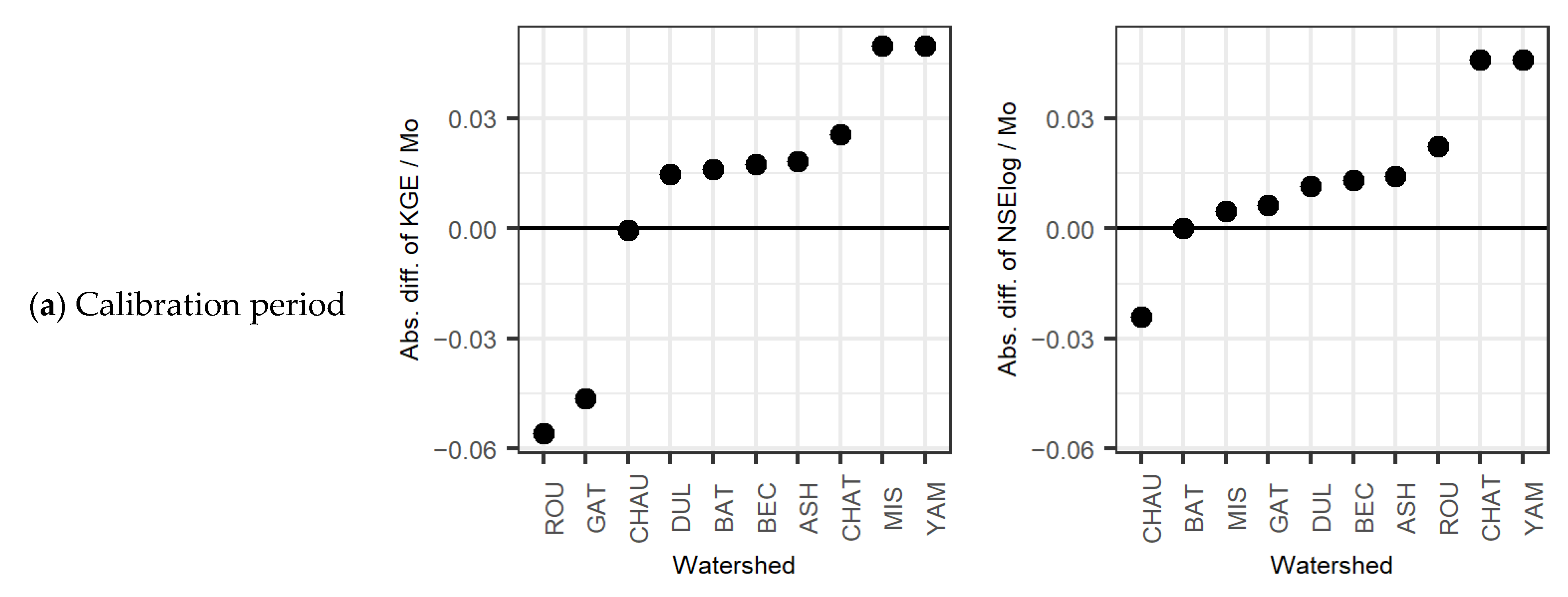
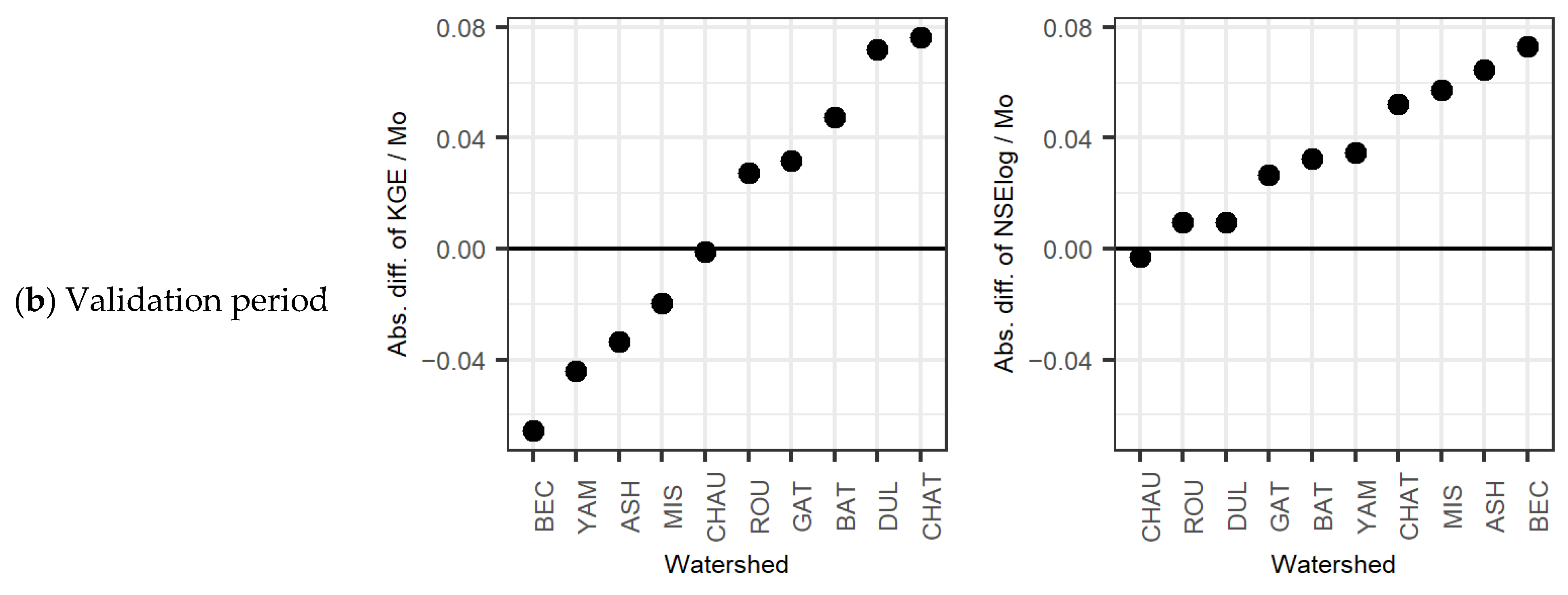
These results suggest that, while overall streamflow performance remains comparable between the two model configurations, the multilayer snow model exhibits a slight but consistent improvement in low-flow simulation. To further investigate whether this improvement is uniformly distributed across watersheds, differences in performance metrics were examined individually for each basin. Figure 4 presents the absolute differences in KGE and NSE_log between the Mo and Multi models across all watersheds for both (a) calibration and (b) validation periods. Watersheds are sorted in ascending order to emphasize relative improvements in model performance.

Figure 4 shows that no systematic superiority of one model over the other is evident based on the KGE. On the other end, most watersheds exhibit higher NSE_log values for the multilayer model for both calibration and validation periods, with maximum improvements reaching 0.07. This pattern supports the hypothesis that the multilayer snow model primarily enhances low-flow simulations rather than high-flow performances. The transition to the multilayer scheme allowed for a dynamic discretization of the snowpack’s internal structure. Throughout the peak accumulation period, the calibration process consistently produced between 1 and 8 snow layers across the study watersheds.

3.2. Rising and Falling Limbs of the Freshet Hydrograph

Differences between the snow model configurations may be more apparent when focusing specifically on the dynamics of the freshet. Figure 5 presents the KGE and NSE_log values obtained for the Mo and Multi models during the rising limb period for both the calibration and validation phases.

During the rising limb of the freshet period, median values indicate that the multilayer model yields slightly higher KGE values but lower NSE_log values than the monolayer model. Among the four Wilcoxon signed-rank tests conducted, only one test was statistically significant: the NSE_log for the calibration period (median NSE_log for Mo:0.79; for Multi:0.76).

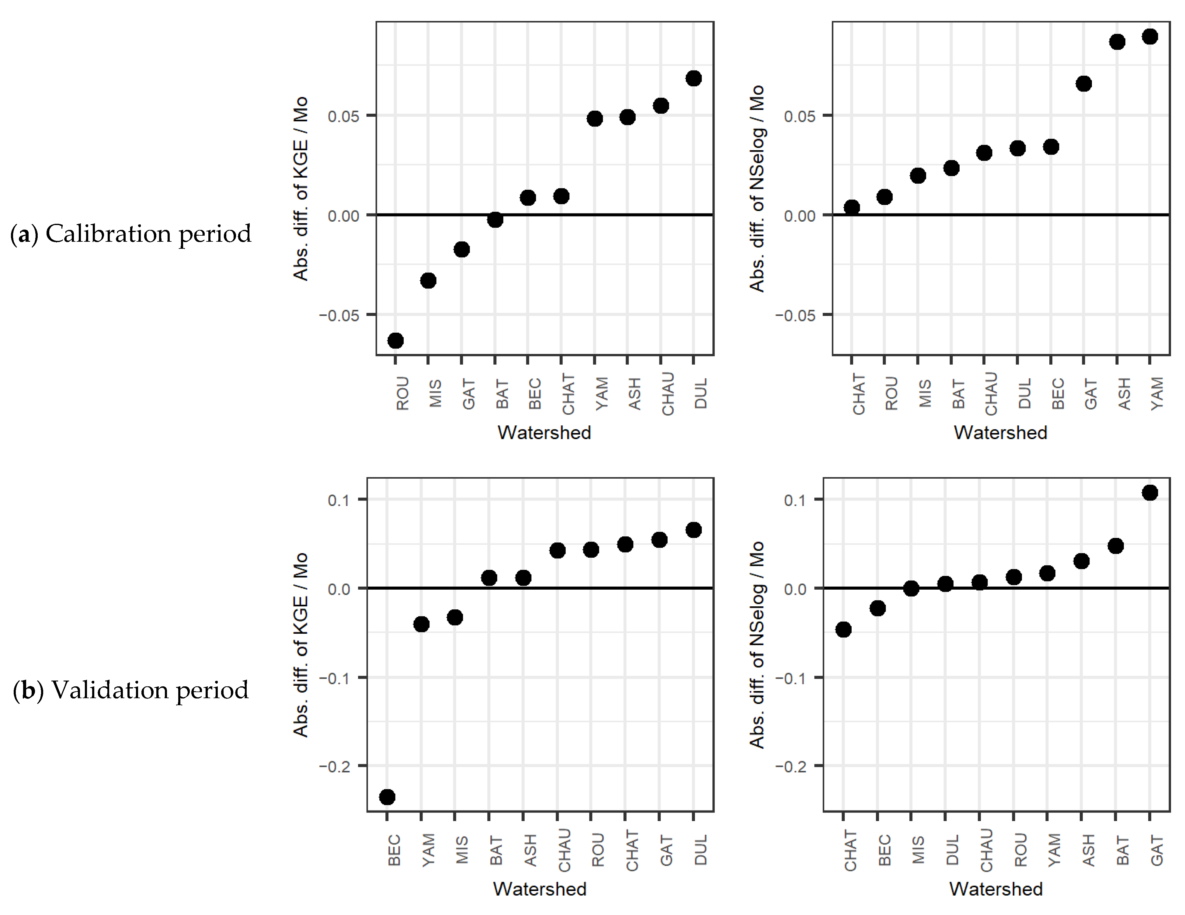
These results indicate that the monolayer model slightly outperforms the multilayer model during low-flow conditions prior to peak of the freshet for the calibration period, with a median difference of approximately 0.03. To further explore watershed-specific behavior, Figure 6 illustrates the relative and absolute differences in performance between the Multi and Mo models for: (a) the calibration and (b) the validation periods. Watersheds are sorted in ascending order to highlight gains in performance.

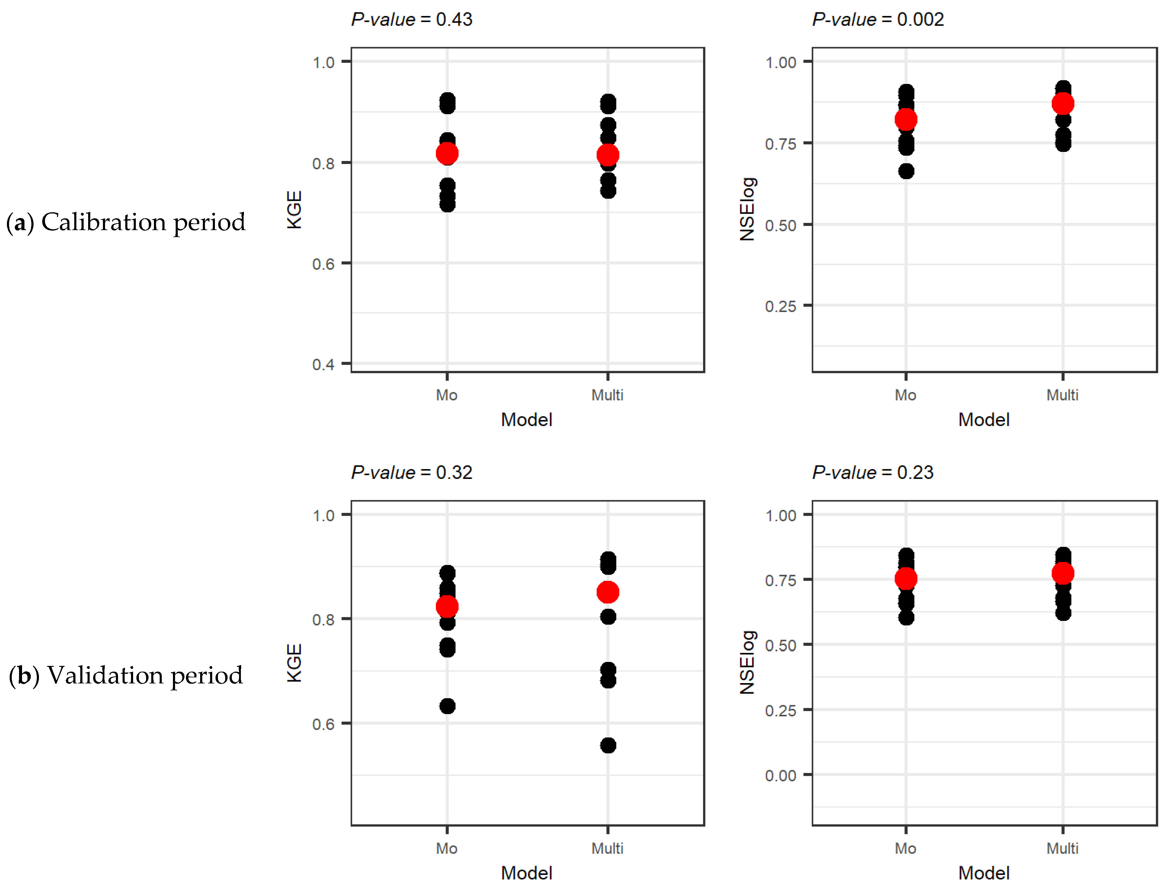
Figure 6 shows that improvement in KGE values vary across watersheds, with neither model consistently outperforming the other. A similar pattern is observed for the NSE_log for the validation period. However, during the calibration period, the monolayer model exhibits a more pronounced advantage in NSE_log across most watersheds, which explains the statistically significant result observed in Figure 5. Figure 7 presents the KGE and NSE_log results for the falling limb period for both snow model configurations for the calibration and validation phases.

For the falling limb period, the Wilcoxon signed-rank test yields p-values of 0.43 for the KGE and 2.0 × 10⁻³ for the NSE_log (median NSE_log for Mo:0.82; for Multi:0.87) during the calibration period, and 0.32 for the KGE and 0.23 for the NSE_log during the validation period. These results indicate a statistically significant improvement in NSE_log values for the calibration period when using the multilayer snow model.

The multilayer model exhibits a median NSE_log increase of approximately 0.05 for the calibration period, which is statistically significant, whereas the increase observed for the validation period (0.02) is not statistically significant. Figure 8 presents the relative and absolute differences in KGE and NSE_log between the two model configurations for each watershed for: (a) the calibration and (b) the validation periods. Watersheds are sorted to emphasize performance improvements.

Figure 8 shows that neither model consistently outperforms the other in terms of KGE for the calibration period or NSE_log for the validation period. However, for the NSE_log for the calibration period, the multilayer model outperforms the monolayer model across all watersheds, explaining the statistically significant improvement observed in Figure 7. Overall, statistically significant differences between the two snow model configurations are primarily associated with NSE_log for the calibration period, both for the rising and falling limbs periods. Because this metric is particularly sensitive to low-flow conditions, these results motivate a more detailed examination of flood-related hydrological indicators, and this is addressed in the following section that focusses on how the multilayer snow model influences the dynamics of the freshet.

3.3. Analysis of Annual Runoff Volume and Maximum Discharges of the Freshet

Linear regressions were computed between modeled and observed values for each characteristic at the watershed scale. Figures and tables summarizing these regressions are provided in Supplementary Information Parts S1.2 to S1.6 for continuity. The regression analyses indicate that none of the regression slopes differ significantly between the two model configurations for any of the evaluated characteristics.

Despite the absence of statistically significant differences, several indicators suggest a slight advantage of the multilayer snow model for specific flood-related characteristics. These tendencies are summarized in

Table 5. Average absolute differences between modeled and observed flood-related characteristics, expressed in terms of regression slope error and relative bias.

	Slope		Bias
Characteristics	Mo	Multi	Mo	Multi
Annual cumulative freshet volume	0.157	0.121	13.5	8.83
Freshet starting date	0.0123	0.0178	1.23	1.77
Freshet ending date	0.0199	0.0197	1.76	1.67
Dates of annual maximum discharge	0.0207	0.0249	2.24	2.74
Annual maximum discharge	0.104	0.0754	8.99	7.06

, which presents the average absolute differences between the modeled regression slope (or relative bias) and the theoretical optimal value corresponding to a perfect model.

Looking at the annual flood characteristics in Table 5, it becomes clear that both configurations similarly handle the freshet timing. However, the multilayer model distinctly improved the volumetric accuracy. Even though the regression slopes did not quite meet the p < 0.05 significance level, we consistently achieved lower relative biases with the multilayer approach for both peak discharges and cumulative volumes.

4. Discussion

Moving from a monolayer to a multilayer snow module does add three calibration parameters (SCOUC, SCOUF, and SCOUD), but they are not arbitrary values. They act as constrained physical thresholds for snowpack discretization based on land use. For models like HYDROTEL, the traditional concern about over-parameterization is offset by a drop in structural error. By explicitly modeling internal layers, the “Multi” setup offers a much more realistic approach to energy transfer and meltwater. This physical grounding circumvents up to a point the “equifinality” trap where simpler models fall into (p < 0.004). Thus, for the “Multi” setup, it is a sign of robustness since the model captured a real hydrological signal rather than just overfitting.

The objective of this article was to assess the potential of adaptations recently proposed for the HYDROTEL snow module to improve streamflow modeling during freshet. The implementation of these adaptations showed an improvement in snowmelt modeling and, consequently, in streamflow modeling. Taken together, these results suggest that the main benefit of the multilayer snow model lies in a more coherent temporal distribution of snowmelt contributions to streamflow, rather than in a systematic improvement of peak discharge magnitude. This distinction is essential for interpreting the added value of increased snow model complexity.

Existing literature indicates that a multilayer snow model generally improves snowpack simulation, but that this improvement is not always discernible at the annual scale when evaluating streamflow modeling performance. These results are consistent with previous studies showing that improvements in snow physics do not necessarily translate into significant gains in annual discharge metrics. Indeed, Avanzi et al. (2016) [49] demonstrated that the multilayer snow model CROCUS outperforms the monolayer HyS snow model, despite comparable cumulative runoff. Carletti et al. (2022) [50] observed that the monolayer snow model of the Poli-Hydro framework shows comparable seasonal flow performance to that of the Alpine3D framework, which applies the multilayer snow model SNOWPACK to each catchment cell. Zsoter et al. (2022) [51] presents a slight improvement of the ECLand model, thanks to a multilayer snow scheme, where the KGE improved by 0.03 on average for 453 catchments. The results of our study align with this existing literature.

The ‘slight’ improvements in KGE values observed in this study should not be viewed as a lack of model efficacy, but rather as a reflection of the inherent limits of peak-flow sensitivity to vertical snow layering. Our findings reproduce the ‘complexity-performance plateau’ identified by Avanzi et al. (2016) [49]. While a monolayer model can often be calibrated to match a hydrograph peak through parameter compensation, the multilayer approach achieves comparable (and often superior) results by reducing structural uncertainty. Specifically, the reduction in volume bias (Table 5) and the jump in NSE_log during the falling limb suggest that the multilayer framework better simulates the physical ‘ripening’ and depletion of the snowpack, providing a more reliable foundation for water management than simple conceptual models.

By focusing on the freshet rising and falling limbs period, differences between the two snow model configurations become more apparent. For the rising limb period, the original monolayer snow model slightly outperforms the multilayer configuration, whereas over the falling limb period, the multilayer snow model yields better results. We should contextualize the Mo model’s rising-limb performance within the structural logic of HYDROTEL, where infiltration only begins after total snow depletion. The monolayer configuration often melts out rapidly and uniformly, triggering soil recharge sooner than its multilayer counterpart. However, the Multi model’s ability to simulate internal refreezing and water retention naturally extends the life of the snowpack. Although this might appear as a delay in infiltration, the payoff is a 35% improvement in cumulative volume accuracy (Table 5). This is because the multilayer approach captures the internal ripening of the snowpack as it accounts for the energy required to warm the lower layers to 0 °C before the final melt occurs. By providing a more precise mass balance, the Multi model creates a more robust soil moisture state for the falling limb. This directly accounts for the statistically significant improvements in NSE_log observed during the later stages of the freshet.

In addition, several flood-related characteristics were evaluated to assess the ability of both snow model configurations to reproduce key hydrological indicators. The results show that the multilayer snow model slightly improves streamflow modeling during the freshet, particularly for cumulative freshet volumes. The apparent improvement in maximum discharge does not correspond to a systematic improvement in flood peak simulation but rather reflects a better representation of meltwater contribution over the freshet period. These results highlight the importance of accurately representing snowpack processes to improve freshet volume estimation.

The 35% reduction in the bias of the cumulative freshet volume is a perfect example of practical utility outweighing strict statistical significance. For real-world water management, a 4.7% absolute bias reduction (Table 5) represents a significant step forward for “internal mass balance”. This gain shows that the multilayer setup handles snow-melt-to-streamflow partitioning more effectively, a vital factor for water resources planning and flood risks, where total volume errors can be just as damaging as missing peak timing.

Finally, the multilayer snow model also improves the simulation of the end of the freshet period, contributing to a more likely representation of snowmelt depletion. This improvement is particularly relevant for applications requiring an accurate description of seasonal flow transitions. Despite the study’s limited number of watersheds, the findings are consistent with existing literature. Expanding the study to include a larger number of watersheds, with diverse drainage areas and climatic conditions, would contribute to a more robust statistical results and enhance the generalizability of the findings.

5. Conclusions

The snow model of the hydrological model HYDROTEL is structured to simulate snow accumulation and melt processes using a monolayer approach. Recent developments have proposed several adaptations focusing on an improved physical representation of the snowpack, including the implementation of a multilayer structure. This study assessed the added-value of these adaptations with respect to streamflow modeling across ten (10) snow-dominated watersheds in Quebec, Canada. Two snow model configurations were compared: the original monolayer model and a multilayer model incorporating recent developments. Results indicate that overall streamflow performance remains similar for both configurations at the annual scale. However, when focusing on freshet dynamics, differences between them become more evident. For the freshet rising limb, the monolayer snow model slightly outperforms the multilayer configuration, whereas for the falling limb period, the multilayer snow model provides improved performances, particularly for low-flow conditions. Although the annual statistical improvements are subtle, correcting the systematic volumetric bias represents a significant step forward. It highlights the added value of multilayer physics for any real-world application where cumulative water volumes are a priority. For operational forecasting, this reduction in bias is arguably more important than the broader statistical metrics. These results suggest that the multilayer snow model improves the temporal distribution of snowmelt contributions. The analysis of flood-related characteristics further shows that the multilayer snow model slightly improves the simulation of cumulative freshet volumes and maximum discharge. These improvements are achieved without degrading overall streamflow performance. In the end, the results indicate that increasing the physical realism of the snow model improves the representation of snowmelt-driven runoff processes, particularly during the falling limb period. Importantly, the proposed multilayer snow model does not aim to systematically improve flood peak simulation, but rather to enhance the internal consistency of snowmelt-driven runoff processes. While the gains in timing (KGE) are currently limited by how HYDROTEL handles the snow-soil interface, the multilayer module still manages to reduce structural uncertainty. It simply provides a more mass-consistent look at the snowpack. This confirms that the multilayer physics are already capturing the primary dynamics; if we were to refine the infiltration logic in the future, perhaps by allowing infiltration at the soil-snowpack interface before the snowpack fully melts, the benefits of this new physics would be even more pronounced. As such, the added value is most relevant for applications sensitive to seasonal transitions, cumulative volumes, and low-flow conditions. Future work could further investigate the sensitivity of these results to climate variability and explore the potential benefits of multilayer snow models under changing winter conditions, such as increased rain-on-snow events or altered heat balance within the snowpack.

References

1. Li, D.; Wrzesien, M.L.; Durand, M.; Adam, J.; Lettenmaier, D.P. How much runoff originates as snow in the western United States, and how will that change in the future? Geophys. Res. Lett. 2017, 44, 6163–6172. [Google Scholar] [CrossRef]
2. Jasechko, S.; Wassenaar, L.I.; Mayer, B. Isotopic evidence for widespread cold-season-biased groundwater recharge and young streamflow across central Canada. Hydrol. Process. 2017, 31, 2196–2209. [Google Scholar] [CrossRef]
3. Liang, X.; Lettenmaier, D.P.; Wood, E.F.; Burges, S.J. A simple hydrologically based model of land surface water and energy fluxes for general circulation models. J. Geophys. Res. 1994, 99, 14415–14428. [Google Scholar] [CrossRef]
4. Andreadis, K.M.; Storck, P.; Lettenmaier, D.P. Modeling snow accumulation and ablation processes in forested environments: VIC SNOW MODEL. Water Resour. Res. 2009, 45, 1–13. [Google Scholar] [CrossRef]
5. Arnold, J.G.; Srinivasan, R.; Muttiah, R.S.; Williams, J.R. Large Area Hydrologic Modeling And Assessment Part I: Model Development. J. Am. Water Resour. Assoc. 1998, 34, 73–89. [Google Scholar] [CrossRef]
6. Marsh, C.B.; Pomeroy, J.W.; Wheater, H.S. The Canadian Hydrological Model (CHM) v1.0: A multi-scale, multi-extent, variable-complexity hydrological model—design and overview. Geosci. Model Dev. 2020, 13, 225–247. [Google Scholar] [CrossRef]
7. Poissant, D.; Arsenault, R.; Brissette, F. Impact of parameter set dimensionality and calibration procedures on streamflow prediction at ungauged catchments. J. Hydrol. Reg. Stud. 2017, 12, 220–237. [Google Scholar] [CrossRef]
8. Krinner, G.; Derksen, C.; Essery, R.; Flanner, M.; Hagemann, S.; Clark, M.; Hall, A.; Rott, H.; Brutel-Vuilmet, C.; Kim, H.; et al. ESM-SnowMIP: Assessing snow models and quantifying snow-related climate feedbacks. Geosci. Model Dev. 2018, 11, 5027–5049. [Google Scholar] [CrossRef]
9. Turcotte, R.; Lacombe, P.; Dimnik, C.; Villeneuve, J.-P. Prévision hydrologique distribuée pour la gestion des barrages publics du Québec. Can. J. Civ. Eng. 2004, 31, 308–320. [Google Scholar] [CrossRef]
10. Turcotte, R. Elements du Calage et de L’implantation D’un Modele Hydrologique Dans Une Perspective D’utilisation Operationnelle en Prevision Hydrologique. Ph.D. Thesis, Université du Québec, Québec, QC, Canada, 2010. [Google Scholar]
11. Samuel, J.; Rousseau, A.N.; Abbasnezhadi, K.; Savary, S. Development and evaluation of a hydrologic data-assimilation scheme for short-range flow and inflow forecasts in a data-sparse high-latitude region using a distributed model and ensemble Kalman filtering. Adv. Water Resour. 2019, 130, 198–220. [Google Scholar] [CrossRef]
12. Rousseau, A.N.; Savary, S.; Tremblay, S.; Caillouet, L.; Doumbia, C.; Augas, J.; Foulon, É.; Abbasnezhadi, K. A Distributed Hydrological Modelling System to Support Hydroelectric Production in Northern Environment Under Current and Changing Climate Conditions; INRS-ETE: Québec, QC, Canada, 2020. [Google Scholar]
13. Abbasnezhadi, K.; Rousseau, A.N.; Foulon, É.; Savary, S. Verification of Regional Deterministic Precipitation Analysis Products Using Snow Data Assimilation for Application in Meteorological Network Assessment in Sparsely Gauged Nordic Basins. J. Hydrometeorol. 2021, 22, 859–876. [Google Scholar] [CrossRef]
14. Centre d’expertise hydrique du Québec (CEHQ). Atlas Hydroclimatique du Québec Méridional: Impact Des Changements Climatiques Sur Les Régimes de Crue, D’étiage et D’hydraulicité à L’horizon 2050; Gouvernement du Québec: Québec, QC, Canada, 2013.
15. Centre d’expertise hydrique du Québec (CEHQ). Atlas Hydroclimatique du Québec Méridional: Impact Des Changements Climatiques Sur Les Régimes de Crue, D’étiage et D’hydraulicité à L’horizon 2050; Centre D’expertise Hydrique du Québec, Ministère du Développement Durable, de L’environnement et de la lutte contre Les Changements Climatiques: Québec, QC, Canada, 2015. [Google Scholar]
16. Direction de l’expertise hydrique (DEH). Document D’accompagnement de L’atlas Hydroclimatique; Ministère du Développement Durable, de L’environnement et de la Lutte Contre Les Changements Climatiques: Québec, QC, Canada, 2018. [Google Scholar]
17. Direction de l’hydrologie et de l’hydraulique (DHH). Rapport Technique de l’Atlas Hydroclimatique du Québec Méridional; Ministère de l’Environnement, de la Lutte Contre Les Changements Climatiques, de la Faune et Des Parcs: Québec, QC, Canada, 2024. [Google Scholar]
18. Blanchette, M.; Rousseau, A.N.; Foulon, É.; Savary, S.; Poulin, M. What would have been the impacts of wetlands on low flow support and high flow attenuation under steady state land cover conditions? J. Environ. Manag. 2019, 234, 448–457. [Google Scholar] [CrossRef]
19. Wu, Y.; Zhang, G.; Rousseau, A.N.; Xu, Y.J. Quantifying streamflow regulation services of wetlands with an emphasis on quickflow and baseflow responses in the Upper Nenjiang River Basin, Northeast China. J. Hydrol. 2020, 583, 124565. [Google Scholar] [CrossRef]
20. Rousseau, A.N.; Savary, S.; Bazinet, M.-L. Flood water storage using active and passive approaches—Assessing flood control attributes of wetlands and riparian agricultural land in the Lake Champlain-Richelieu River watershed. In A Report to the International Lake Champlain-Richelieu River Study Board; INRS-Centre Eau Terre Environnement: Québec, QC, Canada, 2022. [Google Scholar]
21. Morin, G. Conception de Bandes Riveraines et de Retenues Collinaires à L’aide de la Modélisation Hydrologique Distribuée et Évaluation de L’impact de Ces Aménagements Sur la Charge en Sédiments. Master’s Thesis, Université du Québec, Institut national de la Recherche Scientifique, Québec, QC, Canada, 2023. [Google Scholar]
22. Fortin, J.-P.; Turcotte, R.; Massicotte, S.; Moussa, R.; Fitzback, J.; Villeneuve, J.-P. Distributed Watershed Model Compatible with Remote Sensing and GIS Data. I: Description of Model. J. Hydrol. Eng. 2001, 6, 91–99. [Google Scholar] [CrossRef]
23. Turcotte, R.; Rousseau, A.N.; Fortin, J.-P.; Villeneuve, J.-P. A process-oriented, multiple-objective calibration strategy accounting for model structure. In Water Science and Application; Duan, Q., Gupta, H.V., Sorooshian, S., Rousseau, A.N., Turcotte, R., Eds.; American Geophysical Union: Washington, DC, USA, 2003; Volume 6, pp. 153–163. [Google Scholar]
24. Turcotte, R.; Fortin, L.G.; Fortin, V.; Fortin, J.P.; Villeneuve, J.-P. Operational analysis of the spatial distribution and the temporal evolution of the snowpack water equivalent in southern Québec, Canada. Hydrol. Res. 2007, 38, 211–234. [Google Scholar] [CrossRef]
25. Augas, J.; Foulon, E.; Rousseau, A.N.; Baraër, M. Extension of a Monolayer Energy-Budget Degree-Day Model to a Multilayer One. Water 2024, 16, 1089. [Google Scholar] [CrossRef]
26. Rousseau, A.N.; Savary, S.; Tremblay, S. Développement de PHYSITEL 64 Bits Avec Interface Graphique Pour Supporter Les Applications d’HYDROTEL Sur Des Bassins Versants de Grande Envergure: (Incluant Des Compléments D’aide et Des Développements Pour HYDROTEL): Travaux 2016. Rapport Final; Institut National de la Recherche Scientifique-Centre Eau Terre Environnement: Québec, QC, Canada, 2017. [Google Scholar]
27. Barszcz, A.; Milbrandt, J.A.; Thériault, J.M. Improving the Explicit Prediction of Freezing Rain in a Kilometer-Scale Numerical Weather Prediction Model. Weather Forecast 2018, 33, 767–782. [Google Scholar] [CrossRef]
28. Myers, D.T.; Ficklin, D.L.; Robeson, S.M. Incorporating rain-on-snow into the SWAT model results in more accurate simulations of hydrologic extremes. J. Hydrol. 2021, 603, 126972. [Google Scholar] [CrossRef]
29. Foulon, E. Prédiction de L’état Futur de L’approvisionnement en Eau Potable de Surface: Mise au Point D’une Méthode D’évaluation Des Débits D’étiage à Partir de Données Climatiques. Ph.D. Thesis, Université du Québec, Institut National de la Recherche Scientifique, Québec, QC, Canada, 2018. [Google Scholar]
30. Foulon, É.; Rousseau, A.N. Equifinality and automatic calibration: What is the impact of hypothesizing an optimal parameter set on modelled hydrological processes? Can. Water Resour. J. Rev. Can. Des Ressour. Hydr. 2018, 43, 47–67. [Google Scholar] [CrossRef]
31. Rubel, F.; Brugger, K.; Haslinger, K.; Auer, I. The climate of the European Alps: Shift of very high resolution Köppen-Geiger climate zones 1800–2100. Meteorol. Z. 2017, 26, 115–125. [Google Scholar] [CrossRef]
32. Government of Canada. Environment and Climate Change Canada. Meteorological Station: Hemon, Québec. 2021. Available online: https://climat.meteo.gc.ca/climate_normals/results_1981_2010_f.html?stnID=5909&autofwd=1 (accessed on 24 March 2021).
33. Government of Canada. Environment and Climate Change Canada. Meteorological Station: Lac Aux Sables, Québec. 2021. Available online: https://climat.meteo.gc.ca/climate_normals/results_1981_2010_f.html?stnID=5203&autofwd=1 (accessed on 24 March 2021).
34. Government of Canada. Environment and Climate Change Canada. Meteorological Station: St Ferdinand, Québec. 2021. Available online: https://climat.meteo.gc.ca/climate_normals/results_1981_2010_f.html?stnID=5463&autofwd=1 (accessed on 24 March 2021).
35. Government of Canada. Environment and Climate Change Canada. Meteorological Station: Ormstown, Québec. 2021. Available online: https://climat.meteo.gc.ca/climate_normals/results_1981_2010_f.html?stnID=5429&autofwd=1 (accessed on 24 March 2021).
36. Government of Canada. Environment and Climate Change Canada. Meteorological Station: St Ludger, Québec. 2021. Available online: https://climat.meteo.gc.ca/climate_normals/results_1981_2010_f.html?stnID=5500&autofwd=1 (accessed on 24 March 2021).
37. Government of Canada. Environment and Climate Change Canada. Meteorological Station: St Alexis Des Monts, Québec. 2021. Available online: https://climat.meteo.gc.ca/climate_normals/results_1981_2010_f.html?stnID=5256&autofwd=1 (accessed on 24 March 2021).
38. Government of Canada. Environment and Climate Change Canada. Meteorological Station: St Anne Du Lac, Québec. 2021. Available online: https://climat.meteo.gc.ca/climate_normals/results_1981_2010_f.html?stnID=5627&autofwd=1 (accessed on 24 March 2021).
39. Government of Canada. Environment and Climate Change Canada. Meteorological Station: La Macaza, Québec. 2021. Available online: https://climat.meteo.gc.ca/climate_normals/results_1981_2010_f.html?stnID=5599&autofwd=1 (accessed on 24 March 2021).
40. Government of Canada. Environment and Climate Change Canada. Meteorological Station: Granby, Québec; 2021. Available online: https://climat.meteo.gc.ca/climate_normals/results_1981_2010_f.html?stnID=5369&autofwd=1 (accessed on 24 March 2021).
41. Saucier, J.-P.; Bergeron, J.-F.; Grondin, P.; Robitaille, A. Les Régions Écologiques du Québec Méridional: Un Des Éléments du Système Hiérarchique de Classification Écologique du Territoire Mis au Point Par le Ministère Des Ressources Naturelles; Ministère Des Ressources naturelles et de la Faune, Direction Des Inventaires Forestiers: Québec, QC, Canada, 1998. [Google Scholar]
42. Matott, L.S. OSTRICH—An Optimization Software Toolkit for Research Involving Computational Heuristics Documentation and User’s Guide Version 17.12.19. 79; University at Buffalo Center for Computational Research: New York, NY, USA, 2017. [Google Scholar]
43. Asadzadeh, M.; Tolson, B. Pareto archived dynamically dimensioned search with hypervolume-based selection for multi-objective optimization. Eng. Optim. 2013, 45, 1489–1509. [Google Scholar] [CrossRef]
44. Gupta, H.V.; Kling, H.; Yilmaz, K.K.; Martinez, G.F. Decomposition of the mean squared error and NSE performance criteria: Implications for improving hydrological modelling. J. Hydrol. 2009, 377, 80–91. [Google Scholar] [CrossRef]
45. Nash, J.E.; Sutcliffe, J.V. River flow forecasting through conceptual models part I—A discussion of principles. J. Hydrol. 1970, 10, 282–290. [Google Scholar] [CrossRef]
46. Tolson, B.A.; Shoemaker, C.A. Dynamically dimensioned search algorithm for computationally efficient watershed model calibration. Water Resour. Res. 2007, 43, W01413. [Google Scholar] [CrossRef]
47. Pettitt, A.N. A Non-Parametric Approach to the Change-Point Problem. Appl. Stat. 1979, 28, 126–135. [Google Scholar] [CrossRef]
48. Welch, B.L. The generalization of Student’s problem when several different population variances are involved. Biometrika 1947, 34, 28–35. [Google Scholar] [CrossRef]
49. Avanzi, F.; De Michele, C.; Morin, S.; Carmagnola, C.M.; Ghezzi, A.; Lejeune, Y. Model complexity and data requirements in snow hydrology: Seeking a balance in practical applications. Hydrol. Process. 2016, 30, 2106–2118. [Google Scholar] [CrossRef]
50. Carletti, F.; Michel, A.; Casale, F.; Burri, A.; Bocchiola, D.; Bavay, M.; Lehning, M. A comparison of hydrological models with different level of complexity in Alpine regions in the context of climate change. Hydrol. Earth Syst. Sci. 2022, 26, 3447–3475. [Google Scholar] [CrossRef]
51. Zsoter, E.; Arduini, G.; Prudhomme, C.; Stephens, E.; Cloke, H. Hydrological Impact of the New ECMWF Multi-Layer Snow Scheme. Atmosphere 2022, 13, 727. [Google Scholar] [CrossRef]
Figure 1. Locations of the study watersheds in Quebec, Canada.
Water 18 00884 g001
Figure 2. Interannual mean daily streamflow for the (a) Ashuapmushuan, and Mistassini watersheds, (b) Becancour, Chateauguay, Chaudière and Yamaska watersheds and (c) Batiscan, Du Loup, Gatineau and Rouge watersheds. The averaged daily stream flows are bounded by their 25th and at 75th percentiles. Dates provided in Month-Day format.
Water 18 00884 g002
Figure 3. Overall streamflow modeling performance (KGE and NSElog) of the Mo and Multi models for: (a) the calibration and (b) the validation periods. Red values indicate the medians of the corresponding datasets.
Water 18 00884 g003aWater 18 00884 g003b
Figure 4. Absolute differences in overall streamflow performance (KGE and NSElog) between the Mo and Multi models for: (a) the calibration and (b) the validation periods. Horizontal black lines indicate equal performance between both models.
Water 18 00884 g004aWater 18 00884 g004b
Figure 5. Modeling performance (KGE and NSElog) over the rising limb period of the Mo and Multi models for: (a) the calibration and (b) validation periods. Values in red correspond to the medians of the corresponding datasets.
Water 18 00884 g005aWater 18 00884 g005b
Figure 6. Performance differences (KGE and NSElog) for the rising limb of the freshet between the Mo and Multi models for: (a) the calibration and (b) the validation periods. Horizontal black lines indicate equal performance.
Water 18 00884 g006aWater 18 00884 g006b
Figure 7. Modeling performance (KGE and NSElog) over the falling limb period of the Mo and Multi models for: (a) the calibration and (b) validation periods. Values in red correspond to the medians of the corresponding datasets.
Water 18 00884 g007
Figure 8. Falling limb period performance differences (KGE and NSElog) between the Mo and Multi models for: (a) the calibration and (b) the validation periods. Horizontal black lines indicate equal performance.
Water 18 00884 g008