Flood Event Escalation and Urban Drainage Design Implications Under Nonstationary Rainfall in São Paulo State, Brazil

Abstract

Reliable urban stormwater design under nonstationary rainfall is becoming increasingly important, yet quantitative links between floods occurrence, updated design requirements, and associated costs remain limited. This study (i) characterizes the evolution and impacts of flood-related events in São Paulo State, Brazil (1991–2024), and (ii) quantifies how nonstationary rainfall projections (CMIP6 SSP2-4.5 and SSP5-8.5) affect culvert sizing and construction costs across municipalities for standardized hypothetical catchments, across multiple return periods and future horizons. Observations indicate an increase in flood occurrence, from an average of 7.8 events per year in the 1990s to 72.9 events per year in the 2010s. In the immediate future (2015–2055), SSP2-4.5 projected costs remain close to the baseline for most municipalities (for return periods ≤ 25 years, 68% show increases up to 10%), whereas for the distant future (2056–2100) 86% exceed 10% under SSP5-8.5. However, under SSP5-8.5 in the immediate future (2015–2055), and for RP > 25 years, approximately 46% of municipalities exceed 10% additional costs. Design discharges generally rise by 9–43% in the immediate future, with stronger increases under SSP5-8.5 toward the late century. Mapping required hydraulic area to commercially available nominal sizes discretizes upgrades and creates threshold behavior, with larger basins crossing size classes more often. These findings challenge the assumption of stationary design and support the adoption of nonstationary adaptation strategies to reduce the long-term probability of structural failure.

1. Introduction

Recent changes in hydroclimatic extremes have challenged the long-standing assumption of stationarity that has traditionally underpinned the planning and design of hydraulic infrastructure [1,2]. This assumption becomes particularly fragile in the presence of channel modifications and changes in land use and land cover, and anthropogenic climate change further undermines it [2]. Observed and projected changes include rising temperatures [3], increased frequency and severity of floods [4,5], prolonged droughts [6,7], altered water fluxes flow [8], and intensification of extreme rainfall events [9]. Under such evolving climatic conditions, reliance on historical design standards can substantially increase failure risk and damage costs [10,11,12], leading to widespread affects water-related infrastructure systems [13]. In response, the International Association of Hydrological Sciences (IAHS) scientific decade HELPING (Hydrology Engaging Local People IN one Global world) has established a “science for solutions” agenda to better link hydrological processes across scales with decision-making and infrastructure planning [14].

To translate global climate signals into locally relevant information for engineering design, researchers have proposed adaptation strategies. These include constant percentage increases, adaptive percentage adjustments, scaling based on the Clausius–Clapeyron (CC) relationship, and the development of future intensity–duration–frequency (IDF) curves derived from climate projections [11]. While constant factors remain operational in some countries and regions [11,15], adaptive approaches, such as quantile-based ones, allow adjustment factors to vary according to event duration and frequency [15,16,17]. CC-based scaling provides a physically motivated framework but primarily represents changes in atmospheric moisture holding capacity rather than rainfall generation itself, which are also controlled by dynamic processes such as large-scale circulation [18,19,20,21]. Consistent with this understanding, the most recent Australian Rainfall–Runoff guidelines [22] moved away from a single uplift rate and now recommend duration-dependent scaling (higher for sub-hourly events and lower for daily durations), based on a systematic review of observational and modeling evidence [23]. In contrast, Canadian guidelines continue to adopt a CC-based rate of approximately 7% per °C as a default value [18]. Although future IDF curves derived from climate projections have been developed in several studies (e.g., [24,25,26,27]), their adoption in engineering practice remains limited [11].

Recent nonstationary frequency analyses show that assuming stationarity can systematically underestimate extreme rainfall [28], with reported increases of up to 40% for 24-h events [29] and underestimations reaching 50% in some regions [13,30,31]. However, much of the literature remains rainfall-centric, even though changes in rainfall intensity do not translate linearly into runoff and hydraulic loading, as these responses also depend on catchment characteristics and hydrologic processes [32,33]. As a result, two practical questions remain insufficiently addressed: (i) how do nonstationary changes in extreme rainfall propagate into hydraulic design requirements (e.g., required conveyance capacity and culvert dimensions) across different return periods (RP), and (ii) what is the magnitude of the associated capital cost implications?

However, there remains a shortage of quantitative studies translating nonstationary rainfall projections into changes in hydraulic design requirements and associated capital investment across multiple municipalities in Brazil. This gap has practical consequences: Obara et al. [34] show that, under climate change and realistic operational conditions, events with relatively short return periods can exceed drainage-system capacity more often, leading to widespread functional failure. The stakes are high: over the past 50 years, hydrometeorological disasters have caused more than two million fatalities and economic losses exceeding US$3.6 trillion globally, with floods accounting for 44% of these losses [35]. In Brazil alone, flood-related damages represent about US$41.7 billion of South America’s economic losses [35]. In Brazil, rapid urbanization, strong hydroclimatic heterogeneity, and historical deficits in urban drainage infrastructure intersect with increasing hydroclimatic extremes [36]. The debate has therefore shifted from whether intensification exists to how fast it is occurring and what controls it across regions [11]. For instance, Saboaia et al. [24] in Ceará State, Brazil, demonstrate that stationary IDF assumptions may no longer represent future rainfall extremes. Taken together, these studies suggest that the key unresolved issue is no longer if nonstationarity exists, but how it translates into engineering requirements and investment needs across jurisdictions. In this context, São Paulo State provides a decision-relevant testbed, combining rapid urbanization, pronounced hydroclimatic heterogeneity, and persistent drainage deficits in an economically strategic region where infrastructure disruptions can propagate beyond municipal boundaries [36,37]. Ultimately, while climate-resilient infrastructure often requires higher upfront investment, studies have shown that the cost of inaction consistently exceeds the cost of adaptation [11,38,39].

Against this backdrop, the main objective of this study is to evaluate reported flood occurrence across São Paulo State and to provide a first-order assessment of how nonstationary rainfall conditions may translate into changes in hydraulic design requirements and construction costs. As a first step, the analysis characterizes the temporal evolution and spatial footprint of reported flood-related events across the region to highlight the engineering relevance of nonstationarity, given its implications for drainage-system exceedance, structural and functional failure risk, and escalating adaptation costs. Then, using culverts as a case study, given their widespread and standardized urban drainage structures, we explore regional-scale patterns of potential changes in design dimensions and associated costs under multiple RP and emission scenarios under standardized hypothetical catchments, using projections from 19 climate models. This study provides an exploratory analysis that links nonstationary rainfall projections to hydraulic design and economic implications, providing first-order estimates and insights for regional-scale assessments of climate impacts on urban drainage design.

2. Materials and Methods

2.1. Study Region and Datasets

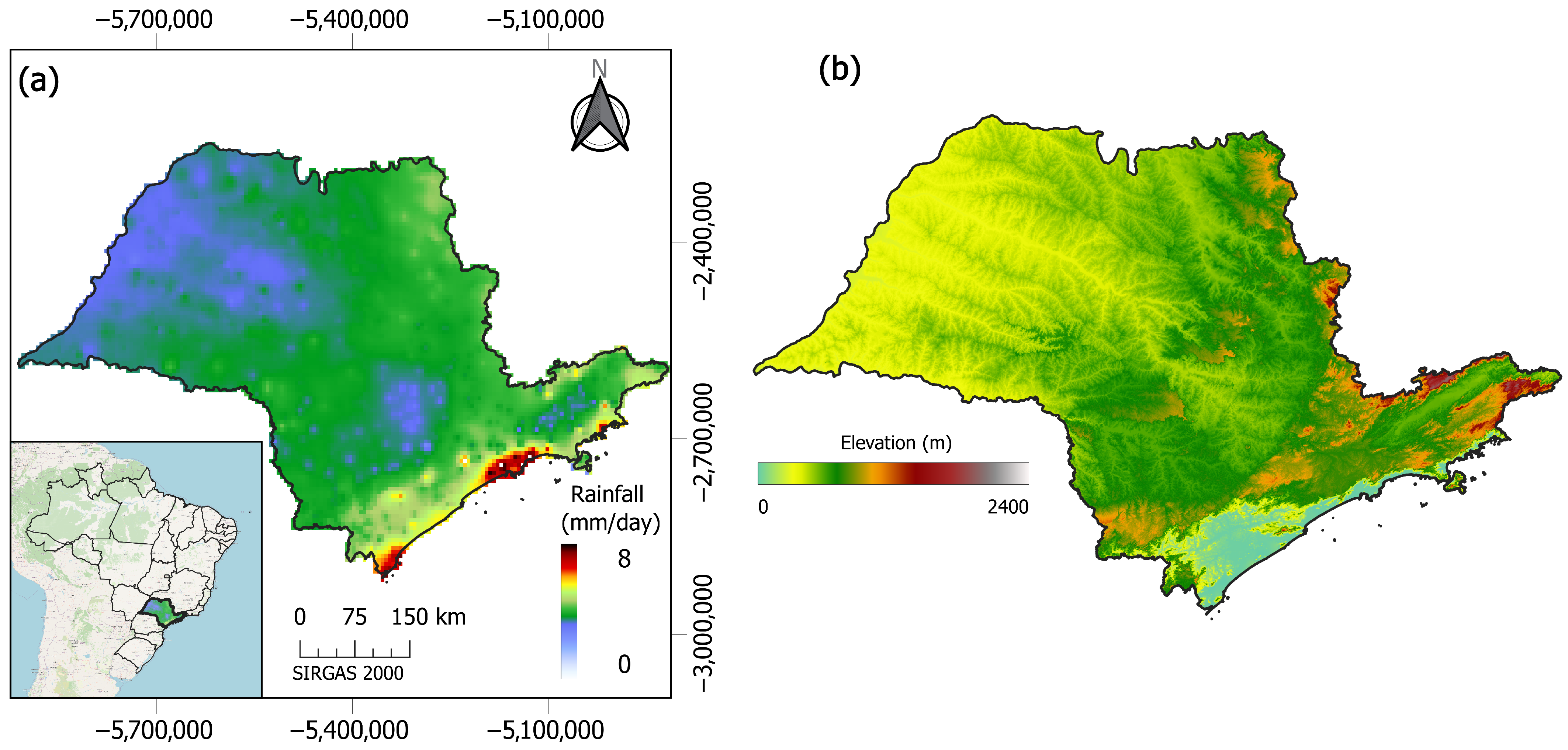
This study focuses on the São Paulo State, located in the Southeast region of Brazil (Figure 1). The state covers approximately 248,000 km² and comprises 645 municipalities. With about 46 million inhabitants according to the 2022 census [40], São Paulo is the most populous Brazilian state, housing roughly 22% of the national population. The study region is predominantly characterized by a humid subtropical regime (Cwa in the Köppen classification); [41]), with warm, wet summers and milder, drier winters. Mean annual rainfall is about 1400–1500 mm, with strong seasonality: most rainfall occurs during the austral summer (December–February), while the winter months (June–August) are comparatively dry.

To assess the temporal evolution and spatial distribution of flood-related events across municipalities in the São Paulo State, we used records from the Digital Atlas of Disasters in Brazil, an official database maintained by the Brazilian Ministry of Regional Development through the National Secretariat for Protection and Civil Defense [44]. The Atlas compiles municipal-level disaster records reported since 1991, including information on event type, year of occurrence, and affected locations. For this study, we extracted all records between 1991 and 2024 associated with flood-related processes, using the following event categories and keywords: flood, flash flood, urban flooding, river overflow, and inundation (hereafter referred to as ‘floods’). These data supported the characterization of growth and spatial heterogeneity in flood occurrence across São Paulo municipalities and to provide an empirical basis for linking observed impacts to projected changes in design rainfall and infrastructure requirements.

To represent climate variability and change in rainfall, we used the Climate Change Dataset for Brazil (CLIMBra; [45]), which provides an ensemble of 19 bias-corrected CMIP6 climate projections for Brazil. CLIMBra includes historical simulations (1980–2013) and future projections (2015–2100) at 0.25° × 0.25° spatial resolution for two Shared Socioeconomic Pathway (SSP) scenarios: SSP2-4.5 (intermediate) and SSP5-8.5 (upper bound). In the dataset, daily time series of rainfall were bias-corrected using the Quantile Delta Mapping (QDM) approach [46]. Here, we used an updated version of CLIMBra’s rainfall data, in which climate projections are bias-corrected using MSWEP-based observational data [47] rather than the dataset of Xavier et al. [48], due to its superior performance in representing the right-tail distribution of rainfall events.

For each grid cell and analysis period, annual maximum daily rainfall was extracted and fitted with a Generalized Extreme Value (GEV) distribution to estimate design rainfall depths for RP of 2, 10, 25, 50, and 100 years. The GEV distribution was adopted as the primary tail model because it provides a flexible extreme-value framework and has been identified as an adequate model for extreme rainfall in São Paulo State based on combined predictive and descriptive diagnostics [49]. To verify suitability for this dataset, a Monte Carlo goodness-of-fit evaluation assessed model performance: the evaluation generated synthetic samples from the fitted GEV distribution, and the observed Kolmogorov–Smirnov statistic and return levels across RPs fell within the 95% Monte Carlo confidence envelopes, supporting model adequacy. For comparability with Brazilian engineering practice, we also fitted the Gumbel distribution as a benchmark, since it is widely used in national manuals and technical workflows for drainage design. A quantitative comparison between GEV and Gumbel estimates is reported in the Supplementary Materials (Figures S1 and S2), showing that differences in design rainfall are modest for the return periods most relevant to culvert design (e.g., typically <5% for RP = 25 years and generally <10% for RP = 100 years across the study region). All projected design rainfall values and all subsequent impact calculations in this study rely on the GEV fits; the Gumbel results serve only as a sensitivity analysis to document the influence of tail-model choice relative to the larger spread among CMIP6 climate projections.

The analysis then aggregated the resulting gridded design rainfall depths (i.e., grid-cell return levels) to the municipal scale using area-weighted means based on their intersection with municipal boundaries. We compared design rainfall depths between the baseline period (1980–2013) and two future windows: immediate future (2015–2055) and distant future (2056–2100), for both SSP2-4.5 and SSP5-8.5. This approach to incorporating climate change effects on rainfall is consistent with the methodology adopted in most (91%) of studies reported in the literature [25].

Although temporal changes in extreme rainfall have been widely documented, the use of explicitly nonstationary frequency models remains debated, particularly when no clear physical relationship between distribution parameters and external covariates can be established [49,50,51,52]. In this study, frequency analyses were therefore conducted separately for historical, immediate-future, and distant-future periods rather than using a fully time-varying model. This time-slice approach preserves the projected climate change signal in each period while maintaining consistency with current engineering design practice. Consistently, the analysis also generated bias-corrected climate projections separately for the immediate and distant future periods, ensuring that the rainfall series used in the frequency analysis explicitly represent distinct change signals.

2.2. Discharge Project

To isolate and explore the effect of nonstationary rainfall on design discharge resulting implications for infrastructure sizing and costs, we adopted standardized, hypothetical catchments for all municipalities in the São Paulo State. This approach avoids confounding effects associated with local differences in catchment morphometry and land-surface characteristics and supports the interpretation of the results primarily as a climate-driven signal. By imposing a common hydrological configuration across all locations, the analysis enables a consistent comparison of how changes in rainfall regimes alone affect design and cost metrics.

This modeling chain is consistent with established approaches in the stormwater design literature. Climate-informed studies commonly employ hypothetical or standardized catchments to isolate climate effects from local catchment characteristics, update IDF relationships, propagate them through simplified rainfall–runoff transformations, and subsequently map the resulting design flows onto discrete, commercially available conduit or culvert classes, yielding stepwise changes in nominal size and associated costs (e.g., [29,53,54]). Our analysis follows the same structure to ensure comparability with previous studies. Nevertheless, the results should be interpreted as a first-order, climate-driven signal, rather than as representations of actual municipal drainage conditions.

Hydrological computations were performed for urban catchments with drainage areas A = 3, 125, and 250 km², spanning a representative range used in the development and application of the Natural Resources Conservation Service Curve Number (NRCS-CN) methodology [55,56]. Although the practitioners have applied the NRCS-CN method to much larger catchments, these areas are consistent with its conceptual basis and practical engineering use. To represent a broad spectrum of land-use and imperviousness conditions, we tested CN = 50, 75, and 98, covering conditions from less urbanized to highly impervious catchments. This range is consistent with commonly reported design values, with only rare exceptions outside this interval [55].

Runoff production was estimated using the NRCS-CN rainfall–runoff relationship:

$$Q(P)=\{\begin{array}{c}0, P\le \mathsf{\lambda }S\\ {\displaystyle \frac{(P-\mathsf{\lambda }S)}{P+(1-\mathsf{\lambda })S}} , P>\mathsf{\lambda }S\end{array} \}$$

(1)

where $Q$ represents the effective rainfall depth (mm), $P$ is rainfall depth (mm), $S$ is the potential maximum capacity storage (mm), and λ is the initial abstraction ratio (dimensionless). The capacity storage $S$ is given by:

$$S={\displaystyle \frac{\mathrm{25,400}}{CN}}-254$$

(2)

where $CN$ is the curve number (dimensionless).

Following recent empirical evidence showing improved performance relative to the traditional value of λ = 0.20, we adopted λ = 0.05, consistent with recent studies across different climatic regions and urban contexts [57,58,59,60,61] and with updates incorporated into current NRCS guidance [62].

Design rainfall depths were derived for durations $D$ = 1 h, 6 h, and 24 h, selected to span typical concentration-time ranges from small to medium catchments and to provide a longer-duration proxy relevant to larger catchments [29,53,63]. Because the climate projections used in this study provide rainfall at daily resolution, sub-daily design rainfall depths were obtained through temporal disaggregation of 24-h totals. Rather than adopting a single constant reduction factor, as commonly done in Brazil’s engineering practices, we employed spatially variable duration-reduction factors defined at the municipal level. We derived duration-reduction factors from observation-based gridded IDF information for Brazil (GRIDF-BR; [64]), which provides an updated, spatially explicit version of the duration-reduction factors originally recommended by the Environmental Company of the State of São Paulo [56]. This procedure accounts for the present-day spatial variability in rainfall temporal structure across the study region and reflects common practice when sub-daily climate or local IDF curves are unavailable (see Supplementary Figure S3 for the spatial patterns of coefficients adopted).

Nevertheless, these reduction factors rely on historical observations and implicitly assume a stationary intra-event rainfall structure. Potential climate change-induced modifications in sub-daily rainfall characteristics, such as increased convective contribution, shorter effective durations, or enhanced intensity concentration, cannot be explicitly resolved with daily climate data. Therefore, sub-daily design results remain conditional on the adopted duration-reduction factors.

The analysis subsequently used the resulting effective rainfall depth $Q$ for each municipality and RP to estimate the design peak discharge using the NRCS-CN unit hydrograph approach, assuming the standard triangular dimensionless unit hydrograph formulation. Consistent with common design practice, we adopted a critical-duration assumption in which the rainfall duration is taken approximately equal to the catchment response time ($T_c$). Accordingly, for each evaluated rainfall duration ($D$ = 1 h, 6 h, and 24 h), we set the time of concentration equal to the rainfall duration ($T_c$ = $D$), while the lag time ($T_{lag}$) was derived using the NRCS empirical relation (Equation (3))

$$T_{lag}=0.6·T_c$$

(3)

and the time to peak $T_p$ as

$$T_p={\displaystyle \frac{D}{2}}+T_{lag}$$

(4)

where $T_c$ is the catchment time of concentration (hours), $T_{lag}$ is the catchment lag time (hours), $D$ is the duration of the rainfall (hours), and $T_p$ is the time to peak (hours).

Under these assumptions, the peak discharge $Q_p$ (m³·s⁻¹) associated with the total effective rainfall $Q$ (mm) was estimated using the standard NRCS unit hydrograph:

$$Q_p={\displaystyle \frac{0.208·A·Q}{T_p}}$$

(5)

where $Q_p$ is the peak discharge (m³·s⁻¹), A is the catchment area (km²), $Q$ is the effective rainfall depth (mm), and $T_p$ is the time to peak (hours).

2.3. Culvert Design Example

To evaluate the potential impacts of climate change on urban drainage infrastructure, we used culverts as they are widely used in engineering practice, occur in a variety of settings, and typically account for a substantial share of drainage-related construction costs when compared with smaller elements such as inlets or gutters. Culvert design is generally associated with relatively frequent events (RP ≤ 100 years). At longer RP, other interventions, including larger underground galleries, short-span bridges, or small bridge structures, are often more appropriate from both technical and economic perspectives. Additionally, limiting the analysis to RP ≤ 100 years reduces excessive extrapolation beyond the observational record.

Hydraulic sizing and capacity checks follow Brazilian design practice and the formulations in Brazilian National Department of Transport Infrastructure [65] and Baptista and Coelho [66] (Equations (7) and (8)), unless stated otherwise.

$$Q={\displaystyle \frac{1}{n}}{A}_m{R_h}^{2/3}{I_0}^{1/2}$$

(6)

where $Q$ is discharge (m³·s⁻¹), $A_m$ is the cross-sectional flow area (m²), $R_h$ is the hydraulic radius ($m$), $I_0$ the barrel slope ($\mathrm{m}·{\mathrm{m}}^{-1}$), and $n$ is Manning–Strickler’s roughness coefficient ($\mathrm{s}·{\mathrm{m}}^{-1/3})$.

The design peak discharges obtained from the hydrological analysis were then used to dimension square concrete box-culvert cells, considering commercially typical culvert sizes available in Brazil, where B is the cell width and H is the cell height, with $B=H \in \{1.0, 1.5, 2.0, 2.5, 3.0, 3.5, 4.0\}$ m, ensuring that reported dimensions and costs correspond to implementable designs. The longitudinal slope of the culvert barrel was fixed at 0.01, and the Manning roughness coefficient was set to 0.015. For hydraulic-based assessments, the culvert length was fixed at 1 m, so that results can be interpreted on a per–linear-meter basis.

The design allowed multiple parallel barrel lines without a priori upper limit (in practice, the number of lines would be constrained by the right-of-way and local site conditions). The analysis considered parallel barrels only when a single barrel could not convey the design discharge for a given RP. To account for hydraulic interaction between adjacent barrels, a conservative, empirical reduction of 5% was applied for each additional line beyond the first. For each candidate configuration (number of lines × nominal cell size), conveyance capacity was estimated under an idealized barrel-controlled assumption based on the expected internal-flow regime. Inlet control and local head losses (entrance/exit and approach losses) were not explicitly modeled; therefore, reported sizes and costs should be interpreted as screening-level, lower bound estimates that may increase where inlet control or headwater effects are significant.

For each candidate box size, the critical slope ($I_c$) was computed using the following expression:

$$I_c=\left({\displaystyle \frac{2.6n^2}{\sqrt[3]{H}}}\right){\left(3+{\displaystyle \frac{4H}{B}}\right)}^{4/3}$$

(7)

where $I_c$ is the critical slope (m/m), $n$ is Manning–Strickler’s roughness coefficient ($s·{\mathrm{m}}^{-1/3})$, $H$ is the internal culvert height (m), and $B$ is the internal culvert width (m).

If the actual barrel slope $I_0$ was smaller than $I_c$, the flow was assumed to be subcritical, and the subcritical capacity formula was used. Otherwise, a supercritical capacity formula was adopted. In both cases, an effective flow depth of $0.8H$ (i.e., a 20% freeboard) was assumed. Under subcritical conditions ($I_0$ < $I_c$), the unit capacity per cell $\left(Q_{adm, subcrit}\right)$ was estimated using a formula derived from Manning-type relationships for rectangular culverts:

$$Q_{adm, subcrit}={\left[{\displaystyle \frac{{\left(0.8BH\right)}^5}{{\left(B+1.6H\right)}^2}}\right]}^{1/3}{\displaystyle \frac{{I_0}^{1/2}}{n}}$$

(8)

where $Q_{adm, subcrit}$ is the admissible unit discharge capacity per cell under subcritical conditions (m³·s⁻¹), $I_0$ is the barrel slope ($\mathrm{m}·{\mathrm{m}}^{-1}$), $n$ is Manning–Strickler’s roughness coefficient ($\mathrm{s}·{\mathrm{m}}^{-1/3})$, $H$ is the internal culvert height (m), and $B$ is the internal culvert width (m).

For supercritical conditions ($I_0$ ≥ $I_c$), a simplified empirical relationship was adopted for the unit capacity per cell:

$$Q_{adm, supcrit}=1.705B{H}^{3/2}$$

(9)

where $Q_{adm, supcrit}$ is the admissible unit discharge capacity per cell under supercritical conditions (m³·s⁻¹), $H$ is the internal culvert height (m), and $B$ is the internal culvert width (m).

2.4. Costs of Constructions

Estimated construction costs depend strongly on project location, site-specific constraints, and procurement conditions. Because this study is based on a hypothetical site and aims at a comparative, scenario-based assessment of climate change impacts on infrastructure costs, we adopted a simplified and standardized cost framework suitable for first-order analysis. Accordingly, a representative set of typical services for small culvert projects was defined (Table S1, in the Supplementary File), and all costs were expressed per linear meter of culvert barrel, following standard public-works practice in Brazil.

Unit prices came from three official Brazilian public cost databases. The primary source was the National System of Construction Costs and Indexes—SINAPI [67], which is the standard reference database for preliminary cost estimates in Brazilian public works, which is widely used for budgeting and tendering purposes. When specific culvert-related services were not available or were not insufficiently represented in SINAPI, unit prices were complemented using other officially recognized databases, namely the Federal Highway Works Cost System—SICRO [68] and the São Paulo Municipal Urban Infrastructure Cost System—SIURB [69], following common engineering practice in Brazil.

In addition to direct construction costs, project budgets must account for indirect costs, overheads, and contractor profit. In Brazilian public works, practitioners commonly aggregate these components into a single mark-up factor known as the BDI (“Budget Difference Index”). In this study, we adopted the non–payroll-tax-relief configuration and followed the baseline formulation recommended by the Brazilian Federal Court of Audit—TCU [70] for service contracts. Accordingly, a uniform BDI factor of 21.33% was applied to all direct costs (Table S2, in the Supplementary File), yielding total construction costs inclusive of overheads and profit, as illustrated in the example bill of quantities (Table S2, in the Supplementary File). This value falls within the typical range recommended by TCU, while acknowledging that actual contract prices may vary depending on project-specific negotiations and market conditions.

3. Results and Discussion

3.1. Temporal Evolution of Extreme Rainfall Events in São Paulo State

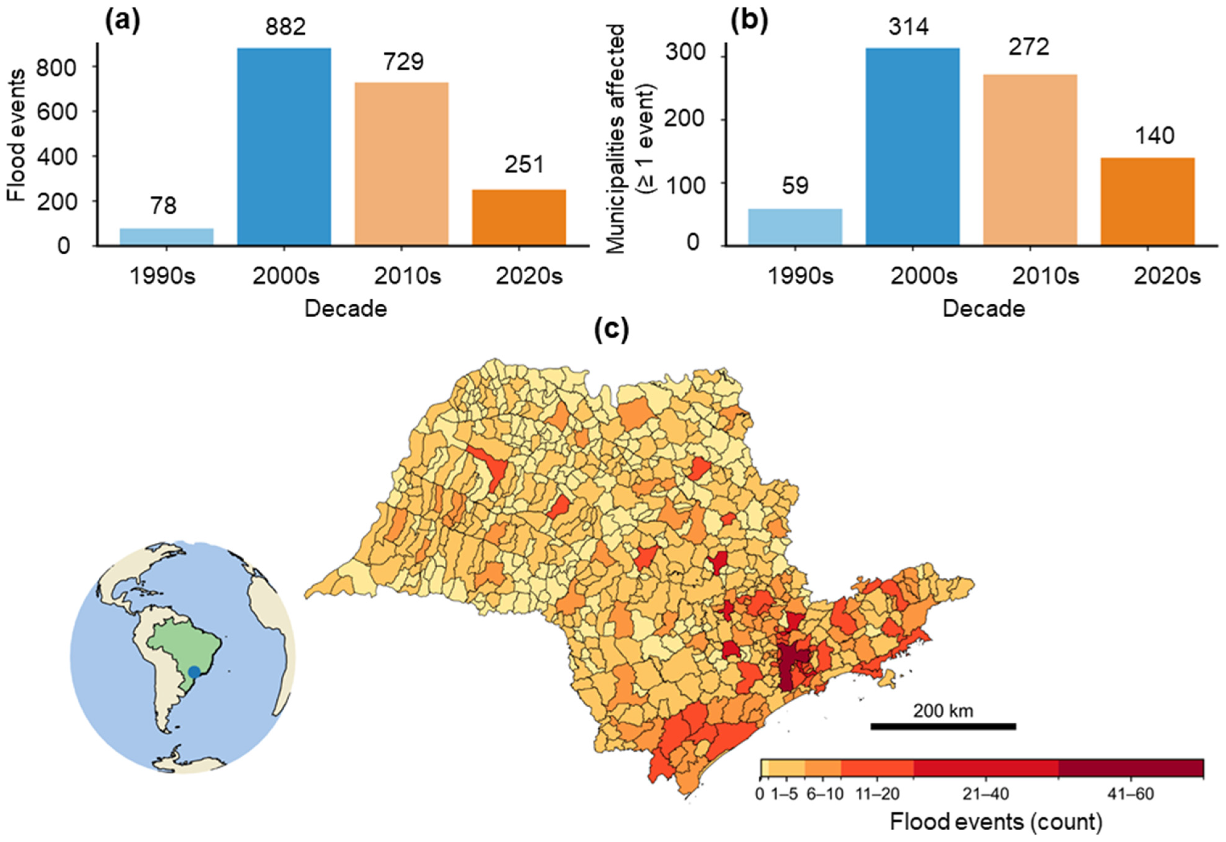
As São Paulo State is a major economic hub in Brazil, understanding its climatic and hydrological dynamics is critical for maintaining the continuity of economic activity and essential services. Floods can generate welfare and competitiveness losses that propagate beyond municipal boundaries [37]. In this context, a marked intensification of flood occurrence has been observed over recent decades. The total number of events increased sharply from 78 in the 1990s to 882 in the 2000s (+1030%; Figure 2a). Although a slight decrease is observed in the 2010s (729 events, i.e., 73 events per year) and in the early 2020s (251 events, noting that the period from 2020 to 2024 does not represent a full decade), events count remains substantially higher than those recorded in the 1990s. The number of municipalities reporting at least one flood-related event increased from 59 in the 1990s to a peak of 314 in the 2000s (approximately 48% of the state’s municipalities), followed by a moderate reduction in the 2010s (272) and in the early 2020s (140) (Figure 2b).

Eastern São Paulo concentrates flood occurrence, especially the São Paulo Metropolitan Region, the coastal zone, and the Paraíba Valley, where several municipalities recorded more than 20 events over the last four decades (Figure 2c). In São Paulo city, for a 100 m impact radius, Haddad and Teixeira [37] estimate R$43.54 million in direct losses, translating into R$218.19 million in total losses at the national scale (impact–damage ratio = 5.0), with expected reductions of 0.0263% in the city’s Gross Regional Product (GRP) and 0.0071% in Brazil’s Gross Domestic Product (GDP). In contrast, much of the western and northwestern interior shows lower event frequencies, with many municipalities reporting fewer than 10 events. This spatial pattern suggests that the increase in flood occurrence increased through both higher frequency and broader geographic coverage across the state.

Importantly, trends in human impacts do not mirror the temporal evolution of event counts. In parallel with the intensification of flood occurrence—and beyond direct economic losses—indicators of human impact increased markedly, suggesting an amplification driven by growing exposure and vulnerability [44]. The number of displaced and homeless individuals increased from the 1990s (25.54 thousand) to the 2000s (113.31 thousand), and reached its maximum in the 2010s (178.07 thousand), despite a reduction in the total number of recorded flood events relative to the previous decade. Injured and ill individuals follow the same pattern, increasing from 234 in the 1990s to 4710 in the 2010s.

Although the numbers for 2020–2024 are not directly comparable to full decades, the 48.49 thousand displaced and homeless individuals recorded in only five years indicate that high-severity impacts continue to recur. These results suggest that, while flood frequency peaked in the 2000s, the severity of impacts on populations intensified into the 2010s, consistent with increasing exposure and vulnerability across the state.

From a hydrological and climatic perspective, these results reinforce that isolated increases in rainfall alone do not explain the intensification of flood impacts. Previous studies showed that changes in these variables alone do not explain the occurrence of extreme events [32,33]. In São Paulo State, the observed impacts emerge from the interaction between climatic forcing and characteristics of the river basin and urban system. Evidence indicates a significant increase in total annual rainfall and in the frequency of intense events (≥20 mm and ≥100 mm), particularly during summer, concomitant with an increase in the number of consecutive dry days [71,72]. This reorganization of the rainfall regime, together with the modulation of runoff by catchment state and structure, and the combined effects of hazard, exposure, and infrastructure limitations, could favor rapid hydrological responses and amplifies flood risk, particularly in densely urbanized and hydrologically modified catchments such as the São Paulo Metropolitan Region.

3.2. Design Discharge Response Across Return Periods

This study examines how construction costs and culvert dimensions vary across five RPs (RP ≤ 100 years) under a nonstationary rainfall, i.e., under the effects of climate change in the state of São Paulo. To interpret the resulting design discharge ($\mathsf{\Delta }\mathrm{Q}$) and cross-sectional area ($\mathsf{\Delta }\mathrm{A}$) signals, it is important to acknowledge that event-based urban design practice still relies on simplified rainfall–runoff methods (e.g., Rational, Simple, Santa Barbara Urban Hydrograph) because of their low data requirements and transparency, but these methods introduce structural uncertainty through strong assumptions about runoff generation and routing that are not universally valid [63]. Comparative evaluations indicate that NRCS-CN-based formulations can provide more reliable runoff response across a broader range of conditions than single-coefficient approaches, supporting their use as a pragmatic benchmark for design sensitivity studies [60,63]. In particular, prior studies indicate that NRCS-CN-based approaches can be appropriate for culvert design contexts, where peak discharge sensitivity to effective runoff generation is central [73].

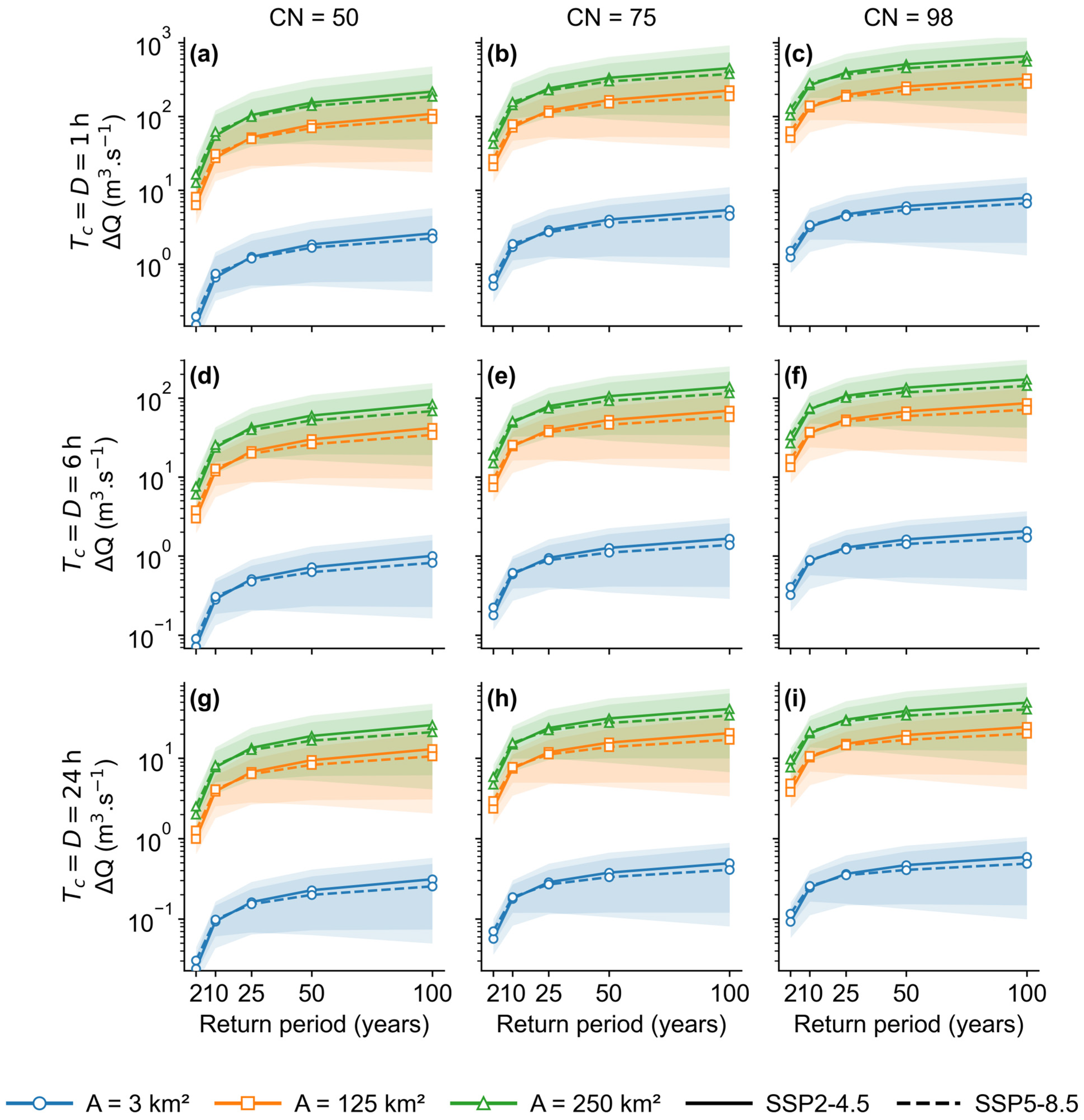
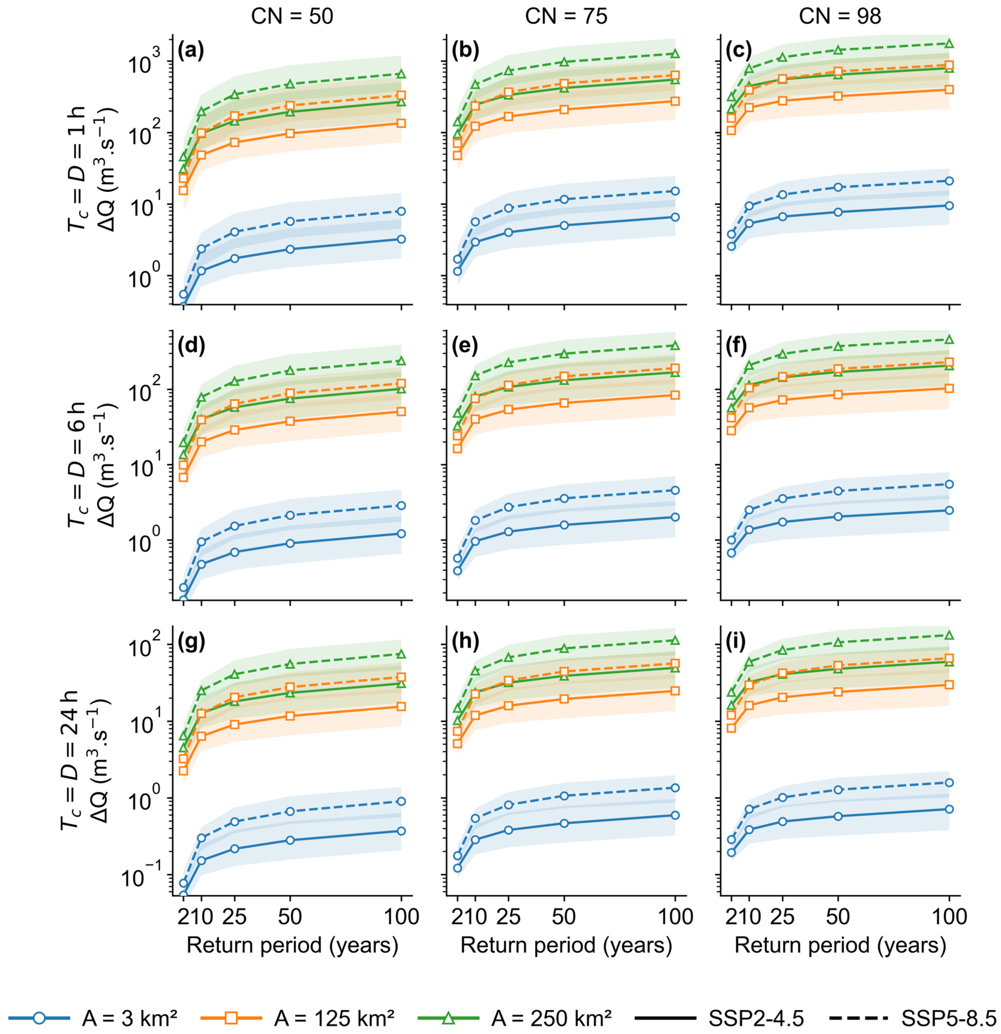
We analyze how nonstationary changes in propagate into coupled changes in design discharge ($\mathsf{\Delta }\mathrm{Q}$) and cross-sectional area $\left(\mathsf{\Delta }\mathrm{A}\right)$, and consequently into culvert conveyance capacity and sizing. The assessment was conducted through a factorial experiment combining three $\mathrm{C}\mathrm{N}$ levels (50, 75, and 98), three areas (3, 125, and 250 km²), and three design durations (${\mathrm{T}}_{\mathrm{c}}$ = D = 1, 6, and 24 h), under SSP2-4.5 and SSP5-8.5 scenarios, for the immediate future (2015–2055) and distant future (2056–2100), both referenced to the historical baseline (1980–2013). Figure 3 and Figure 4 summarize $\mathsf{\Delta }\mathrm{Q}$ across return periods, showing that $\mathsf{\Delta }\mathrm{Q}$ generally increases under both scenarios and that the distant-future signal is typically stronger than the immediate-future signal, with differences between futures horizons reaching up to a factor of three.

Across both horizons, $\mathsf{\Delta }\mathrm{Q}$ exhibits a monotonic response to design parameters: it increases with catchment area, $\mathrm{C}\mathrm{N}$, and $\mathrm{R}\mathrm{P}$, and decreases with increasing duration (Figure 3 and Figure 4). In terms of sensitivity ranking, area and duration dominate the absolute discharge response, consistent with studies finding that rainfall intensity and contributing area are primary controls of peak runoff in event-based design [60]. Increasing the contributing area by two orders of magnitude (from 3 km² to 250 km²) produces increases of tens of times. In contrast, extending the duration from 1 h to 24 h reduces $\mathsf{\Delta }\mathrm{Q}$ by roughly one order of magnitude (about an 8–14-fold decrease), in cases with high CN and $\mathrm{R}\mathrm{P}$. This behavior is consistent with the design logic of event-based rainfall–runoff methods, in which short design durations concentrate rainfall intensity and therefore control peak discharge. The magnitude of this effect depends on runoff-production assumptions (i.e., initial abstraction ratio in CN-based formulations), and it highlights that equating the critical duration to the catchment response time concentration can be restrictive in heterogeneous catchments and under nonstationary climates [58,63].

Changes in CN and RP act as secondary, though still relevant, amplifiers. Increasing RP from frequent to rarer events typically multiplies median $\mathsf{\Delta }\mathrm{Q}$ by about 4–17 times, while higher CN values systematically increase $\mathsf{\Delta }\mathrm{Q}$, especially when combined with larger areas and shorter durations. For instance, for A = 125 km², T_c = 1 h, and CN = 50 (SSP2-4.5), increasing RP from 2 to 100 years raises $\mathsf{\Delta }\mathrm{Q}$ by approximately 6 times; under the same conditions and RP = 100, increasing CN from 50 to 98 increases ΔQ by about 3 times. A comparison between scenarios shows that, in the immediate future, SSP2-4.5 and SSP5-8.5 curves generally remain closely paired, indicating that sensitivity to hydrological and geometric parameters (A, CN, RP, and T_c = D) dominates the signal. In the distant future, however, SSP5-8.5 tends to exhibit a more persistent upward shift, making inter-scenario differences more evident and in some cases larger than in the immediate future, depending on the parameter combination (e.g., RP = 2, CN = 98, A = 3 km², D = 1 h, with an average difference of about 48% between SSPs). Nevertheless, spatial dispersion (10th–90th) remains wide across both scenarios and horizons, increasing with return period. This reflects heterogeneity among municipalities associated with differences in the projected rainfall-change signal across climate models, even under standardized hydrological configurations. The stronger dispersion and scenario separation for rarer events is consistent with evidence that flood response under warming depends on event rarity and on how extremes scale with thermodynamic and circulation changes [32] and reinforces the broader point that neglecting nonstationarity and deep uncertainty can underestimate flood risk and bias infrastructure decisions [2,11].

In design practice, engineers often translate climate-change signals into uplift factors for extreme rainfall or design flows, commonly on the order of 20–40% in European, Oceania, and North American guidance (e.g., [15,17,27,29,74,75,76,77]). In Brazil, recent national-level guidance has addressed climate-change impacts on water resources in broader terms [78], but drainage-specific standards translating climate change into explicit design requirements remain limited. The closest analogue is the post-event technical note by Paiva et al. [16], produced in the context of the 2023–2024 extreme events in southern Brazil [79], which suggests 15% increases for RP ≤ 10 years and 20% for higher return periods. Against this benchmark, our projected $\mathsf{\Delta }\mathrm{Q}$ broadly overlaps with these allowance ranges, but the distributions reveal heterogeneity across municipalities and scenarios. For T_c = D = 1 h in the immediate future (Figure 3), SSP2-4.5 medians reach 26–43% for CN = 50 and 16–28% for CN = 75, whereas CN = 98 yields smaller increases (9–16%), broadly comparable in order of magnitude to the 15–20% proposal under highly impervious conditions. Under SSP5-8.5, the distributions shift upward (medians 35–42%, 20–28% and 11–16% for CN = 50, 75 and 98, respectively), and upper tails commonly exceed “classical” allowances, indicating that a single factor can be conservative for some municipalities and insufficient for others.

This spread reflects two structural features of the problem. First,$\mathsf{\Delta }\mathrm{Q}$ remains largely insensitive to drainage area in our factorial framework; area mainly rescales absolute discharges, while the dependence on CN persists. Lower CN tends to yield larger fractional changes, consistent with nonlinear runoff generation and the sensitivity of effective excess to intensified extremes. Second, simplified event-based methods embed strong loss representations; single-coefficient approaches such as the Rational method, although operationally attractive, may underestimate peak discharge when infiltration and nonlinear losses are oversimplified, particularly under heterogeneous catchment conditions [60,63]. Together, these points help explain why uniform uplift factors may not transfer reliably across hydrologic regimes: allowances that align with impervious settings can underestimate relative changes under more permeable conditions, especially as SSP5-8.5 amplifies upper-tail responses. The stronger SSP5-8.5 upper-tail response is physically consistent with CC thermodynamic scaling, which sets an expected intensification of short-duration extremes under warming and tends to be larger for rarer events [23]. Yet deviations from simple CC scaling arise because large-scale atmospheric dynamics and temporal-scale dependence modulate extremes, helping explain the persistent spread in results [20].

3.3. Nominal-Section Upgrades and Required Area Changes

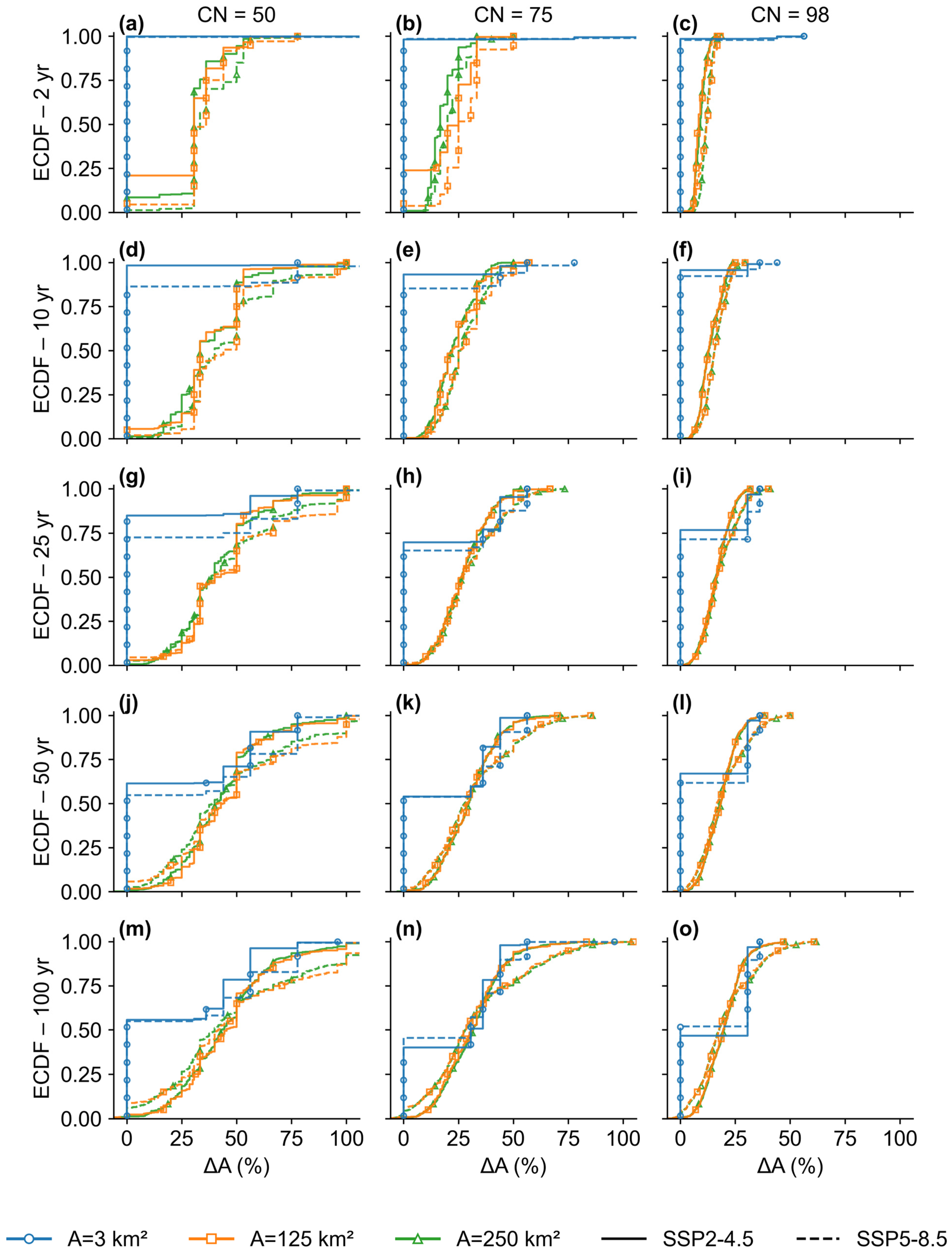
To translate projected design-discharge changes into actionable infrastructure implications, we report the relative changes in effective culvert section area ($\mathsf{\Delta }\mathrm{A}$) after mapping the hydraulically required area to commercially available nominal-section classes. This choice reflects field practice, where designs and retrofits typically adopt the next available nominal size rather than a continuously varying area. A direct consequence is that $\mathsf{\Delta }\mathrm{A}$ becomes a discretized variable, so the empirical cumulative distribution functions (ECDFs) exhibit step-like plateaus: municipalities may experience non-zero changes in design discharge while remaining within the same nominal class ($\mathsf{\Delta }\mathrm{A}=0$), whereas others shift to a higher class once a threshold is crossed. This motivates reporting $\mathrm{P}(\mathsf{\Delta }\mathrm{A}>0)$ as the fraction of municipalities that cross at least one nominal-size threshold, i.e., how many projects would require a section-class upgrade under the catalogue constraint.

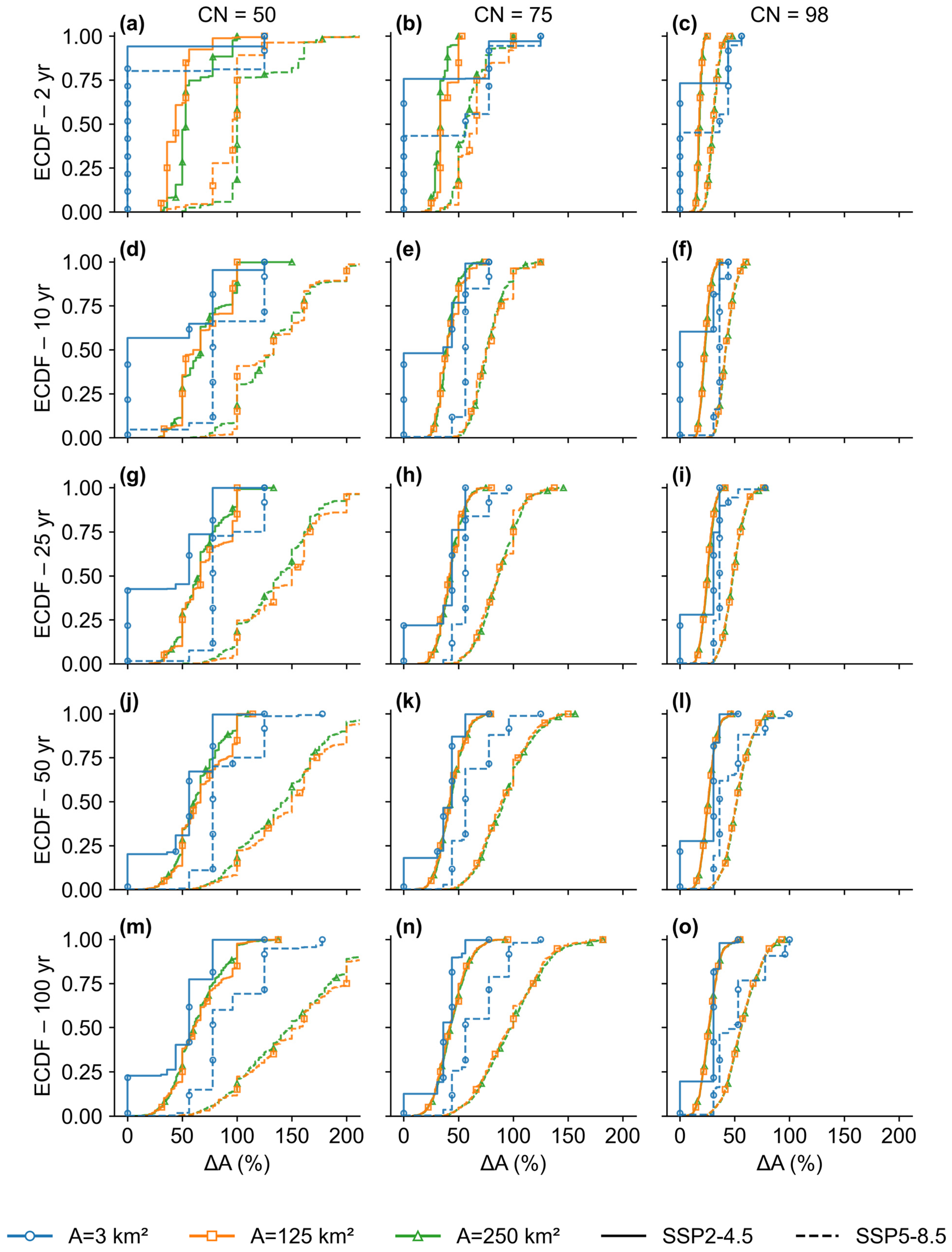
In the main text, we presents the results for a 1 h rainfall duration for both the immediate future (Figure 5) and the distant future (Figure 6). In the Supplementary Materials, Figures S4 and S5 correspond to the immediate future for other rainfall durations, while Figures S6 and S7 present the equivalent results for the distant future. Overall, the tendency toward larger required sections with increasing design discharge is similar across durations. The main difference is that, for larger catchments combined with shorter durations, percentage changes tend to be smaller than those observed when both catchment area and duration increase. This is physically consistent, since larger catchments generally have longer times of concentration; however, greater uncertainty is associated with applying the NRCS-CN method to large areas [55,57].

Differences between the immediate and distant future indicate a strong increase in the fraction of municipalities that exceed nominal-size thresholds, particularly in larger catchments. In the distant future, the influence of RP intensifies, leading to more frequent threshold crossings even in small catchments, as well as to larger step changes in section class, which in the immediate future often remained within the same nominal class. Responses are most sensitive under lower CN values, where the spread across municipalities is larger: section-area increases reach up to 100% in the immediate future and can approach 200% in the distant future. Higher CN values yield a more constrained range of outcomes.

In the immediate future, SSP2-4.5 and SSP5-8.5 yield largely overlapping results for most configurations, with clearer scenario differences limited to very small catchments, where SSP5-8.5 shows a more pronounced shift toward larger section increases. In the distant future, this SSP5-8.5 shift strengthens across all configurations. For example, for A = 250 km² and CN = 50, approximately 75% of municipalities exhibit increases up to 100% under SSP2-4.5 (Figure 6d), whereas under SSP5-8.5 the upper range extends to 160%. Drainage area strongly controls the likelihood of a nominal class change in the immediate future. For A = 125–250 km², $\mathrm{P}(\mathsf{\Delta }\mathrm{A}>0)$ is already high at low RP and rapidly approaches 100% for RP ≥ 10. However, for A = 3 km², most municipalities remain in the same class at RP = 2 ($\mathrm{P}(\mathsf{\Delta }\mathrm{A}>0)=0-2\mathrm{\%}$) and cross thresholds more frequently only as RP increases, reaching 44% under SSP2-4.5 and 45% under SSP5-8.5 at RP = 100. Overall, SSP5-8.5 systematically increases the fraction of municipalities exceeding section thresholds, particularly for smaller catchments. Differences associated with CN emerge primarily before saturation of $\mathrm{P}(\mathsf{\Delta }\mathrm{A}>0)$; because ΔA is discretized, local non-monotonic responses can occur, depending on a design’s position relative to catalogue step thresholds.

In the distant future, the threshold-crossing metric $\mathrm{P}(\mathsf{\Delta }\mathrm{A}>0)$ indicates a transition to a regime broadly dominated by nominal class changes. For A ≥ 125 km², $\mathrm{P}(\mathsf{\Delta }\mathrm{A}>0)$ reaches 100% across all scenarios, RPs, and CN values, suggesting that under the projected intensification of hydrologic extremes, all municipalities exceed at least one catalogue step. Discrimination among hydrologic combinations therefore occurs mainly for A = 3 km², where $\mathrm{P}(\mathsf{\Delta }\mathrm{A}>0)$ increases with RP and shows strong scenario sensitivity. At RP = 2, the fraction of municipalities changing section rises from still modest values under SSP2-4.5 (<6%) to substantially larger values under SSP5-8.5 (<20%). For RP ≥ 10, SSP5-8.5 approaches saturation even for small catchments, with approximately 43–95% of municipalities exhibiting a class change under SSP2-4.5 and SSP5-8.5, respectively. In addition, ΔA magnitudes increase in the distant future and shifted toward larger values under SSP5-8.5, consistent with the discretized nature of the variable, in which differences in design discharge manifest as jumps between nominal-section classes.

The dependence of projected discharge and section-area changes on RP reflects both climatic drivers and the rainfall–runoff transformation. In the Brazilian context, there is evidence that shifts in rainfall-event distributions are strongly controlled by changes in event frequency (in addition to intensity), which may particularly affect quantiles associated with shorter RP [31,72]. The dependence of projected cost changes on RP is also consistent with the nonlinear rainfall–runoff transformation embedded in the NRCS-CN method. In this formulation, direct runoff increases nonlinearly with effective rainfall; as a result, small changes in design rainfall can translate into disproportionately large relative changes in runoff for more frequent, lower-magnitude events, whereas for higher-intensity rainfalls the runoff response becomes nearly proportional to rainfall. This behavior can help explain the potential disagreement between projected changes across RP, particularly at shorter RP. In addition, evidence indicates that the initial abstraction ratio is not universal and that using values lower than the conventional 0.2 can substantially affect runoff estimates, particularly for lower rainfall depths or lower curve numbers [57,58,59,60,61,62], conditions that are more representative of shorter RP.

Finally, the selection of climate scenarios for design purposes involves uncertainties and prudential choices. SSP5-8.5 has been widely used as a high-emission reference and, in the short term, can serve as a useful benchmark for assessing risks under more severe conditions [11]. However, there are arguments that its late-century trajectory relies on unrealistic assumptions regarding continued fossil-fuel expansion [80]. Intermediate scenarios, such as SSP2-4.5, are sometimes considered overly optimistic by some authors, although they can be adopted as an alternative for analyses seeking a balance between plausibility and conservative design criteria [11,81,82].

3.4. Spatial Patterns of Cost Change

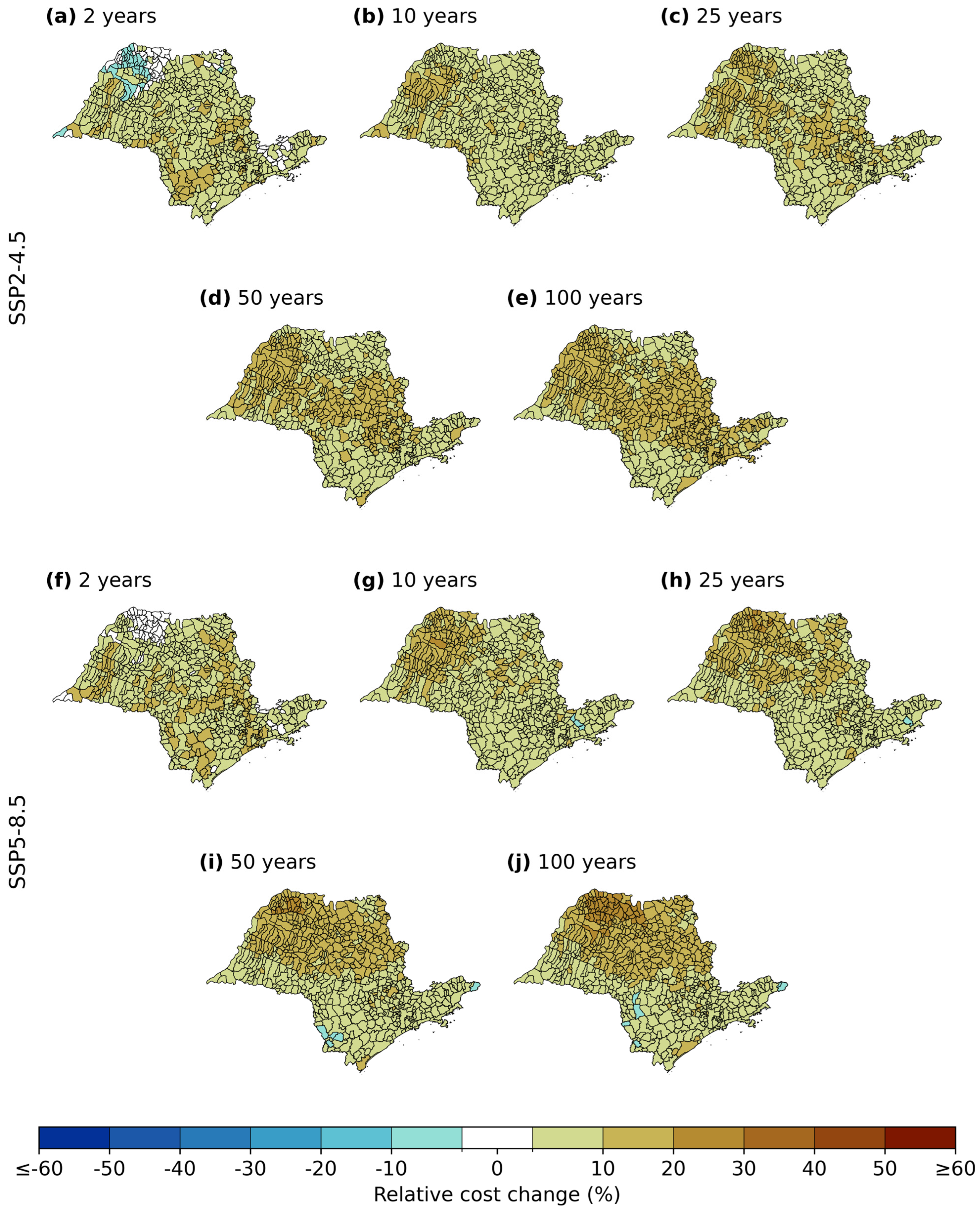
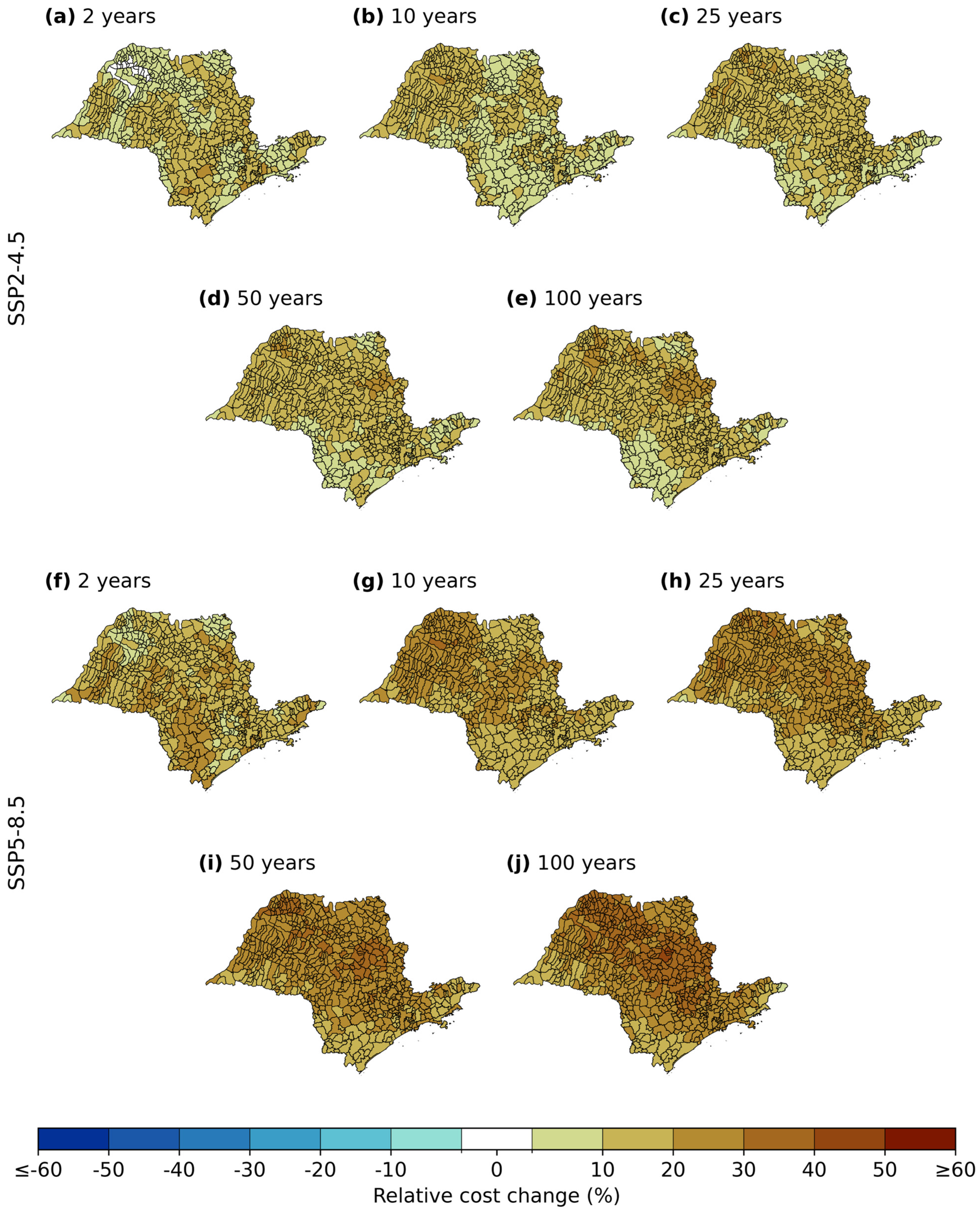
Relative construction-cost changes are mapped under a standardized, highly urbanized catchment configuration (CN = 98, A = 3 km², Tc = D = 1 h) to isolate climate-driven spatial variability across municipalities. Because culvert design uses discrete commercial sizes, the response exhibits threshold behavior: moderate increases in design discharge may remain within the same catalog class (no change in nominal diameter and cost), whereas exceedances trigger stepwise upgrades to the next section class and associated cost increases.

In the immediate future (2015–2055), projected relative changes in culvert construction costs show limited spatial variability across municipalities and RP (Figure 7). For RP up to 25 years, roughly 68% of municipalities show projected cost increases up to 10% under both the optimistic and pessimistic scenarios. For the remaining RP, this pattern persists under SSP2-4.5. Under SSP5-8.5, however, and for RP exceeding 25 years, about 46% of municipalities exceed 10% additional costs. These patterns are consistent with multi-model assessments reporting spatially heterogeneous but frequent substantial increases in design rainfall and extreme rainfall relevant to pluvial flooding, particularly for shorter-duration events that often control urban drainage design (e.g., [25,27,74]). Moreover, the observed increase in relative costs with RP is in line with studies reporting stronger climate-change-induced amplification of rainfall extremes associated with longer RPs, which directly translates into higher design discharges and more demanding infrastructure [30,31].

In the distant future (2056–2100), the ensemble indicates that projected changes intensify across São Paulo State (Figure 8). All municipalities continue to exhibit positive deviations in culvert construction costs relative to the baseline across all RPs and under both scenarios. For short RPs (≤25 years), relative cost changes increase, with approximately 86% of municipalities exceeding 10%. For longer RPs, both the spatial extent and the magnitude of changes increase further. Under SSP2-4.5, typical relative cost changes fall around 10–20% for 80% of municipalities, whereas under SSP5-8.5 the distribution shifts upward: for RP = 100 years, about 21% of municipalities cluster around 20–25%, and roughly 69% exceed 25%.

Figures S8, S9, S12, and S13 present variability analyses of projected relative changes in culvert construction costs and show the spread across the model ensemble. Overall, no-change outcomes dominate the lower tail of the distribution, mainly because discretization into commercially available section classes often keeps costs in the same category as the attach baseline. In contrast, the upper tail exhibits more substantial and spatially widespread increases, particularly under higher radiative forcing scenarios and over longer projection horizons. This pattern suggests that many municipalities still show conservative estimates at the lower end of the distribution, while more extreme projections increase the likelihood of significant cost escalation. These results underscore the importance of accounting for model-related uncertainty in infrastructure planning analyses.

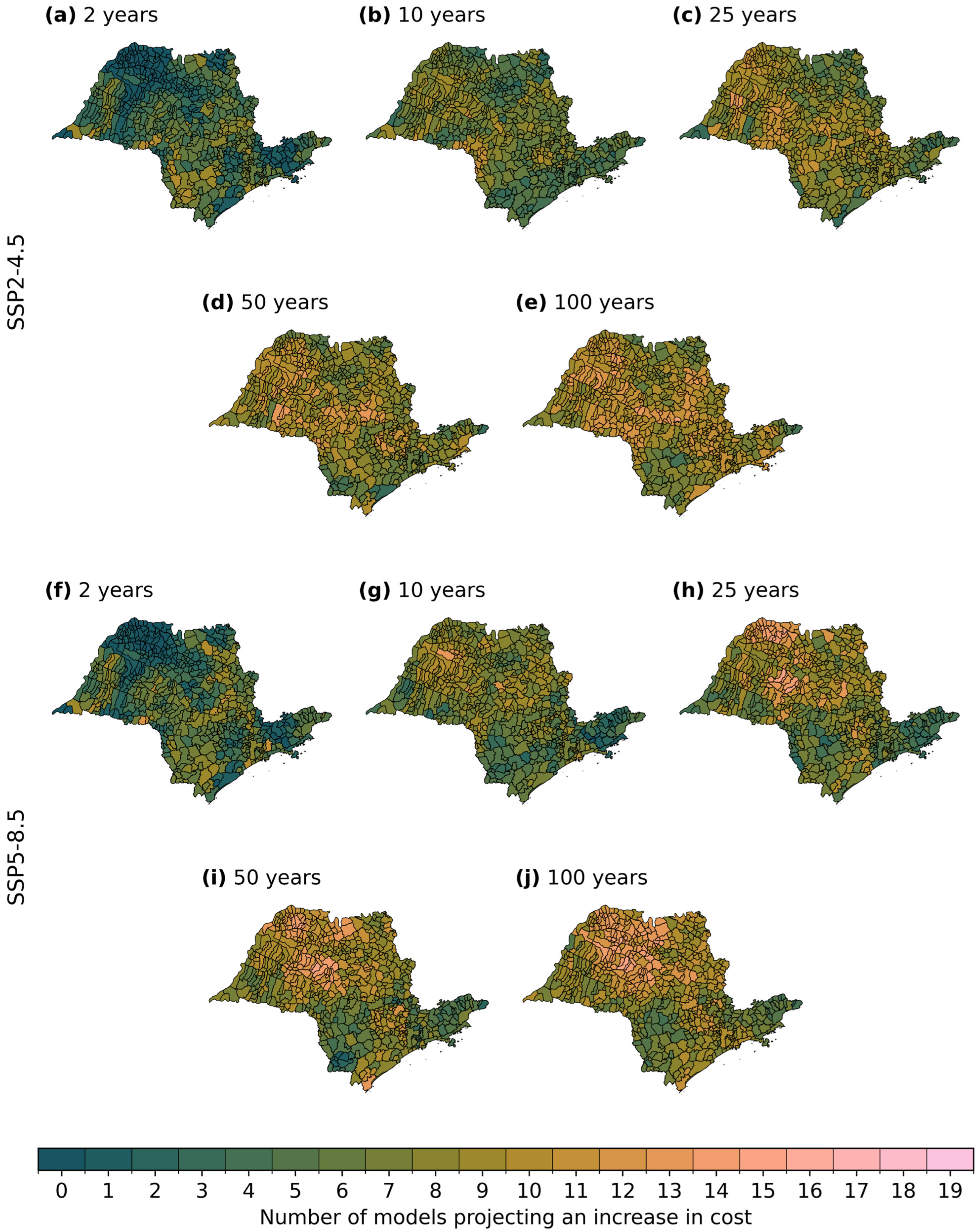
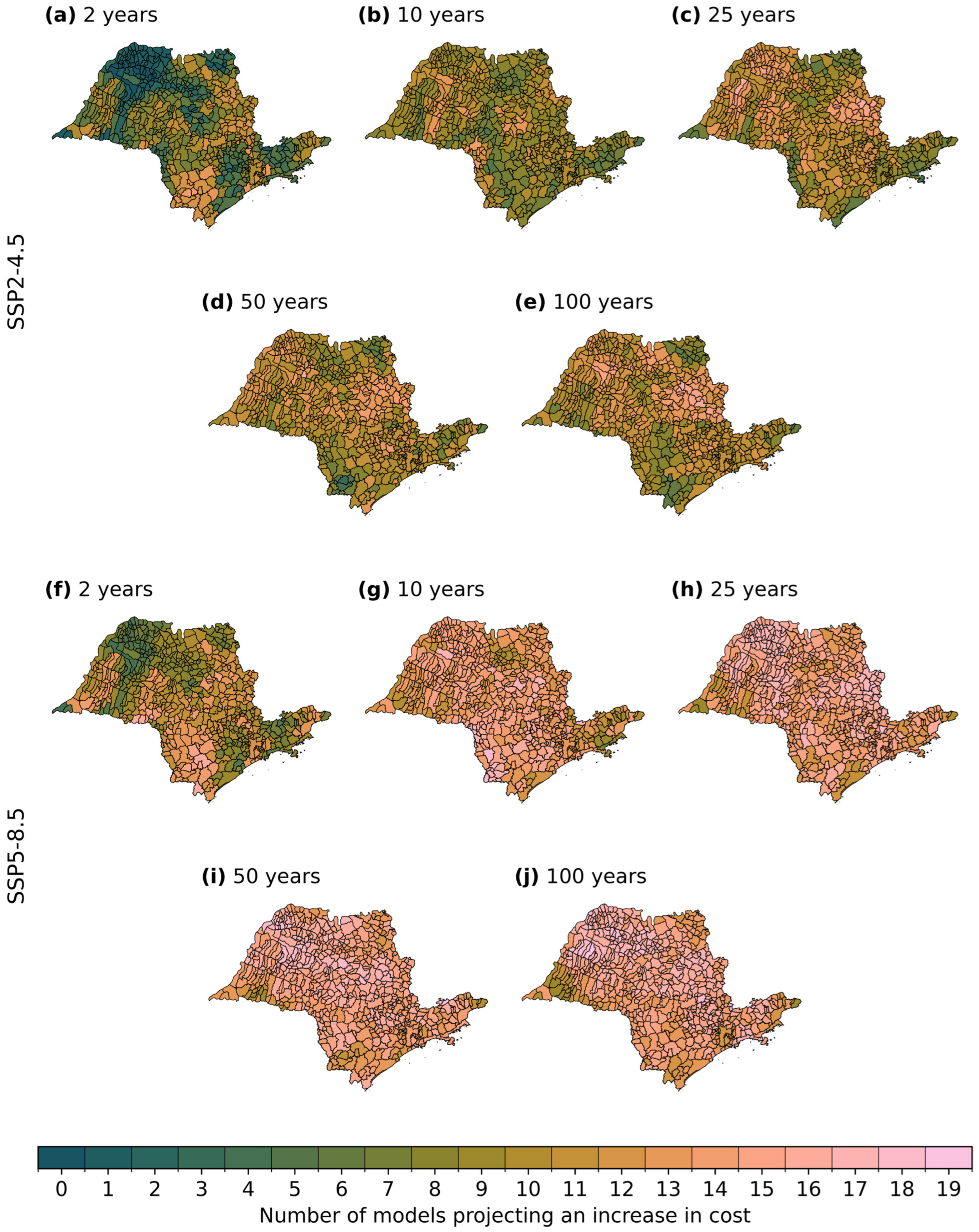
Inter-model sign maps (Figures S10 and S14) show that projected cost decreases are essentially absent: across RPs and both time horizons, only 0–1 models indicate decreases, so negative changes are not an expected outcome. In contrast, neutral outcomes (Figures S11 and S15) are common in the immediate future but decline with increasing RP. Agreement on cost increases (Figure 9 and Figure 10) strengthens markedly from the immediate to the distant future. In the immediate future, at least ten models support increases of 10–53% in municipalities under SSP2-4.5 and 11–48% under SSP5-8.5. In the distant future, agreement becomes widespread, with ≥10-model agreement rising to 30–80% (SSP2-4.5) and 55–99% (SSP5-8.5), increasing with RP. This pattern is consistent with the broader literature showing that, as radiative forcing increases and internal variability becomes less dominant, climate models tend to converge more strongly in the direction of change in extremes. From an engineering perspective, such high levels of agreement strengthen the case for explicitly incorporating non-stationarity into culvert design, particularly for assets with long service lives that will operate well into the distant future.

Although this study focuses explicitly on the rainfall-driven component of nonstationarity, the literature shows that when climate change and urban development are considered simultaneously, existing drainage networks often struggle to cope with the combined pressures, revealing structural and capacity limitations (Kourtis and Tsihrintzis [9], and references therein). These results raise an important design and policy question: while a large portion of the state would, face higher capital expenditures to update design standards, a risk perspective treats these additional expenditures as investments that reduce the probability of structural failure and associated damages under a nonstationary climate. Studies that jointly consider construction and damage costs have shown that proactive adaptation of drainage and related infrastructure can yield substantial avoided damages over the asset lifetime (e.g., [10,11,12]).

3.5. Limitations and Generalization

The analysis focuses on climate-driven nonstationarity while assuming fixed catchment and drainage-system conditions. However, in practice, local land-use and land-cover change, drainage connectivity, and water-management practices also influence infrastructure performance. These factors may interact synergistically with climate change, either amplifying or attenuating pressure on drainage systems. Explicitly accounting for such interactions would require detailed, city-specific data that are not consistently available at the regional scale adopted in this study. In addition, we do not include inlet control and head losses, so absolute dimensions and costs represent first-order, lower bound estimates. Accounting for entrance/exit losses and upstream headwater conditions would generally increase required sizes and costs, although relative spatial patterns and differences between scenarios should be more robust than absolute values.

The study adopts a first-order, exploratory framework that links nonstationary rainfall projections to hydraulic design implications, which helps identify regional patterns and order-of-magnitude effects but does not replace catchment- or project-scale hydrologic–hydraulic modeling. We simplify runoff generation, antecedent soil moisture, and drainage-network configuration, which may affect absolute capacity estimates; results should therefore be interpreted as indicative rather than prescriptive for site-specific design. We disaggregate daily design rainfall to sub-daily durations using municipality-specific reduction factors derived from observation-based gridded IDF information; this captures present-day spatial variability but assumes a stationary within-rainfall temporal structure, so future changes in sub-daily rainfall patterns cannot be directly resolved with daily climate forcing. Although some inputs are Brazil-specific (e.g., disaggregation guidance, hydraulic checks, and official cost databases), the workflow remains transferable, since other regions can apply the same impact chain using local IDF and disaggregation information, rainfall–runoff methods, hydraulic design standards, and unit-cost references.

4. Conclusions

This study demonstrates that flood risk in São Paulo State has intensified over recent decades and is likely to continue increasing under a nonstationary climate. The sharp rise in the number of flood-related events registered, their spatial expansion, and the growing human and economic impacts indicate that risk intensification cannot be attributed to climatic changes alone. Rather, it emerges from the interaction between climatic forcing, catchment state, and structure, and factors related to exposure, vulnerability, and infrastructure limitations, particularly in urbanized and hydrologically modified areas.

By propagating projected changes in extreme rainfall through an event-based design chain, the study quantifies how non-stationarity translates into coupled changes in design discharge ($\mathsf{\Delta }\mathrm{Q}$), effective culvert section ($\mathsf{\Delta }\mathrm{A}$), and construction costs across municipalities. Projections indicate widespread increases in $\mathsf{\Delta }\mathrm{Q}$, with near-term relative changes in the 9–43% range depending on runoff conditions, and stronger upward shifts under SSP5-8.5 toward the late century. When hydraulic requirements are mapped to commercially available nominal sizes, ΔA becomes discretized and exhibits threshold behavior: many municipalities show no nominal change in the immediate future, particularly for small basins and short RPs, while larger catchments cross catalogue thresholds much more frequently. In the distant future, nominal-section upgrades become nearly ubiquitous for A ≥ 125 km², and upper-tail section increases can approach 200% (versus 100% in the immediate future), underscoring the stepwise nature of adaptation needs.

Cost results mirror this catalogue-threshold mechanism. In the immediate future (2015–2055), many municipalities remain close to the baseline, with roughly 68% showing increases of up to 10% for RP ≤ 25 years, while under SSP5-8.5 and for RP > 25 years, approximately 46% of municipalities exceed 10% additional costs, reflecting more frequent and larger nominal-section upgrades for rarer events. By the distant future (2056–2100), the distribution shifts upward and model agreement on cost increases strengthens markedly: decreases become essentially absent, and under SSP5-8.5 about 86% of municipalities exceed 10% cost increases even for RP ≤ 25 years.

From an engineering and planning perspective, these results highlight the limitations of stationary design assumptions for drainage infrastructure with long service lives. The projected increases in culvert size and construction costs should not be interpreted solely as additional financial burdens, but as investments that reduce the likelihood of structural failure and the magnitude of flood damage under future climatic conditions. The magnitude of the projected changes is consistent with uplift factors already adopted in several international guidelines, reinforcing the need for similar, context-specific guidance in Brazil. Overall, this study supports the explicit incorporation of nonstationarity into drainage design and adaptation planning in São Paulo State. Although uncertainties remain regarding future emission trajectories and local-scale responses, the consistent direction and magnitude of the projected changes suggest that delaying adaptation would likely increase long-term costs and risks.

References

1. Ballarin, A.S.; Anache, J.A.; Wendland, E. Trends and abrupt changes in extreme rainfall events and their influence on design quantiles: A case study in São Paulo, Brazil. Theor. Appl. Climatol. 2022, 149, 1753–1767. [Google Scholar] [CrossRef]
2. Milly, P.C.; Betancourt, J.; Falkenmark, M.; Hirsch, R.M.; Kundzewicz, Z.W.; Lettenmaier, D.P.; Stouffer, R.J. Stationarity is dead: Whither water management? Science 2008, 319, 573–574. [Google Scholar] [CrossRef]
3. Perkins-Kirkpatrick, S.; Barriopedro, D.; Jha, R.; Wang, L.; Mondal, A.; Libonati, R.; Kornhuber, K. Extreme terrestrial heat in 2023. Nat. Rev. Earth Environ. 2024, 5, 244–246. [Google Scholar] [CrossRef]
4. Alvalá, R.C.d.S.; Ribeiro, D.F.; Marengo, J.A.; Seluchi, M.E.; Gonçalves, D.A.; da Silva, L.A.; Pineda, L.A.C.; Saito, S.M. Analysis of the hydrological disaster occurred in the state of Rio Grande do Sul, Brazil in September 2023: Vulnerabilities and risk management capabilities. Int. J. Disaster Risk Reduct. 2024, 110, 104645. [Google Scholar] [CrossRef]
5. Brandão, A.R.A.; Schwamback, D.; de Menezes Filho, F.C.; Oliveira, P.T.; Fava, M.C. Artificial Neural Networks for Flood Prediction in Current and CMIP6 Climate Change Scenarios. J. Flood Risk Manag. 2025, 18, e70029. [Google Scholar] [CrossRef]
6. Ballarin, A.S.; Vargas Godoy, M.R.; Zaerpour, M.; Abdelmoaty, H.M.; Hatami, S.; Gavasso-Rita, Y.L.; Wendland, E.; Papalexiou, S.M. Drought intensification in Brazilian catchments: Implications for water and land management. Environ. Res. Lett. 2024, 19, 054030. [Google Scholar] [CrossRef]
7. de Lima, L.S.; Silva, F.E.O.; Anastácio, P.R.D.; Kolanski, M.M.d.P.; Pereira, A.C.P.; Menezes, M.S.R.; Cunha, E.L.T.P.; Macedo, M.N. Severe droughts reduce river navigability and isolate communities in the Brazilian Amazon. Commun. Earth Environ. 2024, 5, 370. [Google Scholar] [CrossRef]
8. Schwamback, D.; Brandão, A.R.A.; Berndtsson, R.; Wendland, E.; Persson, M. Assessment of water fluxes under the dual threat of changes in land cover and climate variability in the Brazilian Cerrado biome. J. Hydrol. Reg. Stud. 2025, 61, 102699. [Google Scholar] [CrossRef]
9. Kourtis, I.M.; Tsihrintzis, V.A. Adaptation of urban drainage networks to climate change: A review. Sci. Total Environ. 2021, 771, 145431. [Google Scholar] [CrossRef]
10. Neumann, J.E.; Price, J.; Chinowsky, P.; Wright, L.; Ludwig, L.; Streeter, R.; Jones, R.; Smith, J.B.; Perkins, W.; Jantarasami, L.; et al. Climate change risks to US infrastructure: Impacts on roads, bridges, coastal development, and urban drainage. Clim. Change 2015, 131, 97–109. [Google Scholar] [CrossRef]
11. Martel, J.L.; Brissette, F.P.; Lucas-Picher, P.; Troin, M.; Arsenault, R. Climate change and rainfall intensity–duration–frequency curves: Overview of science and guidelines for adaptation. J. Hydrol. Eng. 2021, 26, 03121001. [Google Scholar] [CrossRef]
12. Dottori, F.; Mentaschi, L.; Bianchi, A.; Alfieri, L.; Feyen, L. Cost-effective adaptation strategies to rising river flood risk in Europe. Nat. Clim. Change 2023, 13, 196–202. [Google Scholar] [CrossRef]
13. Cheng, L.; AghaKouchak, A. Nonstationary precipitation intensity-duration-frequency curves for infrastructure design in a changing climate. Sci. Rep. 2014, 4, 7093. [Google Scholar] [CrossRef]
14. Arheimer, B.; Cudennec, C.; Castellarin, A.; Grimaldi, S.; Heal, K.V.; Lupton, C.; Sarkar, A.; Tian, F.; Onema, J.-M.K.; Archfield, S.; et al. The IAHS science for solutions decade, with hydrology engaging local people in one global world (HELPING). Hydrol. Sci. J. 2024, 69, 1417–1435. [Google Scholar] [CrossRef]
15. Madsen, H.; Lawrence, D.; Lang, M.; Martinkova, M.; Kjeldsen, T.R. Review of trend analysis and climate change projections of extreme precipitation and floods in Europe. J. Hydrol. 2014, 519, 3634–3650. [Google Scholar] [CrossRef]
16. Paiva, R.; Collischonn, W.; Miranda, P.; Petry, I.; Dornelles, F.; Goldenfum, J.; Fan, F.; Ruhoff, A.; Fagundes, H. Critérios hidrológicos para adaptação à mudança climática: Chuvas e cheias extremas na Região Sul do Brasil (Nota Técnica); Instituto de Pesquisas Hidráulicas, Universidade Federal do Rio Grande do Sul (IPH/UFRGS): Porto Alegre, Brazil, 2024; Available online: https://www.ufrgs.br/iph/wp-content/uploads/2024/05/CriteriosAdaptacaoMudancaClimaticaChuvasCheiasExtremasSul.pdf (accessed on 10 November 2025).
17. Defra. Guidance—Flood and Coastal Risk Projects, Schemes and Strategies: Climate Change Allowance. Available online: https://www.gov.uk/guidance/flood-and-coastal-risk-projects-schemes-and-strategies-climate-change-allowances (accessed on 12 December 2025).
18. Cannon, A.J.; Jeong, D.I.; Zhang, X.; Zwiers, F.W. Climate-Resilient Buildings and Core Public Infrastructure: An Assessment of the Impact of Climate Change on Climatic Design Data in Canada; Government of Canada: Ottawa, ON, Canada, 2020; 106p. [Google Scholar]
19. Adam, D. What a 190-year-old equation says about rainstorms in a changing climate. Proc. Natl. Acad. Sci. USA 2023, 120, e2304077120. [Google Scholar] [CrossRef]
20. Andria, S.; Borga, M.; Marani, M. Thermodynamic versus large-scale controls on extreme precipitation: Temporal scale dependence and Clausius-Clapeyron scaling redefined. Geophys. Res. Lett. 2025, 52, e2025GL115204. [Google Scholar] [CrossRef]
21. Silva, N.A.; Haerter, J.O. Super-Clausius–Clapeyron scaling of extreme precipitation explained by shift from stratiform to convective rain type. Nat. Geosci. 2025, 18, 382–388. [Google Scholar] [CrossRef]
22. Ball, J.; Babister, M.; Nathan, R.; Weeks, W.; Weinmann, E.; Retallick, M.; Testoni, I. (Eds.) Australian Rainfall and Runoff: A Guide to Flood Estimation (Version 4.2); Commonwealth of Australia (Geoscience Australia): Barton, ACT, Australia, 2019; ISBN 978-1-925848-36-6. [Google Scholar]
23. Wasko, C.; Westra, S.; Nathan, R.; Pepler, A.; Raupach, T.H.; Dowdy, A.; Johnson, F.; Ho, M.; McInnes, K.L.; Jakob, D.; et al. A systematic review of climate change science relevant to Australian design flood estimation. Hydrol. Earth Syst. Sci. 2024, 28, 1251–2024. [Google Scholar] [CrossRef]
24. Saboia, M.A.M.; de Souza Filho, F.D.A.; Helfer, F.; Rolim, L.Z.R. Robust strategy for assessing the costs of urban drainage system designs under climate change scenarios. J. Water Resour. Plan. Manag. 2020, 146, 05020022. [Google Scholar] [CrossRef]
25. Kourtis, I.M.; Tsihrintzis, V.A. Update of intensity-duration-frequency (IDF) curves under climate change: A review. Water Supply 2022, 22, 4951–4974. [Google Scholar] [CrossRef]
26. Silva, D.F.; Goldenfum, J.A.; Simonovic, S.P.; Dornelles, F. Impacts of climate change on the intensity-duration-frequency curves of two urbanized areas in Brazil using the high-resolution Eta atmospheric model. Urban Water J. 2023, 20, 123–139. [Google Scholar] [CrossRef]
27. Schlef, K.E.; Kunkel, K.E.; Brown, C.; Demissie, Y.; Lettenmaier, D.P.; Wagner, A.; Wigmosta, M.S.; Karl, T.R.; Easterling, D.R.; Wang, K.J.; et al. Incorporating non-stationarity from climate change into rainfall frequency and intensity-duration-frequency (IDF) curves. J. Hydrol. 2023, 616, 128757. [Google Scholar] [CrossRef]
28. Abdelmoaty, H.M.; Papalexiou, S.M. Changes of extreme precipitation in CMIP6 projections: Should we use stationary or nonstationary models? J. Clim. 2023, 36, 2999–3014. [Google Scholar] [CrossRef]
29. Doulabian, S.; Tousi, E.G.; Shadmehri Toosi, A.; Alaghmand, S. Non-stationary precipitation frequency estimates for resilient infrastructure design in a changing climate: A case study in Sydney. Hydrology 2023, 10, 117. [Google Scholar] [CrossRef]
30. Gründemann, G.J.; van de Giesen, N.; Brunner, L.; van der Ent, R. Rarest rainfall events will see the greatest relative increase in magnitude under future climate change. Commun. Earth Environ. 2022, 3, 235. [Google Scholar] [CrossRef]
31. Ballarin, A.S.; Wendland, E.; Zaerpour, M.; Hatami, S.; Meira Neto, A.A.; Papalexiou, S.M. Frequency rather than intensity drives projected changes of rainfall events in Brazil. Earth’s Future 2024, 12, e2023EF004053. [Google Scholar] [CrossRef]
32. Sharma, A.; Wasko, C.; Lettenmaier, D.P. If precipitation extremes are increasing, why aren’t floods? Water Resour. Res. 2018, 54, 8545–8551. [Google Scholar] [CrossRef]
33. Wasko, C.; Sharma, A.; Lettenmaier, D.P. Increases in temperature do not translate to increased flooding. Nat. Commun. 2019, 10, 5676. [Google Scholar] [CrossRef]
34. Obara, C.; Fletcher, C.H.; Habel, S.; McDonald, K.; Yamamoto, K. Drainage failure and associated urban impacts under combined sea-level rise and precipitation scenarios. Sci. Rep. 2025, 15, 23436. [Google Scholar] [CrossRef]
35. World Meteorological Organization (WMO). WMO Atlas of Mortality and Economic Losses from Weather, Climate and Water Extremes (1970–2019); WMO-No. 1267; World Meteorological Organization: Geneva, Switzerland, 2021; ISBN 978-92-63-11267-5. [Google Scholar]
36. Mendes, A.T.; dos Santos, G.R.; de Albuquerque Alves, C. Trajectory, challenges, and opportunities in Sustainable Urban Water Management in Brazil: Nature-based solutions for urban stormwater drainage. In Nature-Based Solutions for Circular Management of Urban Water; Springer Nature: Berlin/Heidelberg, Germany, 2024; pp. 295–313. [Google Scholar] [CrossRef]
37. Haddad, E.A.; Teixeira, E. Economic impacts of natural disasters in megacities: The case of floods in São Paulo, Brazil. Habitat Int. 2015, 45, 106–113. [Google Scholar] [CrossRef]
38. Chambwera, M.; Heal, G.; Dubeux, C.; Hallegatte, S.; Leclerc, L.; Markandya, A.; McCarl, B.A.; Mechler, R.; Neumann, J.E. Chapter 17—Economics of adaptation. In Climate Change 2014: Impacts, Adaptation, and Vulnerability. Part A: Global and Sectoral Aspects. Contribution of Working Group II to the Fifth Assessment Report of the IPCC; Cambridge University Press: Cambridge, UK; New York, NY, USA, 2014. [Google Scholar]
39. Wasko, C.; Nathan, R.; Stein, L.; O’Shea, D. Evidence of shorter more extreme rainfalls and increased flood variability under climate change. J. Hydrol. 2021, 603, 126994. [Google Scholar] [CrossRef]
40. Instituto Brasileiro de Geografia e Estatística (IBGE). Censo Demográfico. Available online: https://www.ibge.gov.br/estatisticas/sociais/populacao/22827-censo-demografico-2022.html?edicao=381 (accessed on 1 November 2025).
41. Alvares, C.A.; Stape, J.L.; Sentelhas, P.C.; Gonçalves, J.D.M.; Sparovek, G. Köppen’s climate classification map for Brazil. Meteorol. Z. 2013, 22, 711–728. [Google Scholar] [CrossRef]
42. Funk, C.; Peterson, P.; Landsfeld, M.; Pedreros, D.; Verdin, J.; Shukla, S.; Husak, G.; Rowland, J.; Harrison, L.; Hoell, A.; et al. The Climate Hazards Infrared Precipitation with Stations—A New Environmental Record for Monitoring Extremes. Sci. Data 2015, 2, 150066. [Google Scholar] [CrossRef]
43. São Paulo (State), Secretariat for the Environment; Environmental Planning Coordination. Modelo Digital de Elevação (MDE) do Estado de São Paulo obtido a partir da base do Projeto GISAT (cartas topográficas na escala 1:50.000) [Technical Documentation]. 2013. Available online: https://smastr16.blob.core.windows.net/cpla/2013/10/Ficha_Tecnica_MDE.pdf (accessed on 1 November 2025).
44. Brazil, Ministry of Regional Development; National Secretariat for Protection and Civil Defense. Digital Atlas of Disasters in Brazil, 2025. Available online: https://atlasdigital.mdr.gov.br/paginas/mapa-interativo.xhtml (accessed on 5 November 2025).
45. Ballarin, A.S.; Sone, J.S.; Gesualdo, G.C.; Schwamback, D.; Reis, A.; Almagro, A.; Wendland, E.C. CLIMBra-climate change dataset for Brazil. Sci. Data 2023, 10, 47. [Google Scholar] [CrossRef]
46. Cannon, A.J.; Sobie, S.R.; Murdock, T.Q. Bias correction of GCM precipitation by quantile mapping: How well do methods preserve changes in quantiles and extremes? J. Clim. 2015, 28, 6938–6959. [Google Scholar] [CrossRef]
47. Beck, H.E.; Wood, E.F.; Pan, M.; Fisher, C.K.; Miralles, D.G.; van Dijk, A.I.J.M.; McVicar, T.R.; Adler, R.F. MSWEP V2 global 3-hourly 0.1 precipitation: Methodology and quantitative assessment. Bull. Am. Meteorol. Soc. 2019, 100, 473–500. [Google Scholar] [CrossRef]
48. Xavier, A.C.; King, C.W.; Scanlon, B.R. Daily gridded meteorological variables in Brazil (1980–2013). Int. J. Climatol. 2016, 36, 2644–2659. [Google Scholar] [CrossRef]
49. Ballarin, A.S.; Calixto, K.G.; Anache, J.A.; Wendland, E. Combined predictive and descriptive tests for extreme rainfall probability distribution selection. Hydrol. Sci. J. 2022, 67, 1130–1140. [Google Scholar] [CrossRef]
50. Montanari, A.; Koutsoyiannis, D. Modeling and mitigating natural hazards: Stationarity is immortal! Water Resour. Res. 2014, 50, 9748–9756. [Google Scholar] [CrossRef]
51. Koutsoyiannis, D.; Montanari, A. Negligent killing og scientific concepts: The stationarity case. Hydrol. Sci. J. 2015, 60, 1174–1183. [Google Scholar] [CrossRef]
52. Lins, H.F.; Cohn, T.A. Stationarity: Wanted dead or alive? J. Am. Water Resour. Assoc. 2011, 47, 475–480. [Google Scholar] [CrossRef]
53. Cook, L.M.; McGinnis, S.; Samaras, C. The effect of modeling choices on updating intensity-duration-frequency curves and stormwater infrastructure designs for climate change. Clim. Change 2020, 159, 289–308. [Google Scholar] [CrossRef]
54. Sharma, S.; Lee, B.S.; Nicholas, R.E.; Keller, K. A safety factor approach to designing urban infrastructure for dynamic conditions. Earth’s Future 2021, 9, e2021EF002118. [Google Scholar] [CrossRef]
55. Ponce, V.M.; Hawkins, R.H. Runoff curve number: Has it reached maturity? J. Hydrol. Eng. 1996, 1, 11–19. [Google Scholar] [CrossRef]
56. CETESB. Drenagem Urbana: Manual de Projeto; CETESB: São Paulo, Brazil, 1986. Available online: https://repositorio.cetesb.sp.gov.br/handle/123456789/2863 (accessed on 5 November 2025).
57. Hawkins, R.H.; Ward, T.J.; Woodward, D.E.; Van Mullem, J.A. (Eds.) Curve Number Hydrology: State of the Practice; American Society of Civil Engineers: Reston, VA, USA, 2009. [Google Scholar]
58. Brandão, A.R.A.; Schwamback, D.; Ballarin, A.S.; Ramirez-Avila, J.J.; Neto, J.G.V.; Oliveira, P.T.S. Toward a better understanding of curve number and initial abstraction ratio values from a large sample of watersheds perspective. J. Hydrol. 2025, 655, 132941. [Google Scholar] [CrossRef]
59. Galbetti, M.V.; Zuffo, A.C.; Shinma, T.A.; Boulomytis, V.T.G.; Imteaz, M. Evaluation of the tabulated, NEH4, least squares and asymptotic fitting methods for the CN estimation of urban watersheds. Urban Water J. 2022, 19, 244–255. [Google Scholar] [CrossRef]
60. Simpson, I.M.; Winston, R.J.; Tirpak, R.A.; Dorsey, J.D.; Stagge, J.H.; Hathaway, J.M. Hydrologic responses of single land use urban and forested watersheds and their implications to improving urban drainage design. J. Hydrol. 2023, 620, 129430. [Google Scholar] [CrossRef]
61. Bonta, J.; Chin, D.A.; Johnson, M.S.; Miller, J.J.; Minervini, W.; Ramirez-Avila, J.; Moglen, G.; Neelam, T.J.; Oliveira, P.T.S.; Sharma, S.; et al. The Curve Number’s Initial Abstraction and Physical Hydrology: ASCE-EWRI CN Hydrology Committee Synthesis. J. Irrig. Drain. Eng. 2025, 151, 06025002. [Google Scholar] [CrossRef]
62. USDA-NRCS. National Engineering Handbook, Title 210, Part 630–Hydrology, Subpart H: Estimation of Direct Runoff from Storm Rainfall; U.S. Department of Agriculture, Natural Resources Conservation Service (eDirectives): Washington, DC, USA, 2025.
63. Chin, D.A. Estimating peak runoff rates using the rational method. J. Irrig. Drain. Eng. 2019, 145, 04019006. [Google Scholar] [CrossRef]
64. Gomes, M.N., Jr. Gridded Bias-Corrected Intensity-Duration-Frequency Curves for Brazil Using BR-DWGD, IMERG, CHRIPS, and PERSIANN Datasets with Locally-Derived Disaggregation Coefficients. Available online: https://ssrn.com/abstract=5589326 (accessed on 1 February 2026). [CrossRef]
65. DNIT (Departamento Nacional de Infraestrutura de Transportes). Manual de Drenagem de Rodovias, 2nd ed.; IPR Publ. 724; Instituto de Pesquisas Rodoviárias, DNIT: Rio de Janeiro, Brazil, 2006. Available online: https://www.gov.br/dnit/pt-br/assuntos/planejamento-e-pesquisa/ipr/coletanea-de-manuais/vigentes/724_manual_drenagem_rodovias.pdf (accessed on 20 November 2025).
66. Baptista, M.B.; Coelho, M.M.L.P. Fundamentos de Engenharia Hidráulica, 4th ed.; Editora UFMG: Belo Horizonte, Brazil, 2016. [Google Scholar]
67. SINAPI. National System of Construction Costs and Indexes. Caixa Econômica Federal. 2025. Available online: https://www.caixa.gov.br/sinapi (accessed on 20 October 2025).
68. SICRO. SICRO–Federal Highway Works Cost System. National Department of Transport Infrastructure (DNIT). 2025. Available online: https://www.gov.br/dnit (accessed on 20 October 2025).
69. SIURB. SIURB–Urban Infrastructure Cost System. São Paulo Municipal Secretariat of Urban Infrastructure and Works, 3 November 2025. Available online: https://www.prefeitura.sp.gov.br (accessed on 20 October 2025).
70. TCU. Ruling No. 2622/2013. Federal Court of Audit (Tribunal de Contas da União). 2013. Available online: https://www.tcu.gov.br (accessed on 20 October 2025).
71. Marengo, J.A.; Ambrizzi, T.; Alves, L.M.; Barreto, N.J.; Simões Reboita, M.; Ramos, A.M. Changing trends in rainfall extremes in the metropolitan area of São Paulo: Causes and impacts. Front. Clim. 2020, 2, 3. [Google Scholar] [CrossRef]
72. Silva, R.C.; Marengo, J.A.; Ruv Lemes, M. Analysis of extreme rainfall and landslides in the metropolitan region of the Paraiba do Sul River Valley and North Coast of Sao Paulo, Brazil. Theor. Appl. Climatol. 2024, 155, 3927–3949. [Google Scholar] [CrossRef]
73. Kang, M.S.; Koo, J.H.; Chun, J.A.; Her, Y.G.; Park, S.W.; Yoo, K. Design of drainage culverts considering critical storm duration. Biosyst. Eng. 2009, 104, 425–434. [Google Scholar] [CrossRef]
74. Ragno, E.; AghaKouchak, A.; Love, C.A.; Cheng, L.; Vahedifard, F.; Lima, C.H. Quantifying changes in future intensity-duration-frequency curves using multimodel ensemble simulations. Water Resour. Res. 2018, 54, 1751–1764. [Google Scholar] [CrossRef]
75. Niemczynowicz, J. Impact of the greenhouse effect on sewerage systems—Lund case study. Hydrol. Sci. J. 1989, 34, 651–666. [Google Scholar] [CrossRef]
76. Arnbjerg-Nielsen, K. Quantification of climate change effects on extreme precipitation used for high resolution hydrologic design. Urban Water J. 2012, 9, 57–65. [Google Scholar] [CrossRef]
77. Welsh Government. Climate Change Allowances and Flood Consequence Assessments. 2021. Available online: https://www.gov.wales/climate-change-allowances-and-flood-consequence-assessments (accessed on 1 September 2025).
78. ANA. Impacts of Climate Change on Water Resources in Brazil: Executive Summary; National Water and Basic Sanitation Agency (Agência Nacional de Águas e Saneamento Básico): Brasília, Brazil, 2024. Available online: https://www.gov.br/ana (accessed on 17 December 2025).
79. Pillar, V.D.; Overbeck, G.E. Learning from a climate disaster: The catastrophic floods in southern Brazil. Science 2024, 385, eadr8356. [Google Scholar] [CrossRef]
80. Hausfather, Z.; Peters, G.P. Emissions–the ‘business as usual’ story is misleading. Nature 2020, 577, 618–620. [Google Scholar] [CrossRef] [PubMed]
81. Sanford, T.; Frumhoff, P.C.; Luers, A.; Gulledge, J. The climate policy narrative for a dangerously warming world. Nat. Clim. Change 2014, 4, 164–166. [Google Scholar] [CrossRef]
82. Schwalm, C.R.; Glendon, S.; Duffy, P.B. RCP8.5 tracks cumulative CO2 emissions. Proc. Natl. Acad. Sci. USA 2020, 117, 19656–19657. [Google Scholar] [CrossRef]
Figure 1. Location of the study area. (a) Spatial distribution of mean daily rainfall (mm.day−1) over São Paulo State for 1981–2013 derived from CHIRPS v2.0 [42] and (b) Topography from the São Paulo State (30 m horizontal resolution; SIRGAS 2000) obtained from [43].
Water 18 00561 g001
Figure 2. Flood-related events in the São Paulo State, Brazil (1991–2024). (a) Total number of recorded flood events per decade. (b) Number of municipalities reporting at least one flood-related event (≥1 event) per decade. (c) Spatial distribution of the cumulative number of flood events at the municipal scale (counts).
Water 18 00561 g002
Figure 3. Projected change in design discharge (ΔQ) versus return period (RP) for Tc = D = 1, 6, and 24 h and curve numbers (CN) of 50, 75, and 98 in the immediate future (2015–2055) relative to the baseline (1980–2013). Panels (ac) show Tc = D = 1 h, (df) Tc = D = 6 h, and (gi) Tc = D = 24 h. In each row, CN increases from left to right (50, 75, 98). Curves are shown for catchment areas A = 3, 125, and 250 km2 under SSP2-4.5 and SSP5-8.5. Lines show the across-municipality median ΔQ, and shaded bands show the 10th–90th percentile range (based on per-municipality medians across climate models).
Water 18 00561 g003
Figure 4. Projected change in design discharge (ΔQ) versus return period (RP) for Tc = D = 1, 6, and 24 h and curve numbers (CN) of 50, 75, and 98 in the distant future (2056–2100) relative to the baseline (1980–2013). Panels (ac) show Tc = D = 1 h, (df) Tc = D = 6 h, and (gi) Tc = D = 24 h. In each row, CN increases from left to right (50, 75, 98). Curves are shown for catchment areas A = 3, 125, and 250 km2 under SSP2-4.5 and SSP5-8.5. Lines show the across-municipality median ΔQ, and shaded bands show the 10th–90th percentile range (based on per-municipality medians across climate models).
Water 18 00561 g004
Figure 5. Empirical cumulative distribution functions (ECDFs) of projected relative changes in required culvert area (ΔA) across municipalities in the immediate future (2015–2055) relative to the baseline (1980–2013). Panels (ao) correspond to return periods of 2, 10, 25, 50, and 100 years, while columns correspond to curve numbers CN = 50, 75, and 98. Curves represent catchment areas A = 3, 125, and 250 km2 under SSP2-4.5 and SSP5-8.5.
Water 18 00561 g005
Figure 6. Empirical cumulative distribution functions (ECDFs) of projected relative changes in required culvert area (ΔA) across municipalities in the distant future (2056–2100) relative to the baseline (1980–2013). Panels (ao) correspond to return periods of 2, 10, 25, 50, and 100 years, while columns correspond to curve numbers CN = 50, 75, and 98. Curves represent catchment areas A = 3, 125, and 250 km2 under SSP2-4.5 and SSP5-8.5.
Water 18 00561 g006
Figure 7. Relative changes in culvert construction costs across municipalities in São Paulo State for the immediate-future period (2015–2055), referenced to the baseline period (1980–2013, shown as the ensemble mean and for different RP. Panels are organized by scenario, with SSP2-4.5 in the top two rows and SSP5-8.5 in the bottom two rows, and panels (aj) show results for different RP.
Water 18 00561 g007
Figure 8. Relative changes in culvert construction costs across municipalities in São Paulo State for the distant-future period (2056–2100), referenced to the baseline period (1980–2013), shown as the ensemble mean and for different RP. Panels are organized by scenario, with SSP2-4.5 in the top two rows and SSP5-8.5 in the bottom two rows, and panels (aj) show results for different RP.
Water 18 00561 g008
Figure 9. Number of climate models projecting an increase in culvert construction costs across municipalities in São Paulo State for the immediate-future period (2015–2055), relative to the baseline period (1980–2013). Panels are organized by scenario, with SSP2-4.5 in the top two rows and SSP5-8.5 in the bottom two rows, and panels (aj) show results for different RP.
Water 18 00561 g009
Figure 10. Number of climate models projecting an increase in culvert construction costs across municipalities in São Paulo State for the distant-future period (2056–2100), relative to the baseline period (1980–2013). Panels are organized by scenario, with SSP2-4.5 in the top two rows and SSP5-8.5 in the bottom two rows, and panels (aj) show results for different RP.
Water 18 00561 g010
Disclaimer/Publisher’s Note: The statements, opinions and data contained in all publications are solely those of the individual author(s) and contributor(s) and not of MDPI and/or the editor(s). MDPI and/or the editor(s) disclaim responsibility for any injury to people or property resulting from any ideas, methods, instructions or products referred to in the content.