


Abstract
Water-quality degradation from nutrient pollution remains a major challenge for resource managers. Developing effective strategies requires tools to characterize nutrient sources and transport. This study used the RSPARROW framework to develop and assess new, smaller-scale models for Total Nitrogen (TN) and Total Phosphorus (TP) transport across Mississippi (MS). These state-level models were built using 15 years (2005–2020) of observation data and considered variables including multiple nutrient sources, land characteristics, and attenuation processes. The MS models demonstrated comparable accuracy to larger regional SPARROW models, validating the use of smaller-scale models for local management. Results showed agricultural sources are the major contributors to TN, dominated by fertilizer in northern MS and livestock manure in the south. Urban land cover also significantly influenced TN and was the second most significant source of TP, following geologic material (background P). Fertilizer and manure were also important TP sources. This study provides valuable, spatially explicit data on nutrient distribution in MS streams, supporting the state’s nutrient reduction planning. It concludes by highlighting the need for future model improvements via updated source data and mean annual flow estimates.
1. Introduction
The pollution of aquatic environments from nutrients leads to a process known as eutrophication. During eutrophication, excessive nutrients cause proliferation of aquatic vegetation and microorganisms, resulting in the depletion of dissolved oxygen and degradation of aquatic environments. Many studies have shown the effects of eutrophication on aquatic environments ranging from changes in the assemblages of aquatic vegetation [1,2,3], food web dynamics in aquatic and marine ecosystems [4,5,6], increasing primary productivity [7,8,9], decreasing biodiversity [10], and increasing turbidity [11]. Moreover, eutrophication affects fish communities [12,13,14], wildlife [15,16], and livestock [17]. Eutrophication is also a threat to human health by encouraging the proliferation of cyanobacteria that produce toxic metabolites [18].
In littoral zones (e.g., near-shore, lakes), eutrophication occurs when excess nutrients stimulate an overgrowth of algae, characterized by excess growth of dense mats of algae that block sunlight from reaching aquatic vegetation, and the subsequent microbial decomposition of the algae and plant detritus consumes oxygen, producing hypoxic zones [19]. Stimulated by excess nutrients from the Mississippi/Atchafalaya River Basin, one of the most extensive hypoxic zones occurs in the Gulf of America over the Louisiana-Texas shelf [20].
Anthropogenic sources of nutrients include wastewater effluent, runoff from agriculture and pasture, and urban runoff. Fossil fuel combustion also contributes nitrogen (N) to watersheds through atmospheric deposition, and phosphorus (P) can enter streams through soil erosion [21]. In the Mississippi Alluvial Plain (MAP), a large ecoregion in northwest Mississippi, agriculture accounts for roughly 65% of land use and 25% is classified as wetland [22]. The 2012 Midwest SPARROW (Spatially Referenced Regression On Watershed attributes) model [23] predicts fertilizer as the greatest source of P in this region, while atmospheric deposition, N fixation, and fertilizer are major contributors of N. Manure is a major source of P and N in southern central Mississippi, a region with a high number of broiler chickens [24].
The State of Mississippi has demonstrated a strategic commitment to a localized approach to nutrient management. The Mississippi Department of Environmental Quality (MDEQ) assessed approximately 11% of Mississippi’s 26,370 miles of perennial rivers and streams for the 2022 §305(b) Water-Quality Assessment Report [25]. Fifty four percent of assessed rivers and streams designated for recreational use were deemed impaired, in addition to 57% of the public beaches in MS designated as impaired from non-point source pollution urban runoff [25]. Of waterbodies designated for aquatic life use support, 41% were impaired. Nutrients were cited as a cause for 14% of impairments [25]. In their efforts to reduce excessive nutrient loading, MDEQ has implemented nutrient reduction strategies in the MAP, upland, and coastal regions [26]. MDEQ has developed tailored regional nutrient reduction strategies for the Delta, Upland, and Coastal regions of the state, which have been consolidated into a comprehensive, state-level approach. This management framework is a direct response to the distinct regional differences that exist for nutrient sources across the state. For instance, the MAP strategy focuses on row-crop agriculture, while coastal strategies address issues related to urban runoff and livestock. MDEQ’s nonpoint source pollution program recognizes that urban runoff, from sources such as lawns and roads, is a leading cause of water-quality problems in the state. This issue is managed at the municipal level, as evidenced by MDEQ’s mandate for cities like Biloxi to have a stormwater management plan. A state-level model can provide a more accurate picture of urban nutrient loads, helping to justify the funding and enforcement of stormwater controls. This provides a science-based rationale for addressing a different set of stakeholders and pollutant sources than agriculture and supports a historically under-addressed area of nonpoint source management.
Effective management strategies that aim to reduce nutrient pollution in streams rely upon understanding the sources of nutrients and the factors that influence their delivery to streams. Estimates provided by models of nutrient concentrations and loads in unmonitored streams can be a valuable tool for management, as they can help overcome the challenges of limited data availability and financial constraints. The relative contribution of nutrients from different sources can be estimated with process-based models such as SWAT [27], HYPE [28], and HSPF. However, process-based models require additional post-model analysis to determine the uncertainty of source coefficients, whereas statistical models evaluate coefficient uncertainty directly. SPARROW is a hybrid statistical and process-based mass balance model that predicts the movement of contaminants in streams under long-term, steady state conditions [29]. SPARROW incorporates data on catchment attributes into its predictions, including contaminant sources, landscape characteristics, and streamflow properties, which gives users the ability to identify statistically significant controls on contaminant transport while disregarding factors that are not.
Regional-scale models, such as a typical application of the SPARROW model, are essential scientific tools for characterizing broad environmental processes across large geographic areas. These models are thus well-suited for national or basin-wide assessments and for informing federal policy. The 2012 Midwest SPARROW model [23] and 2012 Southeast SPARROW model [30] encompass the western and eastern halves of Mississippi, respectively. The spatial scales of the 2012 regional models encompass a wide range of landscape characteristics, streamflow conditions, and contaminant sources. As a result, the regional models have substantial statistical power to identify processes affecting the contaminant transport at a level of detail that may be difficult to replicate at small spatial scales or in areas where watershed characteristics are less variable. This feature of large-scale SPARROW models is afforded by the inclusion of hundreds of calibration sites that are necessary to characterize conditions affecting contaminant transport across the entire model domain. During model development, this means the models have a large degree of freedom that enables the inclusion of more explanatory variables in the final models. However, a fundamental limitation of these large-scale models is their inherent averaging effect, which may result in predictions that are biased for a particular subregion [31]. This bias is not a defect, but in some regards an unavoidable consequence of models designed to predict large spatial scales given their tendency towards generalization. These models attempt to synthesizes a vast range of heterogeneous landscapes, land uses, and hydrologic conditions into a single, cohesive framework. Therefore, while regional models may encompass a wide range of agricultural practices, topography, and hydrologic features, many of these features and variability differ from those found in Mississippi. This broad aggregation necessarily smooths out the local variations that are crucial for targeted policymaking at the local level. In this study, we propose a state-level model, which by contrast, can be calibrated to the specific landscape characteristics of Mississippi. The goal of this approach is to provide watershed managers with a tool that is a more accurate representation of Mississippi’s unique environmental context and offer a more customizable and actionable tool for state-level decision-making.
Effective water-quality management, particularly for complex nonpoint source pollution, is ultimately a local endeavor. The scientific literature emphasizes the need for models to function at multiple spatiotemporal scales to capture structure in environmental heterogeneity to be useful for policy [32,33]. For example, the influence of landscape types on water quality can be highly sensitive to spatial and seasonal scales [33,34,35]. A state-level model, which can be developed with a finer-scale resolution and data specific to Mississippi, is best positioned to capture these nuances. The objective is not to replace the valuable regional models but to supplement them with a tool that is fit for a different purpose. This is consistent with a two-layered modeling concept, where a coarse-resolution model can be used for broad applications, while a finer-scale model is available when more detail is needed. For MDEQ, a state-level SPARROW model would be the finer-scale tool, providing the predictive capacity required for applications such as the implementation of state-specific nutrient reduction strategies. The model would be a useful tool for identifying where and how pollution is generated and transported within the state, transforming scientific abstraction into actionable management insight.
The proposed state-level SPARROW model can be used as a scientific counterpart to this administrative and policy structure by providing a data-driven basis for MDEQ’s overarching strategic questions, such as what levels of reduction are achievable and at what cost in different areas across the state. A key function of a state-level model is to act as a strategic scout, identifying high-priority areas where localized management tools will have the greatest impact. A state-level SPARROW model can proactively identify and map watersheds with excess nutrients based on its spatially detailed catchment data. This predictive capacity allows water resource managers to target their outreach and conservation efforts toward areas where these tools are most urgently needed.
The Rotten Bayou watershed project further demonstrates this need for granular modeling capacity. This project, a local-scale implementation of MDEQ’s Coastal Nutrient Reduction Strategy, involved the installation of specific agricultural and urban Best Management Practices (BMPs) by local landowners [36]. A state-level model could provide the necessary pre-project baseline and post-project tracking to rigorously quantify the project’s effectiveness. This quantitative framework is essential for demonstrating the impact of implemented BMPs and for securing future federal funding, such as Clean Water Act Section 319 grants, for similar projects across the state.
The proposed development of state-level SPARROW models for Mississippi is a strategic and necessary undertaking. It represents a critical evolution in the state’s capacity for environmental stewardship, moving beyond the generalized predictions of regional models to provide the granular, spatially explicit data essential for effective, on-the-ground management. The model directly addresses the state’s legal mandates under the Clean Water Act and aligns perfectly with MDEQ’s existing policy framework of developing regionally tailored nutrient reduction strategies. By providing accurate, subregional load and source estimates, the model will empower MDEQ to answer its own critical strategic questions regarding achievable nutrient reductions and their associated costs. Furthermore, the model will serve as a critical tool for securing federal funding, justifying targeted investments, and fostering collaboration among diverse stakeholders by providing a common, scientifically defensible foundation for decision-making. In sum, the proposed model is not a luxury but a strategic necessity. It is the tool that will allow Mississippi to effectively and efficiently address its unique water-quality challenges, support its legal and regulatory obligations, and ensure its continued leadership in contributing to broader Gulf-wide hypoxia reduction goals in a demonstrably effective and scientifically rigorous manner.
2. Materials and Methods
2.1. Study Area
This section documents the methods and materials used to develop the TN and TP SPARROW models to be discussed later. Figure 1 displays the study area for which the models were developed. The study area incorporates portions of Alabama, Georgia, Louisiana, North Carolina, and Tennessee with emphasis on the prediction boundary shown in the figure, which encompasses MS. The climate of the study area may be characterized as a humid subtropical climate with mild winters, hot and humid summers, frequent severe weather events such as tornadoes and hurricanes, and occasional extreme heat events in the summer months [37]. Average annual minimum temperatures in the region vary between 7 °C and 16 °C, while average maximum temperatures vary between 21 °C and 27 °C [38]. The region receives between 120 cm and 170 cm of precipitation on average, annually [38]. The focus of this study is the prediction domain, which encompasses watersheds in MS (Figure 1).
Figure 1.
Map of study area with boundaries of major 4-digit HUC (hydrologic unit code) basins displayed [39] along with major rivers and select tributaries.
Mississippi is in the Gulf Coastal Plain physiographic province, which is characterized as the flattest physiographic province in the United States [40]. The total land size is 125,438 km2 [41] and the state has an average elevation of 91 m above mean sea level. There are 9 major river basins in the State with a total stream length of more than 131,966 km (Figure 1) [42]. Major drainages in the state include the Mississippi River and the Mississippi Sound, which drain the western and eastern portions of the state, respectively. There are several dams and reservoirs across the state used for water supply and flood control including Okatibbee Dam, Lake Tangipahoa Dam, and the Ross Barnett Reservoir, as examples. Cultivated cropland, forests, wetlands, hay and pasture, and urban development constitute the predominant land cover in the state with pockets of low to moderate intensity urban development near population centers [43]. A map of 2011 landcover is shown in Figure 2 and Figure 3 displays a comparison of 2011 and 2019 land cover percentages for each HUC4 basin.
Figure 2.
Map displays land cover data from the 2011 National Land Cover Database (NLCD; [43]).
Figure 3.
Figure displays percentage of basin area by land cover type based on the (top) 2011 National Land Cover Database [43] and (bottom) 2019 National Land Cover Database [44]. HUC4 = 4-digit hydrologic unit code.
2.2. SPARROW Modeling Approach
Total nitrogen and TP loads in Mississippi streams were modeled using the U.S. Geological Survey (USGS) SPARROW framework [29,45]. SPARROW is a hybrid (statistical and mechanistic), spatially explicit model that simulates the transport of water-quality constituents in watersheds. In recent decades, the SPARROW model has been used to assess the transport of nutrients and many other water-quality constituents in the U.S. [23,30,46,47,48,49,50]. The SPARROW algorithm begins with an estimate of the pollutant load from an individual catchment as a function of the various pollutant sources in the catchment, the landscape characteristics of the catchment and how they interact with each nutrient sources, and lastly any processes representative of the decay of the nutrient load streams adjacent to the catchment. The SPARROW model predicts the mean annual loads () for incremental stream segments, each associated with a catchment using:
where the first summation term represents the accumulated load from all upstream catchments that is delivered to a downstream catchment . If the upstream reach is a monitored reach, then that information is represented in the first summation term as . Otherwise, the model-estimated load is used in the load accumulation process. The delivered fraction of the upstream load is represented by , which is a dimensionless value. The term describes the fraction of the load entering and exiting catchment . The term is a function of stream and reservoir characteristics that are characterized by the and vectors and their associated coefficient vectors and . The second summation term accounts for the transport of the incremental load, which represents the component of the load from catchment . Specific nutrient sources in sub-catchment are represented by whereby n represents the index value of the specific source by n = 1, …, . The source specific coefficient when combined with the land-to-water delivery function represent the contributions of sub-watershed to the instream load. The term is a function of a source specific vector of land-to-water delivery variables and their associated coefficients (). Land-to-water delivery variables describe watershed attributes that either enhance or mitigate the delivery of nutrients from sources within catchments to streams. The final term represents the aquatic transport function, which is applied from the mid-point of catchment to its outlet. The aquatic transport function uses stream-channel and reservoir characteristics to describe the permanent removal of the nutrient loads due to instream processes and reservoir storage, respectively.
The SPARROW framework describes constituent transport in three phases from the constituent source to the landscape characteristics that act as controls on delivery of the constituent to streams and lastly decay processes. The model features constraints to maintain a mass balance and simulates non-conservative transport on a network of stream segments and their contributing drainage areas. Explanatory variables used in the TN and TP MS models include diffuse non-point sources associated with land-use (e.g., urban area), area along with other NPSs such as atmospheric deposition, manure, farm fertilizers, and P from geologic material to account for background P. Point sources of nutrients are also represented to account for nutrient contributions from wastewater treatment plants that discharge directly into streams and reservoirs. Stream N removal was described with first-order decay kinetics with the assumption that nutrient loss is inversely related to streamflow magnitude. This assumption is based on other studies on nutrient transport and loss in streams [51,52].
Estimation of SPARROW coefficients for nutrient sources, land-to-water delivery variables, and stream reservoir loss results from an application of non-linear least squares regression (NLLS; [29]). The NLLS calibration approach uses an iterative process in which coefficient estimates are adjusted to minimize discrepancies between model predictions and observations at monitoring stations and to determine the statistical significance of the explanatory variables. Several specifications of the models are tested during model development. The final calibrated model is selected through consideration of the root mean square error , r-squared, coefficient p-values, variable inflation factors, and residual plots and maps. The open-source USGS RSPARROW modeling system (version 1.1.1; [53]) was used to develop the MS TN and TP models using the R statistical language (version 4.1.3; [54]). RSPARROW employs the same statistical approach as SPARROW and thus the results of both versions of the models are comparable. Additionally, the RSPARROW modeling system includes a decision support tool that can be used to visualize the distribution of the total nutrient load or nutrient load contribution from specific nutrient source. The decision support tool can also be used to simulate nutrient load and transport for different types of scenarios.
2.3. Data Sources
2.3.1. Stream Network
The SPARROW model’s infrastructure consists of a network of stream reaches and drainage area polygons or “catchments”. The network of stream reaches and catchments are used to estimate the transport of constituent loads from upstream to downstream for all reaches in the network. The NHD Plus Version 2 enhanced stream network was used in this study (NHDPlusv2; [49,55,56]). The NHDPlusv2 is a digital spatial surface-water hydrological dataset that contains attributes for streams, lakes, man-made reservoirs, and other surface-water features [57]. Surface-water features of the NHDPlusv2 generally correspond to features from the 1:100,000-scale USGS topographic maps. All reach information used in this study was subset from existing regional SPARROW models developed for Midwest [23] and Southeast [30] United States. All input data and model results are included in the USGS data release by Driver et al. [58].
2.3.2. Calibration Data and Load Estimation
The calibration targets for the TN and TP SPARROW models were developed using discharge and discrete water-quality data collected between 1 October 2005, and 30 September 2020. This period was chosen to generate updated predictions of TN and TP loads in MS streams from the current 2012 base year regional SPARROW models [23,30]. Discrete TN and TP concentration data were obtained from the Water-Quality Portal (WQP; [59]). The WQP is an online tool that hosts publicly available water-quality data from federal, regional, state, and tribal water-resource agencies, and is supported by the collaboration of the U.S. Geological Survey, the U.S Environmental Protection Agency, and the National Water-Quality Monitoring Council. Daily discharge data were obtained from the U.S. Geological Survey National Water Information System data base [60].
A similar screening process to the approach described in Saad et al. [61] was conducted to select discharge and water-quality stations with sufficient data for estimation of long-term mean annual TN and TP loads. Stream gages that were selected for load calculations included a minimum length of record of 10 years of daily discharge data including the period from 2005 to 2020. In instances where there were gaps in the daily discharge record, one or more of three methods were used to augment the record: (1) If the daily discharge record had a period of missing observations up to 4 days, linear interpolation was used to infill the record gap; (2) If gaps remained in the discharge record and could be confirmed to result from low-flow conditions and stream gage height was recorded, the lowest recorded flow was used to fill gaps; (3) If the period without measurements exceeded 4 days, the Maintenance of Variance Extension Type 1 (MOVE.1; [62]) from the smwrStats R package version 0.7.6 (https://code.usgs.gov/water/analysis-tools/smwrStats/-/tree/main/, accessed on 6 February 2023) was used to augment the discharge record. The MOVE.1 method fits a correlation regression model to the concurrent daily mean discharge of a nearby donor streamgage. The MOVE.1 discharge estimate was computed using:
where the MOVE.1 estimated daily mean discharge in cubic feet per second (cfs) for the station with an incomplete record is represented as and the observed daily mean discharge at the station with a complete record is represented as . The variables and (both in cfs) represent the means of the daily mean discharge for the same period from the incomplete and complete record stations, respectively. The standard deviations of the daily mean discharge for the concurrent period at both stations are represented by the variables and , both in cfs.
Water-quality data requirements for computing TN and TP loads were based on length of record, frequency of sampling, and geographic proximity to a discharge station with a record of measurements that meets the criteria described above. Criteria for selecting water-quality stations and for pairing water quality and discharge stations were based on the criteria described in Saad et al. [61]. For a water-quality station to be included in load calculations, the record length had to be greater than 3 years with at least 24 samples, and at least 3 samples in each season. The seasons were defined as fall, September to November; winter, December to February; spring, March to May; and summer, June to August. Also, the water-quality record had to include data within 2 years of the 2018 base year. Discharge and water-quality stations were paired on the basis that both records must overlap a minimum of 2 years. Water-quality stations were paired with discharge stations located on the same stream where available. If a discharge station on the same stream was not available, a water-quality station and discharge station were paired if the ratio of their respective drainage areas was between 0.75 and 1.5. Additionally, if the watershed area of a water-quality station was less than 260 km2, the water-quality station could be paired with a discharge station on a nearby stream, provided that the two stations were within 40 km of each other.
Nutrient loads were estimated using the stratified Beale Ratio Estimator (BRE; [63]). This method was chosen because it has been shown to perform better when compared with several other load estimation approaches [64]. The goal of the BRE is to determine load-to-discharge ratios that are representative during low- and high-flow conditions and during each season. The BRE estimated annual nutrient load in kilograms per year was computed using the equation:
where the mean daily nutrient load is in kilograms per day, the average discharge is in cfs for any given stratum, and the total discharge for the stratum is in cfs. Inside the brackets is a bias correction term where is the ratio of the number of samples in a stratum, , to the total number of prediction days in the stratum. The stratum covariance between load and discharge is , and is the variance of discharge for the stratum. Strata were defined according to discharge and season. Low- and high-discharge conditions were delineated by the 80th percentile of discharge, creating 2 strata, and for each season, for a total of 8 strata. The BRE was computed for each stratum, and then by summation, the load estimate was obtained. Load estimates were accepted for consideration as calibration loads if the standard error of the load estimate was less than 50% of the estimated load.
Because the BRE load estimation method does not account for long-term trends in the water-quality observation records, the weighted regression on time, discharge, and season (WRTDS, [65]) approach from the exploration and graphics for river trends (EGRET, [66]) R package version 3.0.9 was also used to estimate calibration loads if a trend was detected. The goal of this methodology is to estimate daily concentrations based on long-term observations of water-quality constituent data. Because water-quality data are rarely collected daily the model applies regression equations to estimate daily concentrations based on trends in the observational record. The method is based on four components in the observational record and those are discharge, season, trend, and random variability. The model then estimates daily concentration based on these components using the equation:
where the fitted coefficients are indicated as β, the water-quality constituent concentration is represented by c, discharge is represented by Q, t represents time in decimal years, and ε represents random variation. Weights are assigned to observations based on their proximity to the value to be estimated using the method established by Tukey using the equation:
where the weight value is represented by , the distance between the observation and the value to be estimated is represented by d, and h represents the half window width. A more detailed discussion of the WRTDS method and its applications can be found in Hirsch et al. [65]. If the error of the load estimate from the WRTDS methodology was greater than the BRE estimate, the BRE estimated load was used as the final calibration load.
2.3.3. Explanatory Data
Explanatory nutrient source data used in the MS TN and TP models were sourced from the 2012 Midwest [23] and Southeast [30] regional SPARROW models so the results of the MS SPARROW models could be compared with the results of the regional SPARROW models. In effect, more recent calibration load data could be used to determine if the calibrations of the regional models retain their validity over the decade after 2012. The source data used in each model account for both natural and anthropogenic sources. Nitrogen sources tested in the models included atmospheric deposition, farm fertilizer use, manure application, runoff from urban areas, and direct discharges from wastewater treatment plants. Atmospheric deposition of N estimates used in the 2012 models were obtained from the U.S. Environmental Protection Agency Community Multiscale Air Quality modeling system [67,68]. The estimates are representative of TN deposition including wet and dry deposition of oxidized and reduced forms of N that originate from both natural and anthropogenic sources. Agricultural fertilizer use was obtained from estimates generated by Stewart et al. [69]. The fertilizer estimates are the product of a spatially referenced regression method that accounts for several factors that influence fertilizer use including county-level commercial fertilizer sales, crop type and acreage, and climate. Nitrogen and P manure application rates were estimated from 2012 county-level livestock population data, specifically, N and P waste production [70]. Estimates of 2012 wastewater discharge were obtained from the work of Skinner and Maupin [71] and include estimates of TN and TP in effluent from industrial, municipal, and domestic dischargers. To integrate these estimates into the model framework, the locations of these facilities were spatially referenced to stream reaches in the NHDPlusV2 dataset.
Background P content of geologic materials was obtained from the work of Nardi [72] and Terziotti et al. [73] and applied in the development of the MS TP models using the same approach described in Garcia et al. [50]. The method described in Garcia et al. [50] uses the concentration of P in bed-sediments as a representation of the potential contribution of P from geologic materials in a catchment. This source is treated as a land-to-water delivery variable that interacts with only the incremental catchment area. The catchment area source contribution is thereby a function of the potential contribution so that catchments that have a relatively high potential will deliver more geologic P than catchments with lower potential relative to the area of the catchment. The implication of this approach is that the contribution of P from geologic sources is dependent on the catchment area, but the relationship is not constrained to be linear, as it is with respect to the other sources of P represented in the TP model that are mass-based.
In addition to land-to-water delivery variables used in the MS TP model, several other variables were tested in the MS TN and TP SPARROW models. Table 1 lists the explanatory variables that were tested during model development. These explanatory variables represent several sources and landscape features including meteorological data, runoff and evaporation data, soil characteristics, catchment area under agricultural best management practices, vegetative density, and the catchment proximity to groundwater along with data to characterize nutrient decay processes.
Table 1.
Explanatory variables used to develop the Mississippi total nitrogen and total phosphorus SPARROW models.
2.4. TN Model
Several iterations of the TN model were tested using a variety of configurations of explanatory variables before the final models were selected. Explanatory variables were included in both the MS TN and MS TP models if they met the level of statistical significance, which was chosen to be 95%. Based on these criteria for the TN model, none of the land-to-water delivery variables that were tested were identified as being statistically significant. This has major implication for the model’s ability to represent conditions in the environment, in general and in MS. Within the SPARROW context, the use of land-to-water delivery variables allows the model to predict the effects of landscape characteristics such as runoff, riparian buffer zones, or soil characteristics. The model is also limited in that it assumes conservative transport of N due to the lack of an instream decay term. This can be attributed to data availability, accuracy, or the level of model uncertainty that would have to be accepted to include the additional explanatory variables. The model results presented represent the conditioned and unconditioned model estimates. The conditioned model estimates are conditioned by substituting the model simulation results with observed TN loads on monitored reaches. The model conditioned estimates are presented because they represent the most accurate model predictions when compared to the un-conditioned model results; however, the un-conditioned model performance is a better indicator of the predictive skill of the model because the predictions are not adjusted with observational data. RSPARROW computes performance measures for both conditioned and unconditioned model results, which are shown in Table 2. The RMSE, which is an expression of the average model prediction error, for the conditioned and un-conditioned results was 0.38 and 0.39, respectively. The yield R2 represents the model’s ability to explain variability in the mean annual yield estimates. The conditioned model estimates were able to explain 74% of the variability in the estimated yield and the un-conditioned results were able to explain 73% of the variability in the estimated yield. The percent bias for conditioned results was −21% and −32% for the un-conditioned results. A positive percent bias value indicates the model tends to underpredict N loads and a negative value indicates the model tends to overpredict N loads.
Table 2.
Summary of total nitrogen SPARROW model for Mississippi.
Model diagnostic plots are shown in Figure 4A–D. Figure 4A,B display relatively good agreement between predicted N loads and yields, respectively, relative to the 1:1 line. Predicted N loads fell along the 1:1 line relatively uniformly across the range of predictions. Conversely, the yield predictions were more varied in their distance from the 1:1 line with the largest divergences occurring around the upper and lower left and upper right regions of the plot. Figure 4C,D display the log transformed residuals against the predicted N load and yield values. Load and yield predictions varied over a small range and display little heteroscedastic behavior. Heteroscedasticity refers to non-uniform distribution of variance in residual values, while homoscedasticity refers to uniform variance in residuals. Heteroscedasticity is important because it is an indicator that the model is statistically valid.
Figure 4.
Total nitrogen (TN) model diagnostic plots showing (A) observed versus predicted loads, (B) observed versus predicted yields, (C) log residuals versus predicted loads, and (D) log residuals versus predicted yields for conditioned predictions, from the TN SPARROW model for Mississippi.
Explanatory source variables in the TN model included atmospheric deposition, manure and fertilizer application, and urban area. Discharge effluent from wastewater treatment plants was the point source included in the model (Table 2). Each explanatory variable had a p-value less than 0.05. The coefficient estimates for N applied to the land surface, e.g., atmospheric deposition, can be interpreted as the average effect across the model domain of all constituent losses during transport from land to stream [29]. The coefficient estimate of 0.20 for atmospheric deposition may be interpreted as 20% of N deposited on the land surface is transported to adjacent streams. This interpretation also extends to N from fertilizer use and N from livestock manure, which had estimates of 0.30 and 0.06, respectively. The coefficient estimates for sources based on land area, i.e., urban area, may be interpreted as the average yield (mass per unit area) of that source. The coefficient estimate for point sources is expected to be 1.0 given point sources are directly discharged to streams. The coefficient estimate of 0.59 for wastewater treatment plant effluent discharge may be interpreted as for every 1 kg of N input from wastewater treatment plant discharge only 0.59 kg reaches the stream, which is lesser than what was expected. This result is potentially an indicator that there are N sources that are not characterized in the model due to statistical insignificance, i.e., more uncertainty associated with source contributions, source effects captured by other source variables, or because of inaccuracy in the estimates of the mass flux of N discharged from wastewater treatment plants [23].
During model tests, a variety of combinations of explanatory variables were tested before reaching the final model specification. No land-to-water delivery or instream decay variables were found to be statistically significant at the 95% confidence level. The importance of landscape characteristics and instream decay in the delivery of N to streams has been demonstrated in several studies using the SPAR-ROW model [23,30,46,48]. These studies characterize land-to-water delivery and instream decay variables at regional spatial scales in contrast to the current study. The smaller footprint of the current study requires a more simplistic characterization of nutrient transport processes, which may limit the ability to characterize these processes directly in a model.
The residuals map shown in Figure 5 shows model residuals for calibration sites used in the model. Negative residual values indicate the calibration load was overpredicted and positive residual values indicate the calibration load was underpredicted. Residuals were varied and showed no obvious spatial patterns to indicate issues with the model specification. The calibration stations with the largest residuals were typically located on relatively small stream segments or on headwater streams. In Mississippi, this included the Big Sunflower River, Pearl River, Chickasawhay River, Bogue Chitto, Biloxi River, Town Creek, and Luxapallila Creek. Regarding ecoregions, positive residuals were more typical in the upper-Delta, which may reflect the model’s lack of land-to-water delivery factors that would represent landcover features such as row crops, which are known to enhance the transport of N from the land’s surface to adjacent streams. This pattern changes towards negative residuals as the major rivers in this area approach their confluence and drain into the Mississippi River. Negative residuals on downstream reaches of the Pearl River could be indicators of over predictions by the model due to simulations of elevated nutrient delivery to the Gulf Coast resulting from a lack of instream decay. Stations outside of Mississippi with large residuals included the Paint Rock River, Valley Creek, and the Little River.
Figure 5.
Map displays model residuals for all water-quality stations used to calibrate the total nitrogen SPARROW model for Mississippi.
Figure 6 displays calibration results for sites included in the MS TN and regional TN SPARROW models. Of the 46 calibration sites used in the MS TN model, 23 sites were also included in either the Midwest or Southeast regional SPARROW models. For calibration sites that were used in the Southeast model, residuals for the same sites were typically greater in the MS TN model. When comparing residuals from the MS TN model to the Midwest regional model results, there were several sites at which the MS TN model produced smaller residuals, which is potentially an indication of regional effects that may be specific to MS or the Southeast region and are not captured by the Midwest SPARROW model. With additional calibration data used in the creation of the MS TN model, Figure 6 provides some evidence that speaks to the validity of the more recent calibration data relative to the data used to calibrate the 2012 models. As stated, the MS TN model generally had larger residuals due to the issues noted above. However, the residuals of the MS TN models, while statistically different, are not beyond what could be expected when compared to the regional models developed a decade ago, indicating the regional models are still useful and the state-level model could be a useful supplement.
Figure 6.
Figure compares the average standard residual for calibration sites included in the Mississippi (MS) SPARROW total nitrogen (TN) model and the Midwest and Southeast 2012 regional TN SPARROW models.
2.5. TP Model
A summary of the TP model is shown below in Table 3. The RMSE of the conditioned and un-conditioned models was 0.62 and 0.65, respectively. The yield R2 of the conditioned model estimates was able to explain 66% of the variability and the yield R2 of the un-conditioned results was able to explain 64% of the variability. The conditioned and unconditioned model results tended to overpredict the observed loads by 12.05% and 13.45%, respectively. Figure 7A–D display diagnostic plots of the model results. Figure 7A and Figure 7B display good agreement between predicted and observed loads and yields, respectively. Predictions deviate most from the 1:1 line when loads exceeded 10,000 kg/yr. Predicted yields displayed more variability but like the load predictions, observed and predicted loads deviated most when TP yields were large. Figure 7C,D display a relatively small variance in the log transformed residuals for both load and yield predictions, although errors in yield predictions varied more.
Table 3.
Table showing summary of the total phosphorus SPARROW model for Mississippi. VIF = variance inflation factor.
Figure 7.
Total phosphorus (TP) model diagnostic plots showing (A) observed versus predicted loads, (B) observed versus predicted yields, (C) log residuals versus predicted loads, and (D) log residuals versus predicted yields for conditioned predictions, from the TP SPARROW model for Mississippi.
The explanatory variables included in the MS TP model characterize P from geologic materials, agricultural practices, and urban areas. Phosphorus associated with fertilizer and manure from livestock were combined during model development to ensure that P from agricultural sources was represented in the final model. During model development, configurations of the model that specified both fertilizer and manure variables separately were tested, and individually, the variables were either not statistically significant at the 95% confidence level, or the model performed poorly. The estimated coefficient for the explanatory variable representing the cumulative effect of fertilizer and manure was 0.06 (Table 3). The coefficient estimate for incremental catchment area, which is acted upon by the logarithm of P from geologic materials delivery term and represents P from geologic sources, was 23.88. The coefficient estimate for urban area was 293.54 kg/km2/yr. It should be noted that this coefficient estimate is substantially larger than what is reported in both Hoos and Roland [30] and Robertson and Saad [23]. This result can stem from several factors, particularly differences in the specification of the state-level model and the regional model in terms of nutrient sources, land-to-water delivery, and decay terms that are present in the regional models but not in the MS model. In addition to these factors, the smaller spatial scale of the state-level model imparts limits on data availability. However, due to the differences in spatial scales, the state-level model could also be an indication that not all processes represented in the regional models influence P loads to the same extent as what is observed at the regional scale.
Two land-to-water delivery variables were included in the final specification of the TP model. The sign of the coefficient signifies whether the variable mitigates or promotes the delivery of P from land surface to the adjacent stream. SPARROW applies an exponential function to compute source specific delivery factors for each land-to-water delivery variable [29]. The effect of land-to-water delivery variables on fluxes from contaminant sources is then the product of the delivery factor and source coefficient. Because the units of the delivery factor as they are applied to the source coefficient can be difficult to interpret, each delivery variable is log transformed. After applying the log-transformation, coefficient estimates for the delivery variables can be interpreted as the percent change in flux from source variables interacting with the delivery term resulting from a 1% increase in the delivery term [29]. The estimated coefficient value of −3.04 for depth to water table indicates less P is transported to streams where the depth to water table is greatest.
Figure 8 displays residuals for the calibrated TP model. Model residuals appear to be random and show no spatial structure. The largest residuals typically were associated with headwater streams across the model calibration domain. The results shown in the figure demonstrate the tendency of the model to overestimate P loads, particularly in central Alabama and southern Mississippi near headwaters and on relatively small streams. In the Hatchie basin, the stations with the largest residuals were located on Nonconnah Creek and the Wolf River. In the Mobile-Tombigbee basin, the station on Town Creek had the largest residual. Rivers in central and southern Mississippi that had stations with large residuals included the Chickasawhay River, Biloxi River, Tuxachanie Creek, Tangipahoa River, Bogue Chitto, and the Tickfaw River. Outside of Mississippi, large residuals were estimated in Sipsey Fork, Cahaba River, Hatchie River, Oostanaula River, Etowah River, and Nottely River.
Figure 8.
Map displays model residuals for all water-quality stations used to calibrate the total phosphorus SPARROW model for Mississippi.
Figure 9 displays calibration results for sites included in the MS TP and regional TP SPARROW models. Of the 51 calibration sites used in the MS TP model, 23 sites were also included in either the Midwest or Southeast regional SPARROW models. Like the MS TN model results, MS TP calibration sites included in the Southeast regional model had larger residual values. Comparing the performance of MS TP calibration sites included in the Midwest model also showed the MS TP model performed better at several sites. The comparison of the MS TP and regional SPARROW models provides evidence that models developed at smaller spatial scales have the potential to represent local conditions better than models developed over large spatial scales. However, the potential of small-scale models to characterize all phases of P and N transport is limited by the availability of observational data.
Figure 9.
Figure compares the average standard residual for calibration sites include in the Mississippi SPARROW total phosphorus (TP) model and the Midwest and Southeast 2012 regional TP SPARROW models.
3. Results
3.1. TN Model
Figure 10 displays source shares of N aggregated to HUC4 basins. Typically, N sources associated with agriculture were predominant, followed by atmospheric deposition, wastewater treatment discharge, and urban areas. In Figure 10, the spatial pattern of source shares shows fertilizer to be a larger component of N yields in northern and parts-of-central MS. In the southern portion of the state, contributions from manure to the total N yield increases. In coastal areas, urban development shares also experience an uptick. In most cases, the shares from urban development and wastewater treatment were similar except for the Hatchie basin. Shares of atmospheric deposition were similar across the state accounting for about one-third of the N yield from most basins. The Yazoo and Hatchie basins were the two exceptions.
Figure 10.
The map displays the average shares of the estimated total nitrogen yield summarized for major river basins in Mississippi. HUC4 = 4-digit hydrologic unit.
Figure 11 displays the incremental N yield for each catchment. Nitrogen yield predictions for catchments located in the Hatchie, Yazoo, Mobile-Tombigbee, and Lower Tennessee basins were typically among the largest. The Mississippi River Delta region is used heavily for row crops, which demonstrates the influence of fertilizer on N yields from catchments in the region. Model calibration revealed that loads were underestimated in this region, suggesting that the resulting yield predictions are conservative. Incorporating landscape processes currently absent from the model—such as agricultural runoff and Best Management Practices (BMPs)—would likely improve the accuracy of yield predictions and better represent physical conditions. Outside of the Delta region, incremental N yields decrease sharply and catchments with relatively large N yields are less densely grouped together. Moreover, this spatial pattern coincides with regions where the model consistently overestimated TN loads, underscoring the need to incorporate decay and other attenuation mechanisms currently absent from the state-level model. In central and southern MS, N yields are generally smaller. In these regions, row crops are not as prevalent and livestock operations are more prevalent, in addition to increases in urban areas. Urban development in catchments located along the Gulf coast in southeastern MS is a driver of elevated N yields when compared to N yields in less developed areas. Urban development leads to the proliferation of impervious surfaces, which significantly enhances runoff generation. While this increased runoff can elevate in-stream nutrient loads by transporting more nutrients into the system, it may alternatively dilute nutrient concentrations. These contrasting dynamics underscore the importance of characterizing landscape attributes via land-to-water delivery variables in the SPARROW model and highlight a specific limitation of the state-level model.
Figure 11.
Map displays the predicted total nitrogen yield for catchments located in Mississippi and adjacent to streams carrying nitrogen across the state boundary.
3.2. TP Model
Figure 12 displays the distribution of P source shares across the state aggregated to the HUC4 level. Phosphorus yields in the HUC 4 basins were typically dominated by contributions from background natural sources, i.e., geologic material, particularly those located in the northern part of the State (Figure 12). On average, background P from geologic materials accounted for the largest share of the TP yield from the HUC4 basins. Geologic material contributed the most to yield predictions in the Lower Tennessee River basin and was the smallest share of the yield in the Pascagoula River Basin. The next largest source averaged across all basins was urban land, which was the predominate source of TP in the Pascagoula River basin and was the smallest fraction of the yield in the Lower Tennessee River basin. Fertilizer and manure accounted for the smallest share of the TP yield on average across all basins. The Pearl, Elk, and Yazoo River basins had the largest shares of P from fertilizer and manure, while the Lower Tennessee River and the Pascagoula River basins had the smallest fractions of the TP yield from fertilizer and manure.
Figure 12.
The map displays the average shares of the estimated total phosphorus load summarized for major river basins in Mississippi. HUC4 = 4-digit hydrologic unit.
Phosphorus yields for each catchment are shown in Figure 13. The pattern of P yields for catchments across the state follows closely along with those predicted by the TN model, which is in part explained by patterns of agricultural land use across the state. In northwest MS in the Delta region, P yields were higher than most areas of the state. Contributions of P from catchments near urban areas along the TN and MS border, and in central and southern MS, are also apparent in the figure. Phosphorus yields are also substantial in the Black Belt region, which covers portions of the Mobile-Tombigbee basin, and northward toward central Tennessee where geologic P is more pronounced.
Figure 13.
Map displays the predicted total phosphorus yield for catchments located in Mississippi and adjacent to streams carrying phosphorus across the state boundary.
3.3. 2012 SPARROW
The results of this study were compared with the results from regional TN and TP models developed for the Midwest and Southeast by Robertson and Saad [23] and Hoos and Roland [30], respectively. Figure 14 displays the aggregated TN yield for HUC4 basins in the study area. The bar chart shows the results of the current study and the regional studies are similar in some basins, despite the differences in the specifications of the regional and MS SPARROW models. The largest discrepancies between the results of the studies occurred in the Lower Mississippi–Hatchie and Yazoo basins. The MS SPARROW model yield predictions were greater than those of the regional models in five of the nine basins in the study area, and lower in the remaining four basins. Overall, the pattern of N yields is similar to the distribution of the yields of each basin. Because the MS SPARROW models do not include explanatory variables to represent attenuation processes, basins where landscape features and decay processes reduce N delivery may potentially have a more substantial impact on the TN yield. The time range of calibration data used in the MS SPARROW models may also influence the discrepancies in the models, but even with more recent calibration data, the spatial pattern of the N yields persisted. The comparison of the regional and MS predictions implies that broad patterns of nutrient distributions across MS are captured where calibration data are limited due to the spatial extent of the model calibration domain.
Figure 14.
Comparison of total nitrogen yield aggregated to the HUC4 basin from the current study (MS SPARROW) and 2012 SPARROW results from regional SPARROW models by Hoos and Roland [30] and Robertson and Saad [23]. HUC4 = 4-digit hydrologic unit code.
Figure 15 displays a comparison between TP yield predictions from the 2012 regional models and the current study. In all but one basin, TP yields were predicted to be greater by the MS SPARROW model relative to the predictions from the regional models. In several instances, they deviate substantially from the 2012 SPARROW models. This is the result of multiple factors but most notably differences in the specifications of the 2012 SPARROW models and the MS SPARROW model. For example, the regional models contain explanatory variables that describe in-stream and reservoir P decay and more land-to-water delivery variables that represent processes that retard the transport of P than the MS SPARROW model. While, qualitatively, the results of the TP model indicate increasing P throughout the state, consideration must also be given to the model’s tendency toward overestimation of P yields, which may potentially inflate the discrepancy between the TP model presented in this study and the 2012 SPARROW results.
Figure 15.
Comparison of total phosphorus yield aggregated to the HUC4 basin from the current study (MS SPARROW) and 2012 SPARROW results from regional SPARROW models by Hoos and Roland [30] and Robertson and Saad [23]. HUC4–4-digit hydrologic unit code.
4. Discussion
At the regional scale, nutrient loads are more likely to have more variability than could be expected on smaller spatial scales such as the domain for which the MS TN and TP SPARROW models were developed. Variability of nutrient loads at a larger spatial scale results from a variety of factors, which include the quantity of observation data and the locations at which these data are collected, physiography, land cover, and land use. The SPARROW model relies on this variability because it seeks to explain it using explanatory variables that are intended to characterize sources of nutrients, transport processes that characterize features of the land surface and how they affect nutrient transport, and instream and reservoir decay dynamics. Ultimately, the ability of SPARROW models to characterize nutrient transport is largely controlled by the quantity of observations. Regarding N delivery to streams, the MS TN model assumes N transport to be conservative due to a lack of land-to-water delivery variables, which act as controls on the delivery of N to streams from upland areas, and instream and reservoir decay terms. As a result, the influence of runoff, agricultural best management practices, soil texture, seasonal changes in vegetative cover, and instream decay are not captured, which is a critical limitation to the current iteration of the MS TN model presented above. The terms not included in the model, which would typically decrease N delivery in a manner more indicative of the natural environment, contribute to inaccuracies of some source contributions and model predictions overall. Inclusion of these aspects of N transport are important to quantify and understand; however, the MS TN model does characterize N sources and where they are most prominent in MS streams, which is important information for N reduction strategy planning. When combined with predictions from the regional model, the combination of the models at two distinct spatial scales does provide resource managers with additional information to support management strategy planning. Addressing these limitations by including more current source data, decreasing the confidence level and allowing more uncertainty in the model may provide for a more representative model.
The MS TP model has a similar limitation to the MS TN model in that the limited amount of observation data drastically constrains the number of explanatory variables used to characterize P transport conditions and imposes substantial limitations. Regarding nutrient sources, the largest omission of the model is point-source P from wastewater treatment plant discharge. As a result, potential P from other sources that are not represented in the model is attributed to source terms in the model with a high level of spatial correlation. Because of this feature of the SPARROW model, it is likely that P shares are inflated in some areas of the model domain to account for other P sources, including but not limited to point source wastewater treatment discharges, or inaccuracies that may arise from the combining of the fertilizer and manure terms in the model. Regarding P delivery to streams, the MS TP model was only able to simulate the effect of one landscape attribute: depth to the water table. While this process is important, several other landscape attributes that were considered and are known to influence P delivery are not represented in the model such as soil erodibility or tillage practices, among others.
The MS TN and MS TP models were both constructed using nutrient source data representative of conditions in 2012 which assumes N and P flux in the model domain have remained constant from 2012 through 2020, which spans the temporal window for which data were used to calibrate the models. Assuming the flux of nutrients in the model remains constant provided an opportunity to analyze model performance relative to larger regional models when calibration data was limited but geographically closer to the specific area of interest. It must be acknowledged that it is possible if not likely that the magnitude, intensity, and spatial distribution of some explanatory data have changed over this period. With respect to the accuracy of the current models, it is plausible and somewhat expected that these changes contributed to the overall model error. However, it must also be noted that the influence of changes on nutrient transport are captured to an extent in the estimated mean annual nutrient loads used in model calibration. Therefore, while this assumption allowed for a useful comparison against larger regional models, future iterations of the MS SPARROW would benefit from development around more recent nutrient source data (e.g., 2022 USDA Agricultural Census) and landscape attribute data to strengthen the relevance of the models to current conditions in the physical environment.
5. Conclusions
The overarching goal of this study was to develop a set of models to characterize N and P transport in streams throughout MS. To facilitate model development, regional models were used as an initial framework for the development of models with a smaller footprint to determine if model accuracy could be improved and to provide updated predictions of TN and TP loads based on more recent calibration data collected between 2005 and 2020. The MS TN and MS TP models performed on par with the larger regional models based on the statistical metrics used to assess model accuracy. Moreover, model performance was improved at several calibration sites that were included in the MS TN and MS TP models when compared to the performance of the larger regional models. This provided some evidence that SPARROW models developed for smaller regions with lesser but more recent calibration data are valid when compared with the regional models, which also may speak to the validity of the calibration of the regional models in the decade after 2012. However, their ability to characterize nutrient transport with respect to the effects of land surface attributes, instream and reservoir decay processes, and in this case nutrient sources, is limited by the availability of model calibration data and presumably more uncertainty than the regional models. We conclude that there is great potential for major improvements of the MS TN and MS TP models’ characterizations of the physical conditions in the natural environment by allowing for more uncertainty in the coefficient estimates, particularly in cases where calibration data are limited.
The MS SPARROW model predictions show that much of the N in the state is derived from agricultural sources associated with fertilizer use in the northern part of the state, particularly the Mississippi River Delta region, and manure from livestock in the central and southern parts of the state. The model also identified the influence of urban land cover on N yields as indicated by larger N yields in areas that have experienced substantial urban development. Similarly, the TP model also identified fertilizer use and manure from livestock to be important sources of P along with contributions from geologic material, particularly in eastern MS. The TP model identified urban land cover as one of the most significant P sources in the state behind geologic background P. While this study provides preliminary insights into the distribution of N and P across MS, it has also shown where there are opportunities to improve upon these models by including additional observational data in model calibration, updated source data, landscape attribute data, and mean annual flow data for all stream segments in the model flow network to better reflect current conditions in the physical environment.
Author Contributions
V.L.R.II: Conceptualization, Funding procurement (shared), Methodology, Formal Analysis (shared), Data Curation (shared), Visualization (shared), and Writing—Original Draft (lead). E.G.: Formal Analysis (shared), Data Curation (shared), Visualization (shared), Writing—Original Draft (contributing author), and Writing—Review & Editing. M.H.: Funding procurement (shared). All authors have read and agreed to the published version of the manuscript.
Funding
This research was funded by the Mississippi Department of Environmental Quality.
Data Availability Statement
The original data presented in the study are openly available in ScienceBase at https://doi.org/10.5066/P13ZNKP2 or https://data.usgs.gov/datacatalog/data/USGS:66296ce5d34ea70bd5f084ef.
Acknowledgments
The authors would like to express their gratitude to Matthew Hicks of the U.S. Geological Survey, Natalie Segrest of the Mississippi Department of Environmental Quality, and Pearce Cheng of the U.S. Army Research and Development Center for their collaborative efforts in undertaking this important work. In addition, the authors would like to acknowledge the Mississippi Department of Environmental Quality for funding the study. Lastly, the authors would like to recognize the dedication of the U.S. Geological Survey hydrologists and hydrologic technicians, who diligently provide the data required to conduct studies like the one presented here. Any use of trade, firm, or product names is for descriptive purposes only and does not imply endorsement by the U.S. Government.
Conflicts of Interest
The authors declare no conflicts of interest.
Abbreviations
The following abbreviations are used in this manuscript:
| BRE | Beale Ratio Estimator |
| EGRET | Exploration and Graphics for River Trends |
| HSPF | Hydrologic Simulation Program-FORTRAN |
| HUC4 | 4-digit Hydrologic Unit Code |
| HYPE | Hydrological Predictions for the Environment |
| MDEQ | Mississippi Department of Environmental Quality |
| MAP | Mississippi Alluvial Plain |
| MOVE.1 | Maintenance of Variance Extension Type 1 |
| NPS | Non-point source |
| RMSE | Root mean squared error |
| RSPARROW | R-Spatially Referenced Regression On Watershed attributes |
| SPARROW | Spatially Referenced Regression On Watershed attributes |
| SWAT | Soil and Water Assessment Tool |
| TN | Total Nitrogen |
| TP | Total Phosphorus |
| USGS | U.S. Geological Survey |
| WRTDS | Weighted Regression on Time, Discharge, and Season |
References
- Ansari, A.A.; Khan, F.A.; Gill, S.S.; Varshney, J. Aquatic Plant Diversity in Eutrophic Ecosystems. In Eutrophication: Causes, Consequences and Control; Ansari, A.A., Singh Gill, S., Lanza, G.R., Rast, W., Eds.; Springer: Dordrecht, The Netherlands, 2010; pp. 247–263. [Google Scholar] [CrossRef] [Scilit]
- Arthaud, F.; Vallod, D.; Robin, J.; Bornette, G. Eutrophication and drought disturbance shape functional diversity and life-history traits of aquatic plants in shallow lakes. Aquat. Sci. 2011, 74, 471–481. [Google Scholar] [CrossRef] [Scilit]
- Murphy, K.J. Plant Communities and Plant Diversity in Softwater Lakes of Northern Europe. Aquat. Bot. 2002, 73, 287–324. [Google Scholar] [CrossRef] [Scilit]
- Johnson, P.T.J.; Chase, J.M. Parasites in the food web: Linking amphibian malformations and aquatic eutrophication. Ecol. Lett. 2004, 7, 521–526. [Google Scholar] [CrossRef] [Scilit]
- Turner, R.E. Some Effects of Eutrophication on Pelagic and Demersal Marine Food Webs. In Coastal Hypoxia: Consequences for Living Resources and Ecosystems; American Geophysical Union (AGU): Washington, DC, USA, 2001; pp. 371–398. [Google Scholar] [CrossRef] [Scilit]
- Schmoker, C.; Russo, F.; Drillet, G.; Trottet, A.; Mahjoub, M.-S.; Hsiao, S.-H.; Larsen, O.; Tun, K.; Calbet, A. Effects of eutrophication on the planktonic food web dynamics of marine coastal ecosystems: The case study of two tropical inlets. Mar. Environ. Res. 2016, 119, 176–188. [Google Scholar] [CrossRef] [Scilit] [PubMed]
- Larsson, U.; Hagström, Å. Fractionated phytoplankton primary production, exudate release and bacterial production in a Baltic eutrophication gradient. Mar. Biol. 1982, 67, 57–70. [Google Scholar] [CrossRef] [Scilit]
- Dodds, W.K. Eutrophication and trophic state in rivers and streams. Limnol. Oceanogr. 2006, 51, 671–680. [Google Scholar] [CrossRef] [Scilit]
- Liu, H.; Song, X.; Huang, L.; Tan, Y.; Zhang, J. Phytoplankton biomass and production in northern South China Sea during summer: Influenced by Pearl River discharge and coastal upwelling. Ecol. Front. 2011, 31, 133–136. [Google Scholar] [CrossRef] [Scilit]
- Rosset, V.; Angélibert, S.; Arthaud, F.; Bornette, G.; Robin, J.; Wezel, A.; Vallod, D.; Oertli, B. Is Eutrophication Really a Major Impairment for Small Waterbody Biodiversity? J. Appl. Ecol. 2014, 51, 415–425. [Google Scholar] [CrossRef] [Scilit]
- Scheffer, M. Alternative Attractors of Shallow Lakes. Sci. World J. 2001, 1, 254–263. [Google Scholar] [CrossRef] [Scilit]
- Wagenaar, G.; Barnhoorn, I. Health and Chemical Burdens of Fish Species from Polluted and Hyper-Eutrophic Freshwater Ecosystems in South Africa. Afr. J. Aquat. Sci. 2018, 43, 271–280. [Google Scholar] [CrossRef] [Scilit]
- Zargar, U.R.; Khanday, S.A.; Rather, M.I.; Dar, S.A.; Zargar, N.H.; Mir, A.H. Accelerated eutrophication alters fish and aquatic health: A quantitative assessment by using integrative multimarker, hydrochemical, and GIS modelling method in an urban lake. Environ. Monit. Assess. 2023, 196, 40. [Google Scholar] [CrossRef] [Scilit]
- Helminen, H.; Karjalainen, J.; Kurkilahti, M.; Rask, M.; Sarvala, J. Eutrophication and fish biodiversity in Finnish lakes. SIL Proc. 1922–2010 2000, 27, 194–199. [Google Scholar] [CrossRef] [Scilit]
- Serrouya, R.; Dickie, M.; Lamb, C.; van Oort, H.; Kelly, A.P.; DeMars, C.; McLoughlin, P.D.; Larter, N.C.; Hervieux, D.; Ford, A.T.; et al. Trophic Consequences of Terrestrial Eutrophication for a Threatened Ungulate. Proc. R. Soc. B Biol. Sci. 2021, 288, 20202811. [Google Scholar] [CrossRef] [Scilit]
- Johnson, P.T.J.; Townsend, A.R.; Cleveland, C.C.; Glibert, P.M.; Howarth, R.W.; McKenzie, V.J.; Rejmankova, E.; Ward, M.H. Linking environmental nutrient enrichment and disease emergence in humans and wildlife. Ecol. Appl. 2010, 20, 16–29. [Google Scholar] [CrossRef] [Scilit] [PubMed]
- Buxton, M.; Cuthbert, R.N.; Dalu, T.; Nyamukondiwa, C.; Wasserman, R.J. Cattle-Induced Eutrophication Favours Disease-vector Mosquitoes. Sci. Total. Environ. 2020, 715, 136952. [Google Scholar] [CrossRef] [Scilit]
- Merel, S.; Walker, D.; Chicana, R.; Snyder, S.; Baurès, E.; Thomas, O. State of Knowledge and Concerns on Cyanobacterial Blooms and Cyanotoxins. Environ. Int. 2013, 59, 303–327. [Google Scholar] [CrossRef] [Scilit] [PubMed]
- Breitburg, D.; Levin, L.A.; Oschlies, A.; Grégoire, M.; Chavez, F.P.; Conley, D.J.; Garçon, V.; Gilbert, D.; Gutiérrez, D.; Isensee, K.; et al. Declining oxygen in the global ocean and coastal waters. Science 2018, 359, eaam7240. [Google Scholar] [CrossRef] [Scilit]
- Rabalais, N.N.; Turner, R.E.; Gupta, B.K.S.; Boesch, D.F.; Chapman, P.; Murrell, M.C. Hypoxia in the Northern Gulf of Mexico: Does the Science Support the Plan to Reduce, Mitigate, and Control Hypoxia? Estuaries Coasts 2007, 30, 753–772. [Google Scholar] [CrossRef] [Scilit]
- Carpenter, S.R.; Caraco, N.F.; Correll, D.L.; Howarth, R.W.; Sharpley, A.N.; Smith, V.H. Nonpoint Pollution of Surface Waters with Phosphorus and Nitrogen. Ecol. Appl. 1998, 8, 559–568. [Google Scholar] [CrossRef]
- Taylor, J.M.; DeVilbiss, S.E.; Hicks, M. Using Taxa-Based Approaches to Delineate Stream Macroinvertebrate Assemblage Responses to Stressor Gradients in Modified Alluvial Agroecosystems. Ecol. Indic. 2023, 153, 110377. [Google Scholar] [CrossRef] [Scilit]
- Robertson, D.M.; Saad, D.A. Spatially Referenced Models of Streamflow and Nitrogen, Phosphorus, and Suspended-Sediment Loads in Streams of the Midwestern United States; Scientific Investigations Report 2019–5114; U.S. Geological Survey: Reston, VA, USA, 2019; 74p. [Google Scholar] [CrossRef] [Scilit]
- USDA National Agricultural Statistics Service (NASS). 2017 Census of Agriculture: United States Summary and State Data; Geographic Area Series, Part 51, AC-17-A-51; USDA NASS: Washington, DC, USA, 2019. Available online: https://www.nass.usda.gov/Publications/AgCensus/2017/Online_Resources/Ag_Atlas_Maps/17-M213.php (accessed on 15 January 2024).
- Mississippi Department of Environmental Quality. State of Mississippi Water Quality Assessment 2022 Section 305(b) Report. 2022. Available online: https://www.mdeq.ms.gov/wp-content/uploads/2023/06/2022_305b_final_03312022.pdf (accessed on 15 January 2024).
- Mississippi Department of Environmental Quality. Nutrient Source Management Plan FFY 2020 Plan Update. Available online: https://www.mdeq.ms.gov/wp-content/uploads/2025/07/MDEQ_2020_NPS_5yr_Management_PlanU.html.pdf (accessed on 22 April 2024).
- Arnold, J.G.; Srinivasan, R.; Muttiah, R.S.; Williams, J.R. Large Area Hydrologic Modeling and Assessment Part 1: Model Development. J. Am. Water Resour. Assoc. 1998, 34, 73–89. [Google Scholar] [CrossRef] [Scilit]
- Lindström, G.; Pers, C.; Rosberg, J.; Strömqvist, J.; Arheimer, B. Development and testing of the HYPE (Hydrological Predictions for the Environment) Water Quality Model for Different Spatial Scales. Hydrol. Res. 2010, 41, 295–319. [Google Scholar] [CrossRef] [Scilit]
- Schwarz, G.E.; Hoos, A.B.; Alexander, R.B.; Smith, R.A. The SPARROW Surface Water-Quality Model—Theory, Applications and User Documentation; U.S. Geological Survey, Techniques and Methods 6–B3; USGS: Reston, VA, USA, 2006; 248p. [Google Scholar] [CrossRef] [Scilit]
- Hoos, A.B.; Roland, V.L., II. Spatially Referenced Models of Streamflow and Nitrogen, Phosphorus, and Suspended-Sediment Loads in the Southeastern United States; U.S. Geological Survey Scientific Investigations Report 2019–5135; USGS: Reston, VA, USA, 2019; 91p. [Google Scholar] [CrossRef] [Scilit]
- Schwarz, G.E.; Alexander, R.B.; Smith, R.A.; Preston, S.D. The Regionalization of National-Scale SPARROW Models for Stream Nutrients. JAWRA J. Am. Water Resour. Assoc. 2011, 47, 1151–1172. [Google Scholar] [CrossRef] [Scilit]
- Li, Z.; Fang, K.; Wu, H.; Gao, X.; Wu, F. Disentangling multi-scale impacts on surface water quality: A hierarchical modeling approach. Ecol. Indic. 2025, 178, 114061. [Google Scholar] [CrossRef] [Scilit]
- Graham, L.J.; Spake, R.; Gillings, S.; Watts, K.; Eigenbrod, F. Incorporating Fine-scale Environmental Heterogeneity into Broad-extent Models. Methods Ecol. Evol. 2019, 10, 767–778. [Google Scholar] [CrossRef] [Scilit] [PubMed]
- Chen, X.; Strokal, M.; Van Vliet, M.T.H.; Stuiver, J.; Wang, M.; Bai, Z.; Ma, L.; Kroeze, C. Multi-scale Modeling of Nutrient Pollution in the Rivers of China. Environ. Sci. Technol. 2019, 53, 9614–9625. [Google Scholar] [CrossRef] [Scilit] [PubMed]
- Tang, T.; Strokal, M.; Van Vliet, M.T.H.; Seuntjens, P.; Burek, P.; Kroeze, C.; Langan, S.; Wada, Y. Bridging global, basin and local-scale water quality modeling towards enhancing water quality management worldwide. Curr. Opin. Environ. Sustain. 2019, 36, 39–48. [Google Scholar] [CrossRef] [Scilit]
- Mississippi Department of Environmental Quality. Mississippi Coastal Nutrient Reduction Strategies Implementation Projects. 2025. Available online: https://www.mdeq.ms.gov/water/surface-water/nonpoint-source-pollution-program/nutrient-reduction-in-mississippi/nutrient-reduction-archive/mississippi-coastal-nutrient/ (accessed on 29 September 2025).
- Runkle, J.; Kunkel, K.E.; Champion, S.M.; Frankson, R.; Stewart, B.C.; Nielsen-Gammon, J. Mississippi State Climate Summary 2022; NOAA Technical Report NESDIS 150-MS.; NOAA/NESDIS: Silver Spring, MD, USA, 2022; p. 5. Available online: https://statesummaries.ncics.org/chapter/ms/ (accessed on 29 March 2024).
- NOAA National Centers for Environmental Information. Climate at a Glance: Statewide Mapping. 2024. Available online: https://www.ncei.noaa.gov/access/monitoring/climate-at-a-glance/statewide/mapping (accessed on 29 March 2024).
- Horizon Systems. NHDPlus Home. 2013. Available online: http://horizon-systems.com/nhdplus/ (accessed on 18 March 2019).
- Fenneman, N.M.; Johnson, D.W. Physical Divisions of the United States; scale 1:7,000,000; U.S. Geological Survey: Reston, VA, USA, 1946. [Google Scholar]
- U.S. Census Bureau. 2010 Census of Population and Housing, Population and Housing Unit Counts—Mississippi, 2010; CPH–2–26; U.S. Government Printing Office: Washington, DC, USA, 2012; 87p. [Google Scholar]
- Mississippi Department of Environmental Quality. Mississippi, 2020, List of Impaired Water Bodies; Mississippi Department of Environmental Quality: Jackson, MS, USA, 2020; 80p. [Google Scholar]
- Homer, C.; Dewitz, J.; Yang, L.; Jin, S.; Danielson, P.; Xian, G.; Coulston, J.; Herold, N.; Wickham, J.; Megown, K. Completion of the 2011 National Land Cover Database for the conterminous United States–representing a decade of land cover change information. Photogramm. Eng. Remote Sens. 2015, 81, 345–354. [Google Scholar]
- Dewitz, J. National Land Cover Database (NLCD) 2019 Products; Version 3.0, February 2024; U.S. Geological Survey: Reston, VA, USA, 2024. [Google Scholar] [CrossRef] [Scilit]
- Smith, R.A.; Schwarz, G.E.; Alexander, R.B. Regional interpretation of water-quality monitoring data. Water Resour. Res. 1997, 33, 2781–2798. [Google Scholar] [CrossRef] [Scilit]
- Roland, V., II; Garcia, A.; Saad, D.; Ator, S.; Robertson, D.; Schwarz, G. Quantifying regional effects of best management practices on nutrient losses from agricultural lands. J. Soil Water Conserv. 2022, 77, 15–29. [Google Scholar] [CrossRef] [Scilit]
- Miller, M.P.; de Souza, M.L.; Alexander, R.B.; Sanisaca, L.G.; de Amorim Teixeira, A.; Appling, A.P. Application of the RSPARROW Modeling Tool to Estimate Total Nitrogen Sources to Streams and Evaluate Source Reduction Management Scenarios in the Grande River Basin, Brazil. Water 2020, 12, 2911. [Google Scholar] [CrossRef] [Scilit]
- Ator, S.W. Spatially Referenced Models of Streamflow and Nitrogen, Phosphorus, and Suspended-Sediment Loads in Streams of the Northeastern United States; Scientific Investigations Report 2019–5118; USGS: Reston, VA, USA, 2019. [Google Scholar] [CrossRef] [Scilit]
- Ator, S.W.; Garcia, A.M. Application of SPARROW Modeling to Understanding Contaminant Fate and Transport from Uplands to Streams. JAWRA J. Am. Water Resour. Assoc. 2016, 52, 685–704. [Google Scholar] [CrossRef] [Scilit]
- García, A.M.; Hoos, A.B.; Terziotti, S. A Regional Modeling Framework of Phosphorus Sources and Transport in Streams of the Southeastern United States1. JAWRA J. Am. Water Resour. Assoc. 2011, 47, 991–1010. [Google Scholar] [CrossRef] [Scilit]
- Donner, S.D.; Coe, M.T.; Lenters, J.D.; Twine, T.E.; Foley, J.A. Modeling the impact of hydrological changes on nitrate transport in the Mississippi River Basin from 1955 to 1994. Glob. Biogeochem. Cycles 2002, 16, 16-1–16-19. [Google Scholar] [CrossRef] [Scilit]
- Alexander, R.B.; Smith, R.A.; Schwarz, G.E. Effect of stream channel size on the delivery of nitrogen to the Gulf of Mexico. Nature 2000, 403, 758–761. [Google Scholar] [CrossRef] [Scilit] [PubMed]
- Alexander, R.B.; Gorman Sanisaca, L.E. RSPARROW: An R System for SPARROW Modeling; Software release; U.S. Geological Survey: Reston, VA, USA, 2019. [Google Scholar] [CrossRef] [Scilit]
- R Core Team. R: A Language and Environment for Statistical Computing; R Foundation for Statistical Computing: Vienna, Austria, 2022. [Google Scholar]
- Brakebill, J.W.; Schwarz, G.E.; Wieczorek, M.E. An Enhanced Hydrologic Stream Network Based on the NHDPlus Medium Resolution Dataset; U.S. Geological Survey Scientific Investigations Report 2019–5127; USGS: Reston, VA, USA, 2020; 49p. [Google Scholar] [CrossRef] [Scilit]
- Schwarz, G.E. E2NHDPlusV2_us: Database of Ancillary Hydrologic Attributes and Modified Routing for NHDPlus Version 2.1 Flowlines; U.S. Geological Survey data release; USGS: Reston, VA, USA, 2019. [Google Scholar] [CrossRef]
- Simley, J.D.; Carswell, W.J., Jr. The National Map—Hydrography; U.S. Geological Survey Fact Sheet 2009-3054; USGS: Reston, VA, USA, 2009; 4p. Available online: https://pubs.usgs.gov/fs/2009/3054/ (accessed on 4 April 2024).
- Driver, L.J.; Gain, E.G.; Roland, V.L.; Hicks, M.B. Model Inputs and Estimated Total Nitrogen and Total Phosphorus Loads Used in the Development of Mississippi SPARROW Models, 2018 Base Year; U.S. Geological Survey data release; USGS: Reston, VA, USA, 2025. [Google Scholar] [CrossRef]
- Water Quality Portal. Washington (DC): National Water Quality Monitoring Council, United States Geological Survey (USGS), Environmental Protection Agency (EPA); Water Quality Portal: Washington, DC, USA, 2021. [Google Scholar] [CrossRef]
- U.S. Geological Survey. USGS Water Data for the Nation: U.S. Geological Survey National Water Information System Database; USGS: Reston, VA, USA, 2023. [Google Scholar] [CrossRef]
- Saad, D.A.; Schwarz, G.E.; Argue, D.M.; Anning, D.W.; Ator, S.A.; Hoos, A.B.; Preston, S.D.; Robertson, D.M.; Wise, D. Estimates of Long-Term Mean Daily Streamflow and Annual Nutrient and Suspended-Sediment Loads Considered for Use in Regional SPARROW Models of the Conterminous United States, 2012 Base Year; Scientific Investigations Report 2019–5069; USGS: Reston, VA, USA, 2019. [Google Scholar] [CrossRef] [Scilit]
- Hirsch, R.M. A comparison of four streamflow record extension techniques. Water Resour. Res. 1982, 18, 1081–1088. [Google Scholar] [CrossRef] [Scilit]
- Cochran, W.G. Sampling Techniques, 3rd ed.; Wiley: New York, NY, USA, 1977; 428p. [Google Scholar]
- Lee, C.J.; Hirsch, R.M.; Schwarz, G.E.; Holtschlag, D.J.; Preston, S.D.; Crawford, C.G.; Vecchia, A.V. An evaluation of methods for estimating decadal stream loads. J. Hydrol. 2016, 542, 185–203. [Google Scholar] [CrossRef] [Scilit]
- Hirsch, R.M.; Moyer, D.L.; Archfield, S.A. Weighted Regressions on Time, Discharge, and Season (WRTDS), with an Application to Chesapeake Bay River Inputs. JAWRA J. Am. Water Resour. Assoc. 2010, 46, 857–880. [Google Scholar] [CrossRef] [Scilit]
- Hirsch, R.; DeCicco, L.; Murphy, J. Exploration and Graphics for RivEr Trends (EGRET); USGS: Reston, VA, USA, 2023. [Google Scholar]
- Appel, K.W.; Napelenok, S.L.; Foley, K.M.; Pye, H.O.T.; Hogrefe, C.; Luecken, D.J.; Bash, J.O.; Roselle, S.J.; Pleim, J.E.; Foroutan, H.; et al. Description and evaluation of the Community Multiscale Air Quality (CMAQ) modeling system version 5.1. Geosci. Model Dev. 2017, 10, 1703–1732. [Google Scholar] [CrossRef] [Scilit] [PubMed]
- Zhang, Y.; Foley, K.M.; Schwede, D.B.; Bash, J.O.; Pinto, J.P.; Dennis, R.L. A Measurement-Model Fusion Approach for Improved Wet Deposition Maps and Trends. J. Geophys. Res. Atmos. 2019, 124, 4237–4251. [Google Scholar] [CrossRef] [Scilit]
- Stewart, J.S.; Schwarz, G.E.; Brakebill, J.W.; Preston, S.D. Catchment-Level Estimates of Nitrogen and Phosphorus Agricultural Use from Commercial Fertilizer Sales for the Conterminous United States, 2012; Scientific Investigations Report 2018–5145; USGS: Reston, VA, USA, 2019. [Google Scholar] [CrossRef] [Scilit]
- Gronberg, J.M.; Arnold, T. County-Level Estimates of Nitrogen and Phosphorus from Animal Manure for the Conterminous United States, 2007 and 2012; Open-File Report; USGS: Reston, VA, USA, 2017. [Google Scholar] [CrossRef] [Scilit]
- Skinner, K.D.; Maupin, M.A. Point-Source Nutrient Loads to Streams of the Conterminous United States, 2012; Data Series 1101; USGS: Reston, VA, USA, 2019. [Google Scholar] [CrossRef] [Scilit]
- Nardi, M. Watershed Potential to Contribute Phosphorus from Geologic Materials to Receiving Streams, Conterminous United States; USGS: Reston, VA, USA, 2014. Available online: https://water.usgs.gov/lookup/getspatial?pmapnatl (accessed on 3 August 2018).
- Terziotti, S.; Hoos, A.B.; Harned, D.A.; Garcia, A.M. Mapping Watershed Potential to Contribute Phosphorus from Geologic Materials to Receiving Streams, Southeastern United States; U.S. Geological Survey Scientific Investigations Map 3102; USGS: Reston, VA, USA, 2009. Available online: https://pubs.usgs.gov/sim/3102/ (accessed on 29 September 2019).
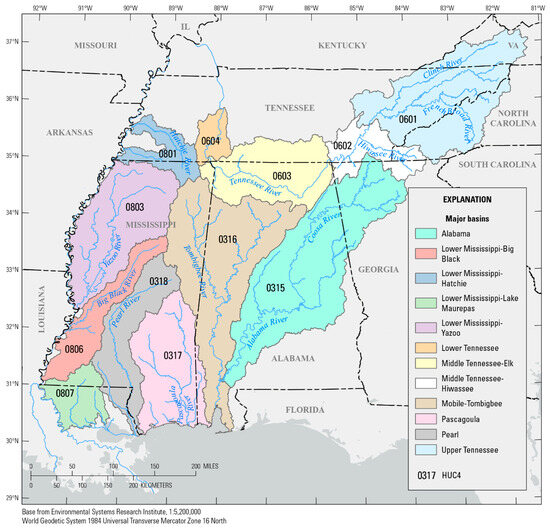
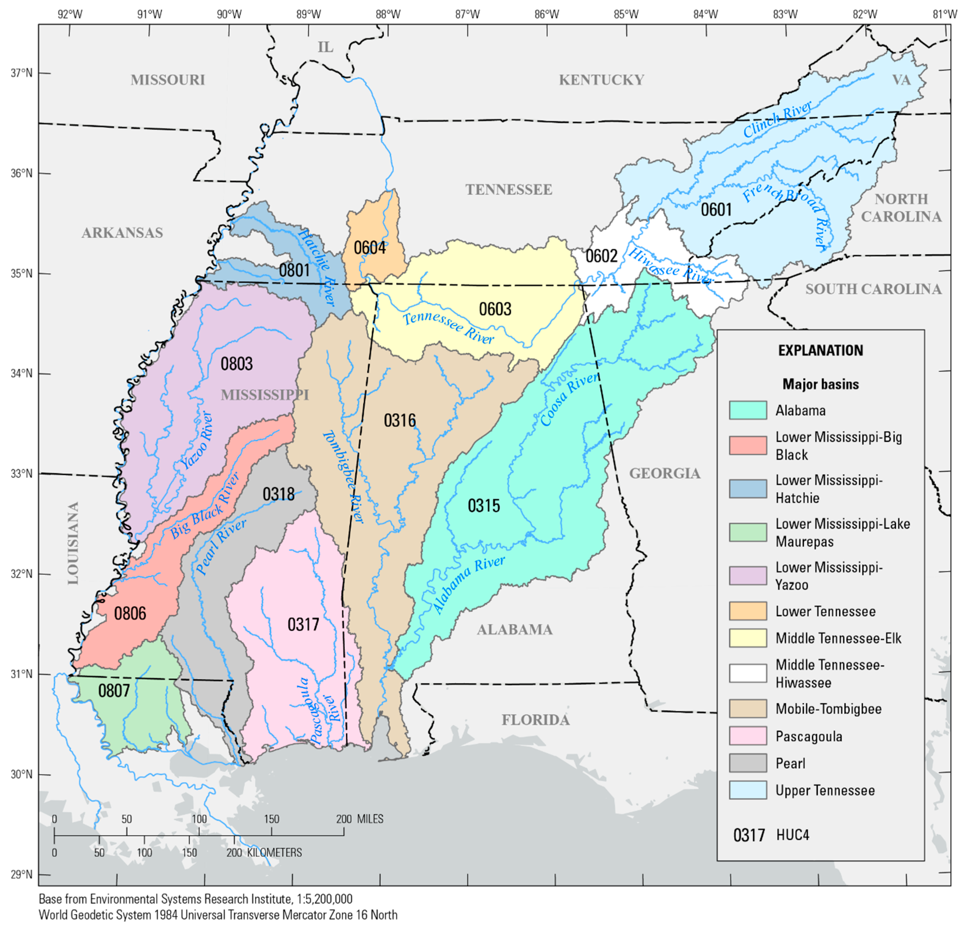
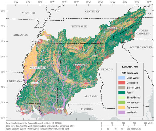
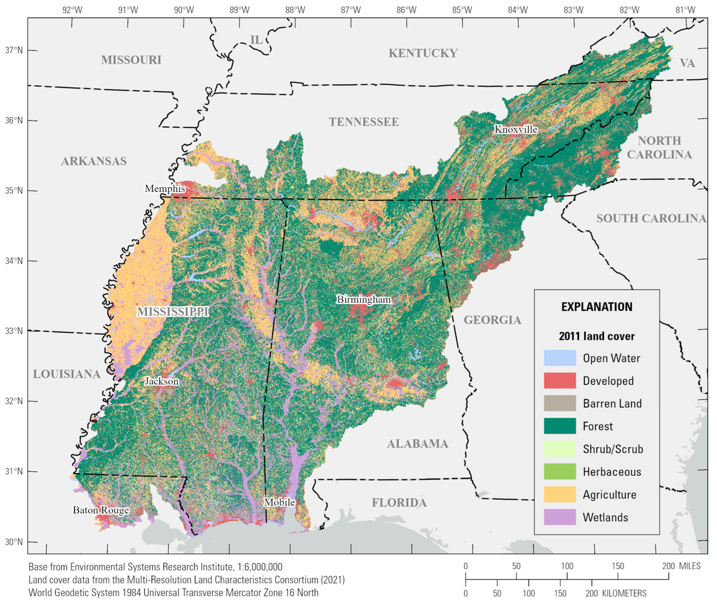
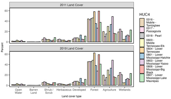
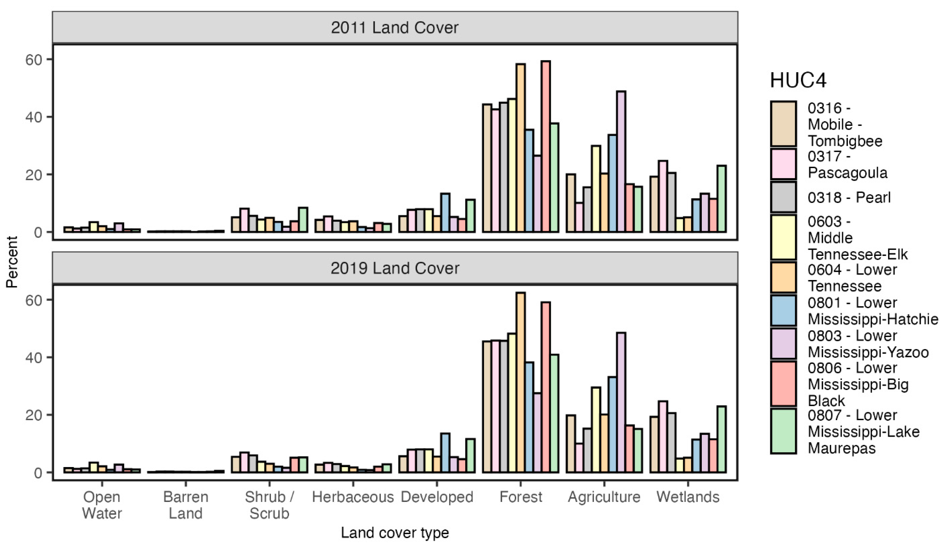
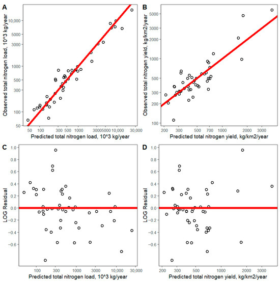
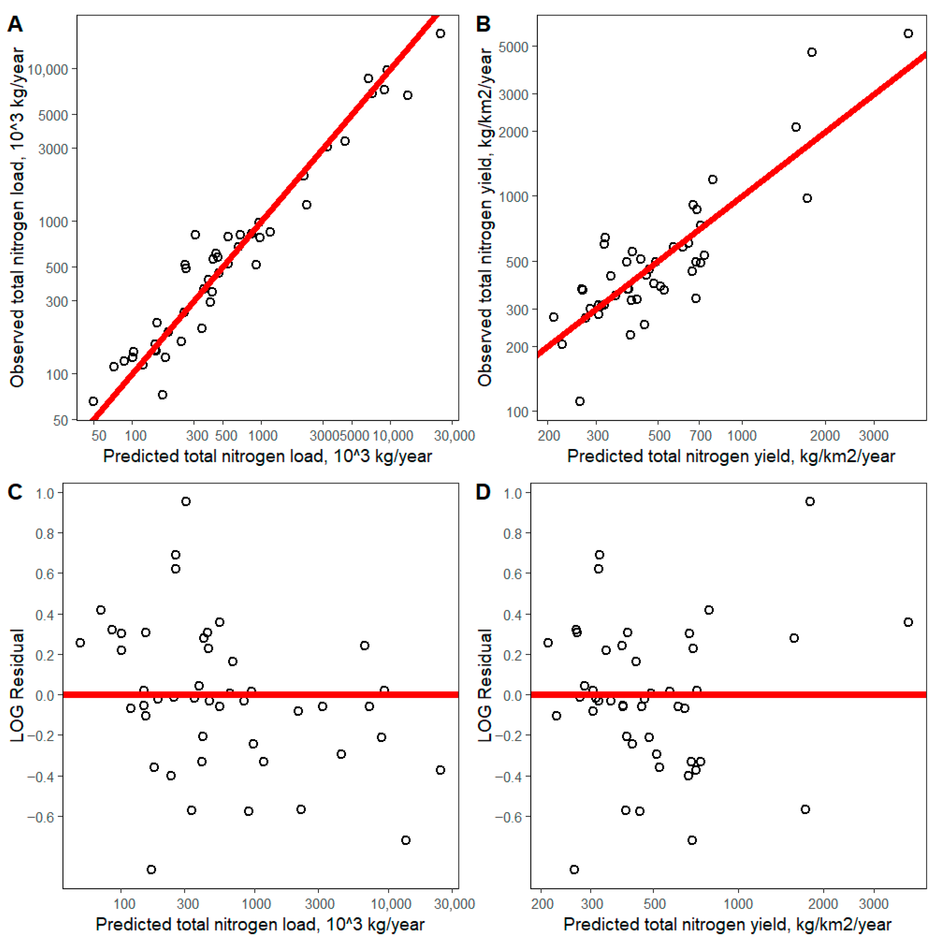
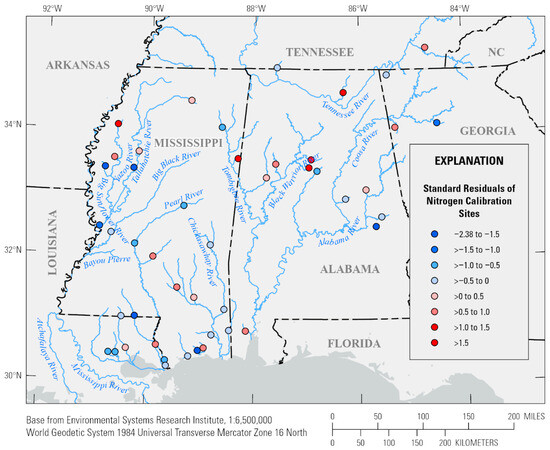
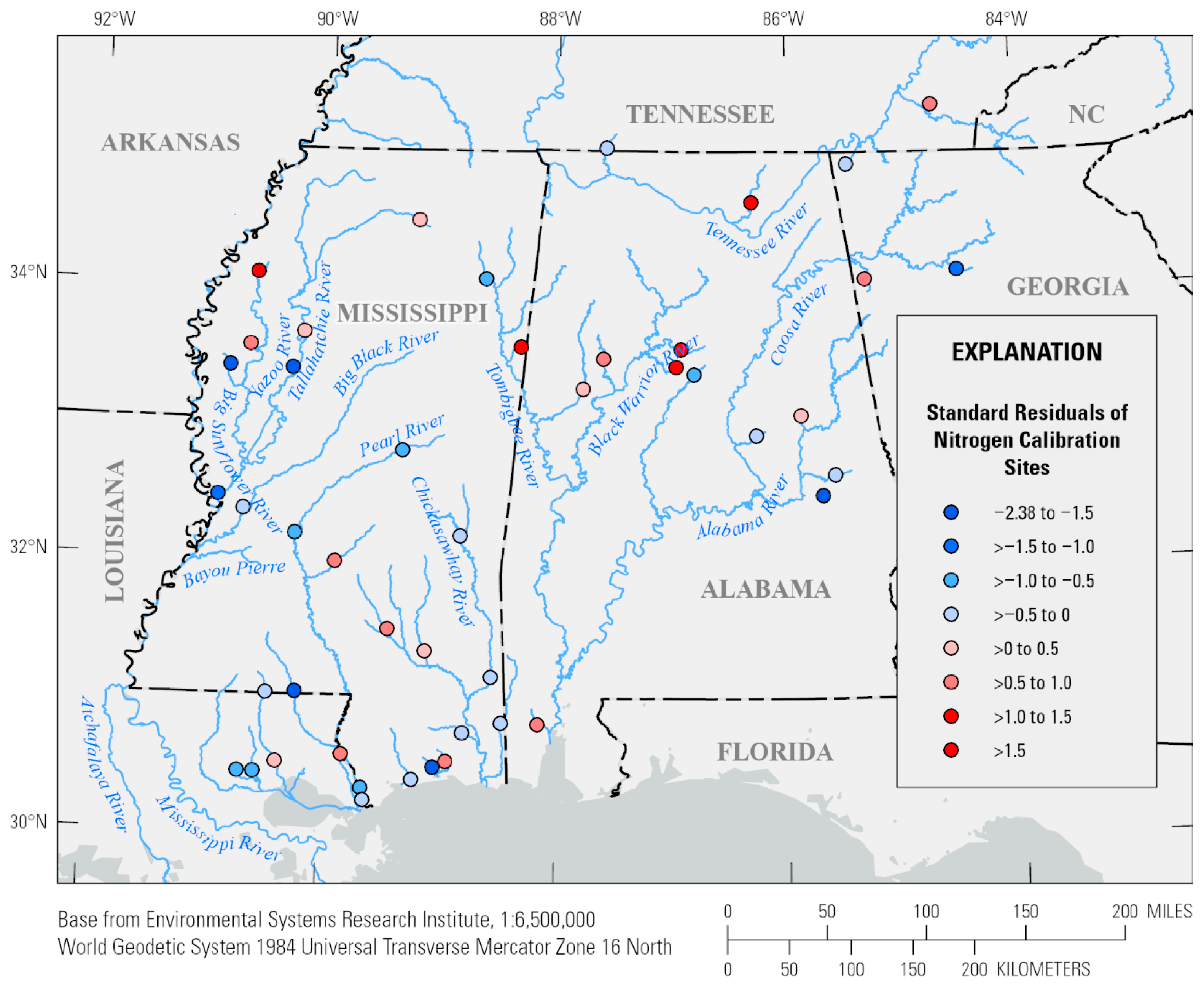
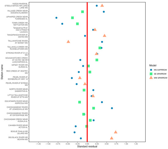
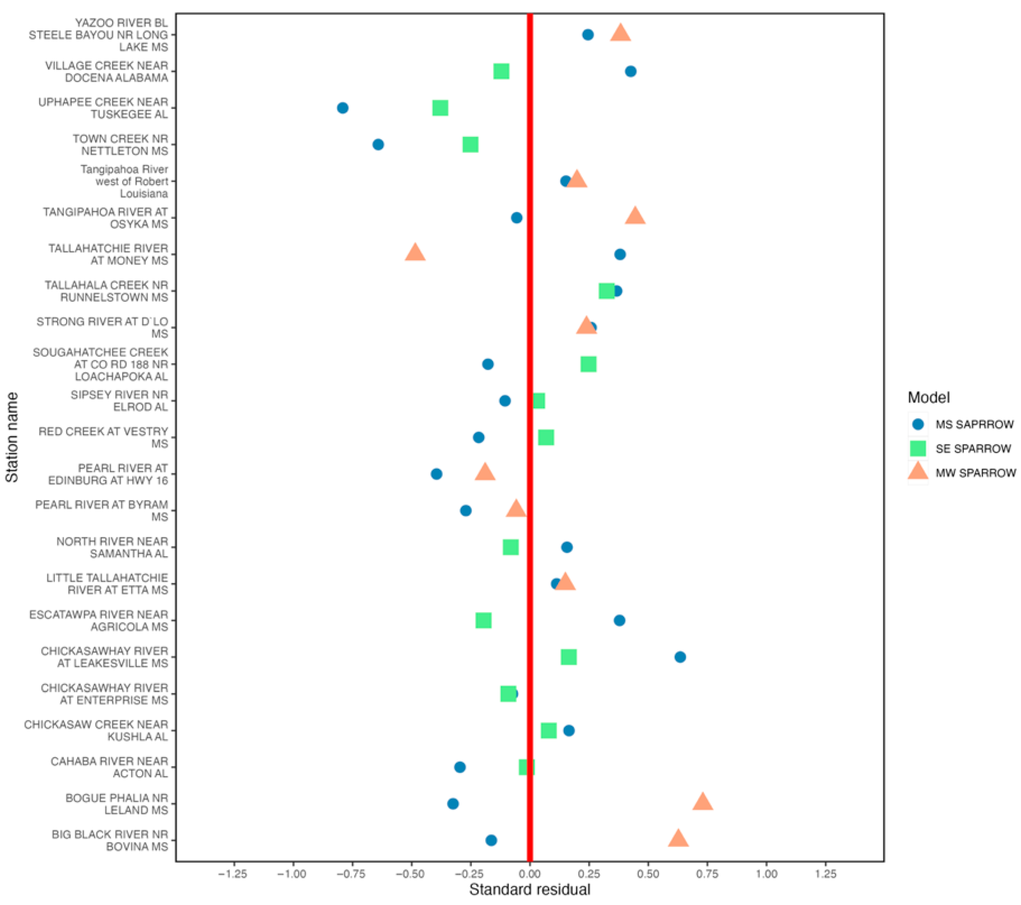
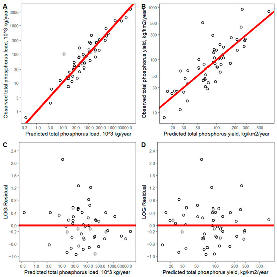
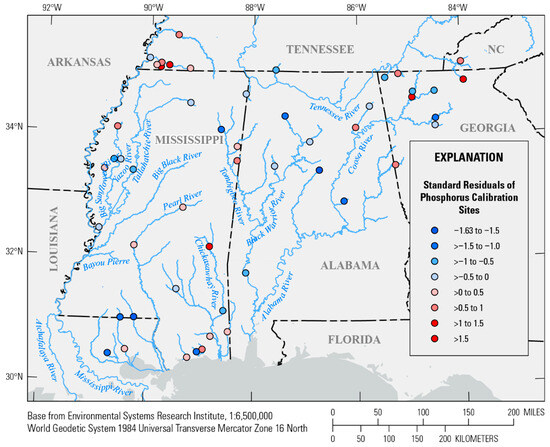
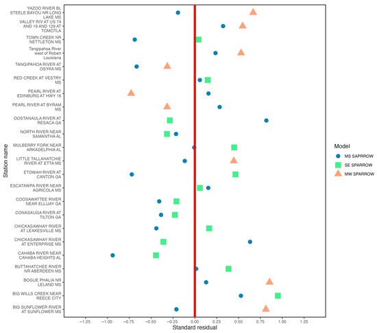
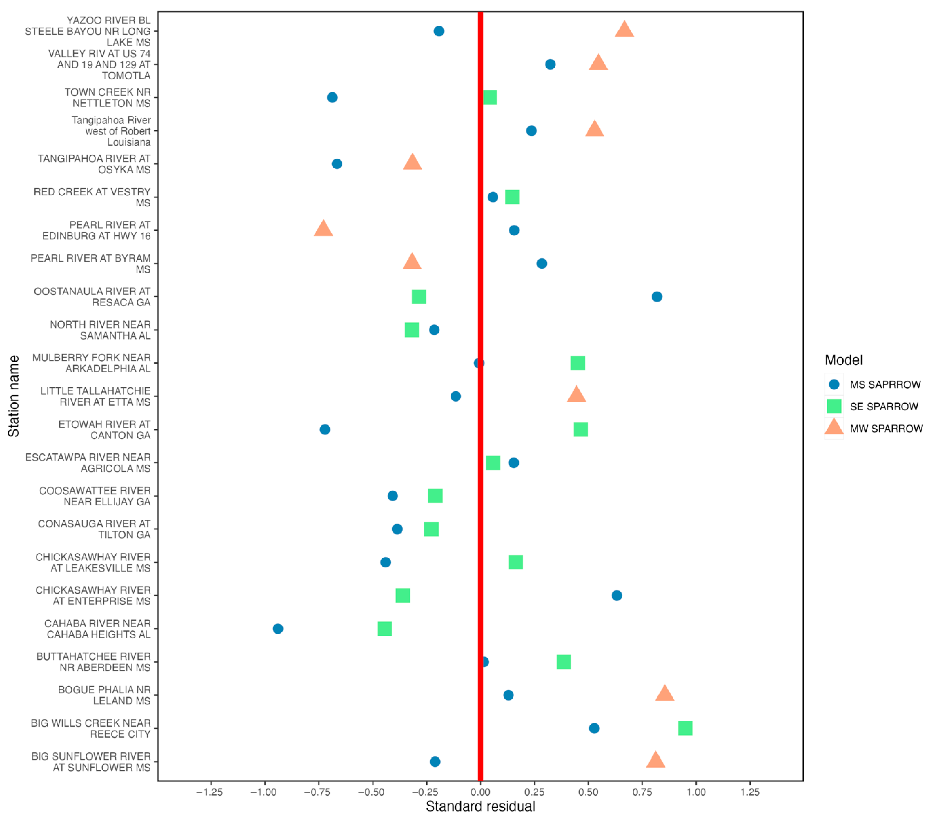
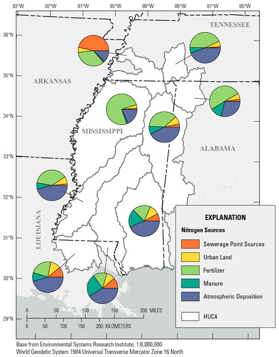
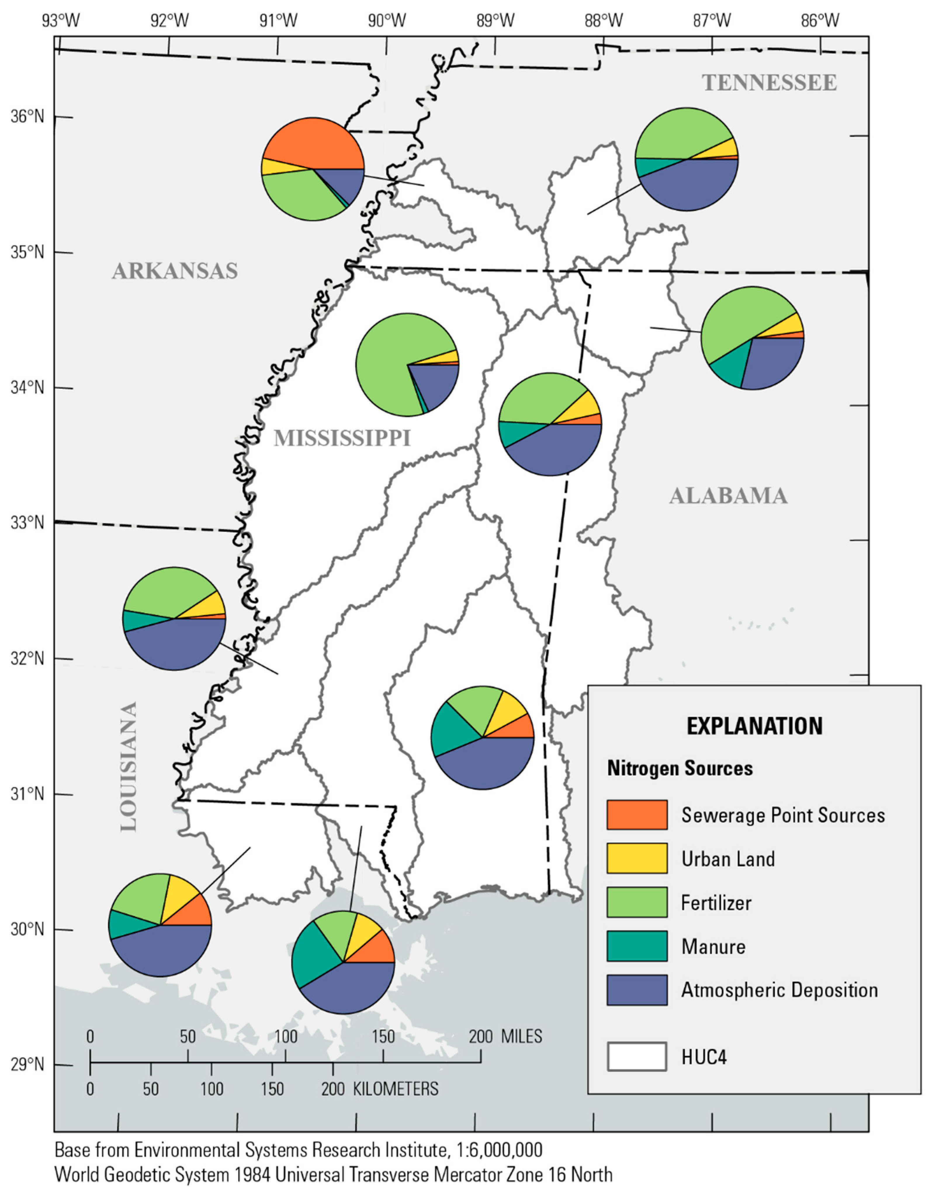
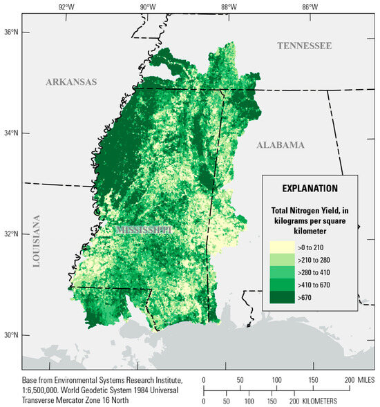
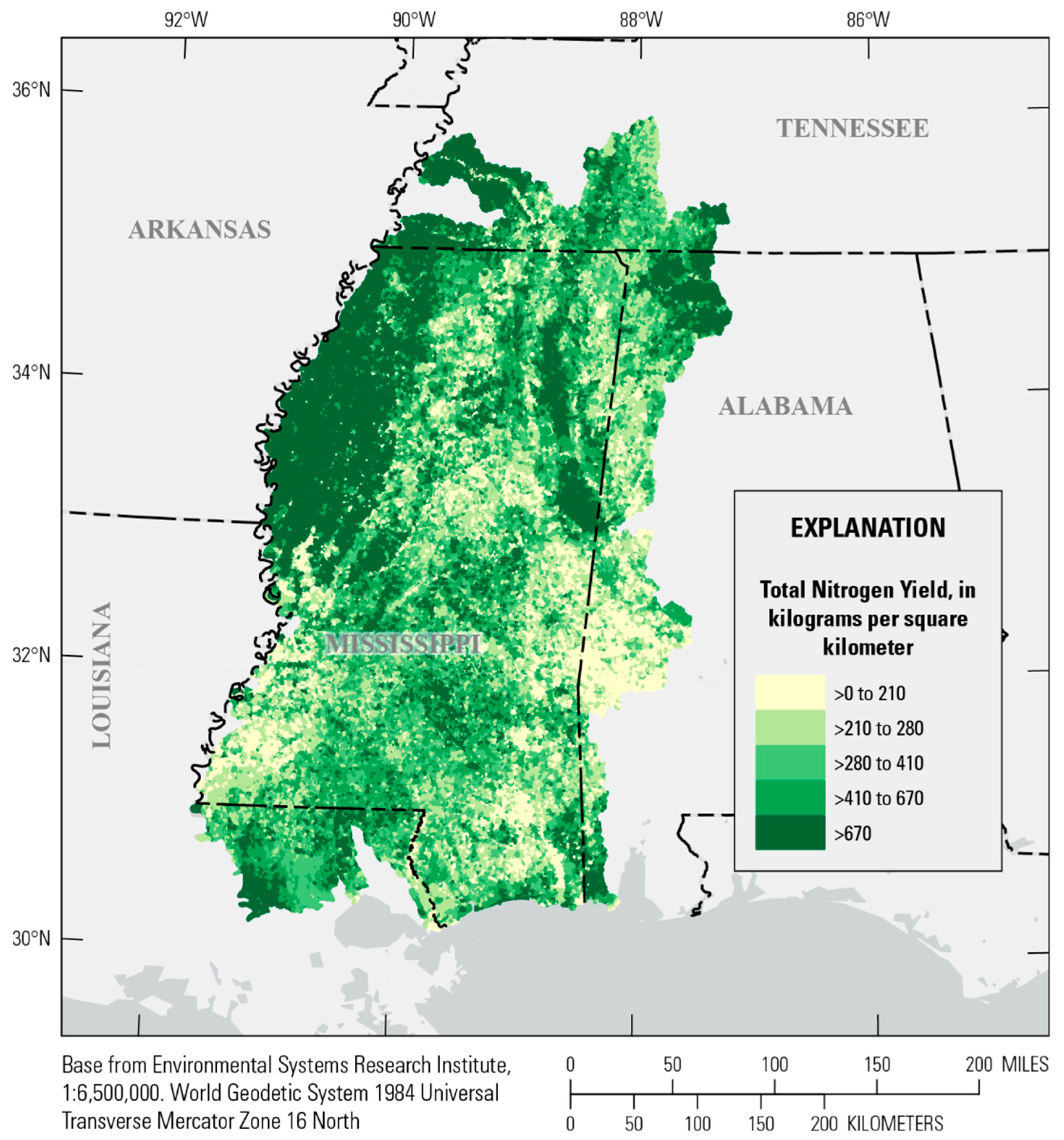
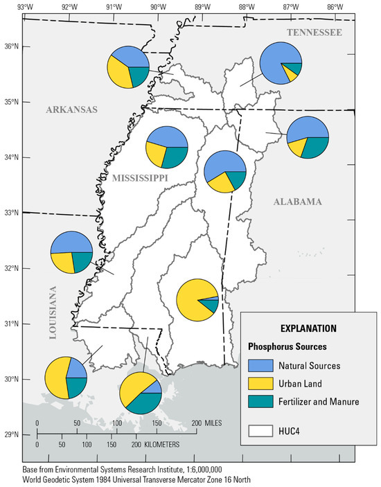
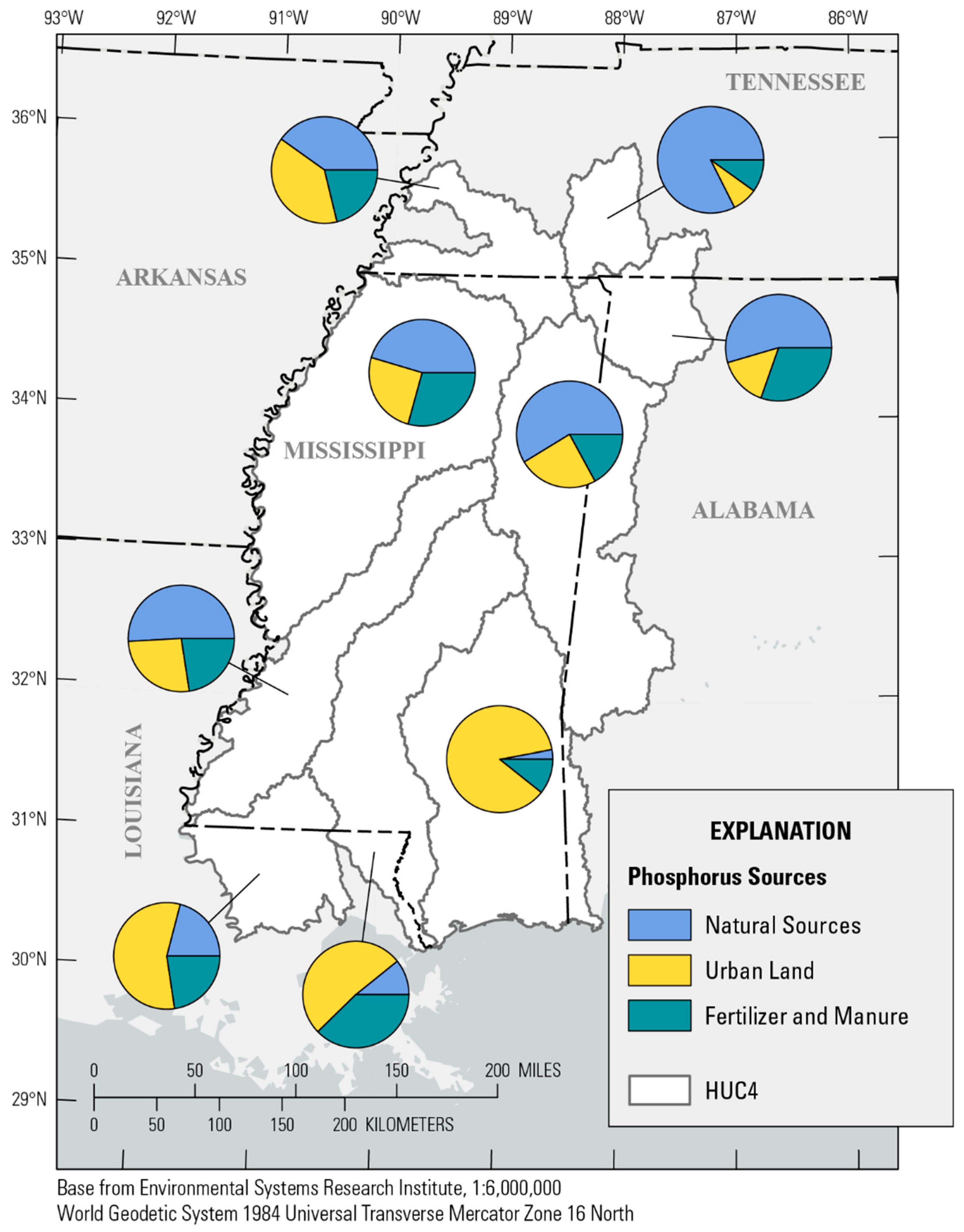
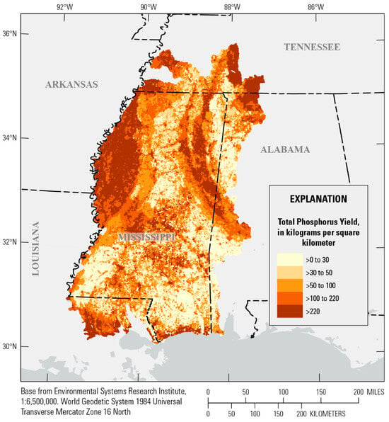
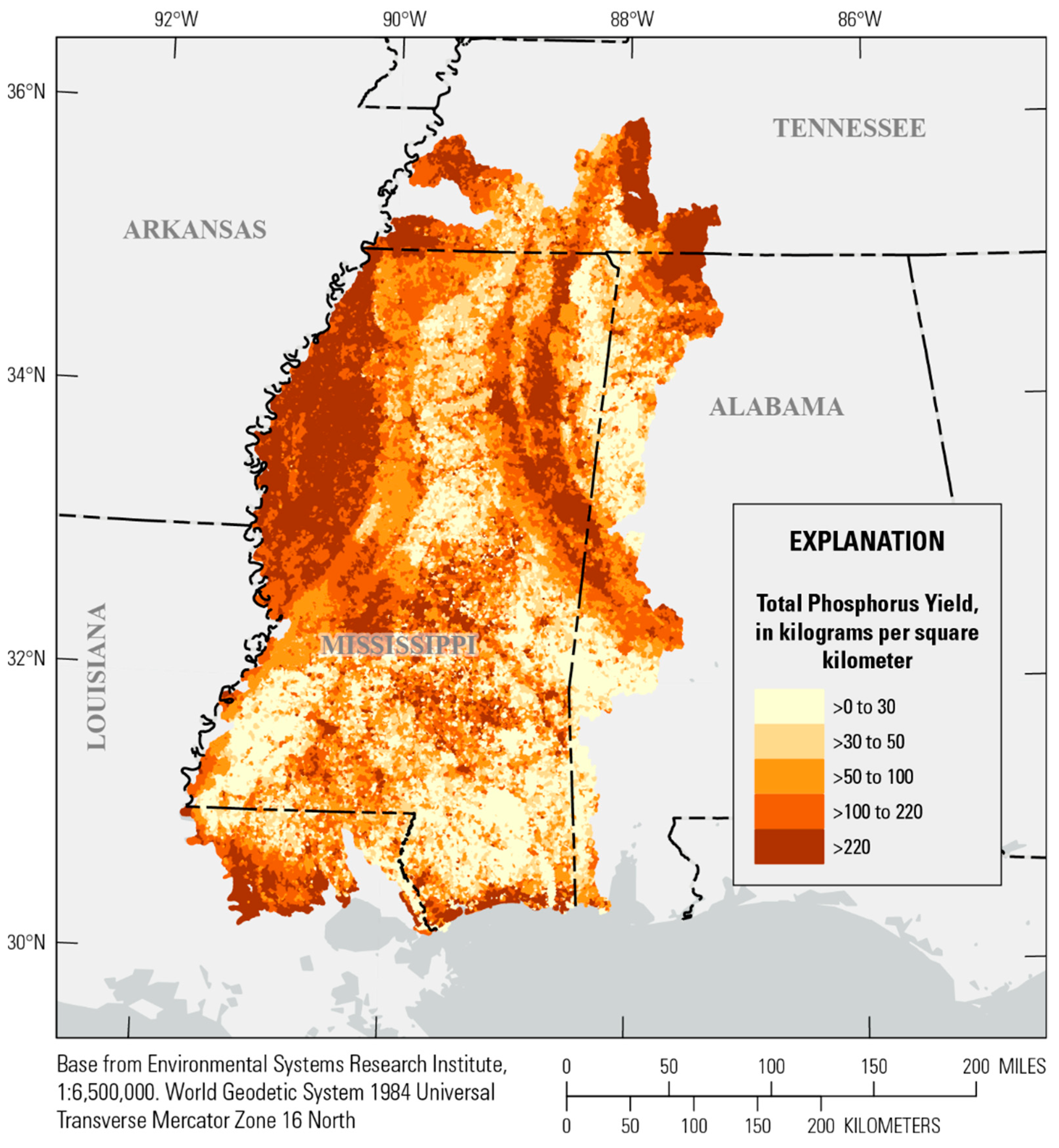
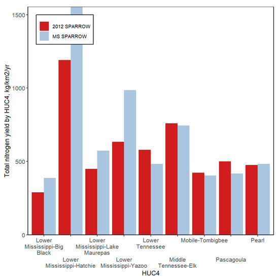
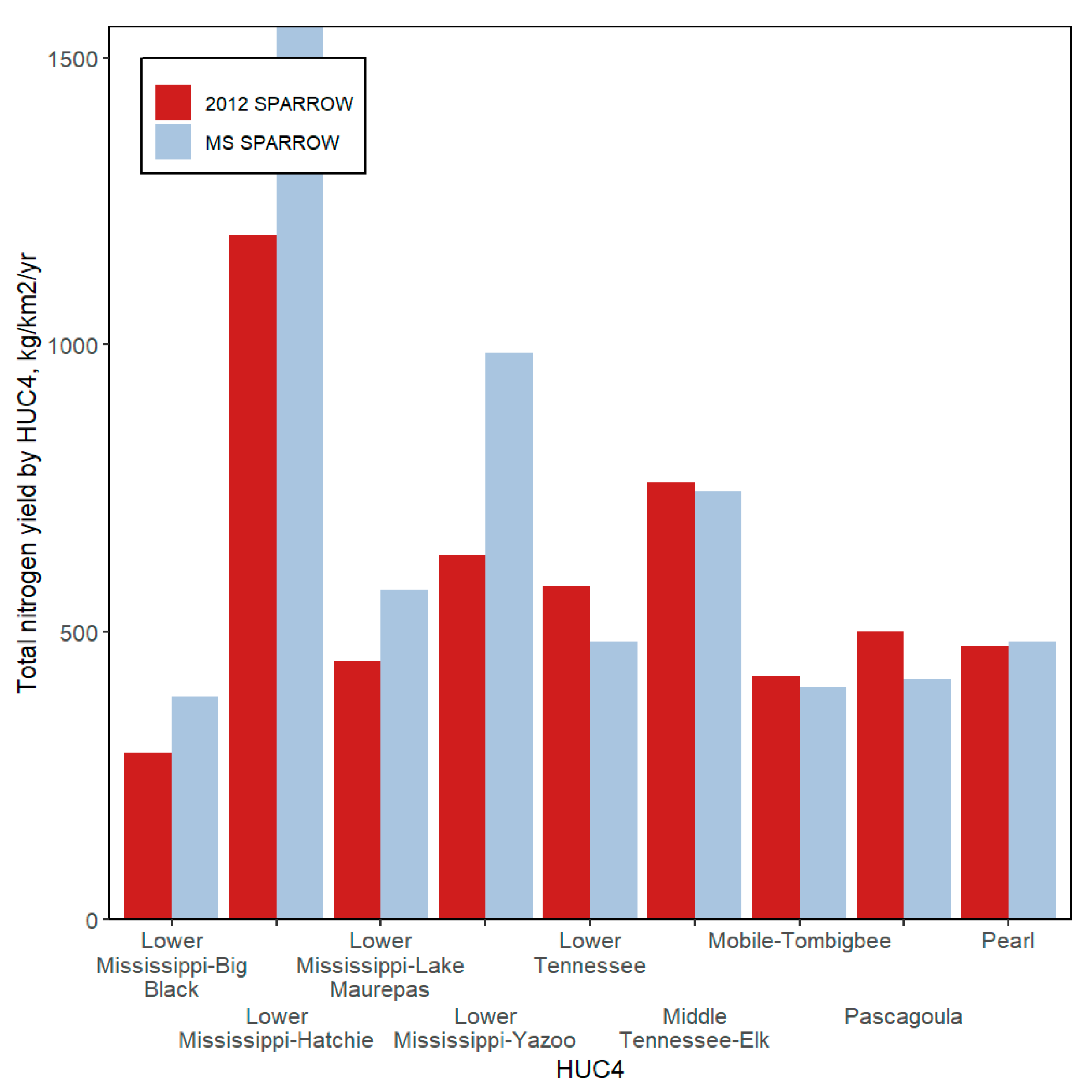
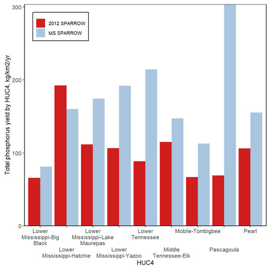
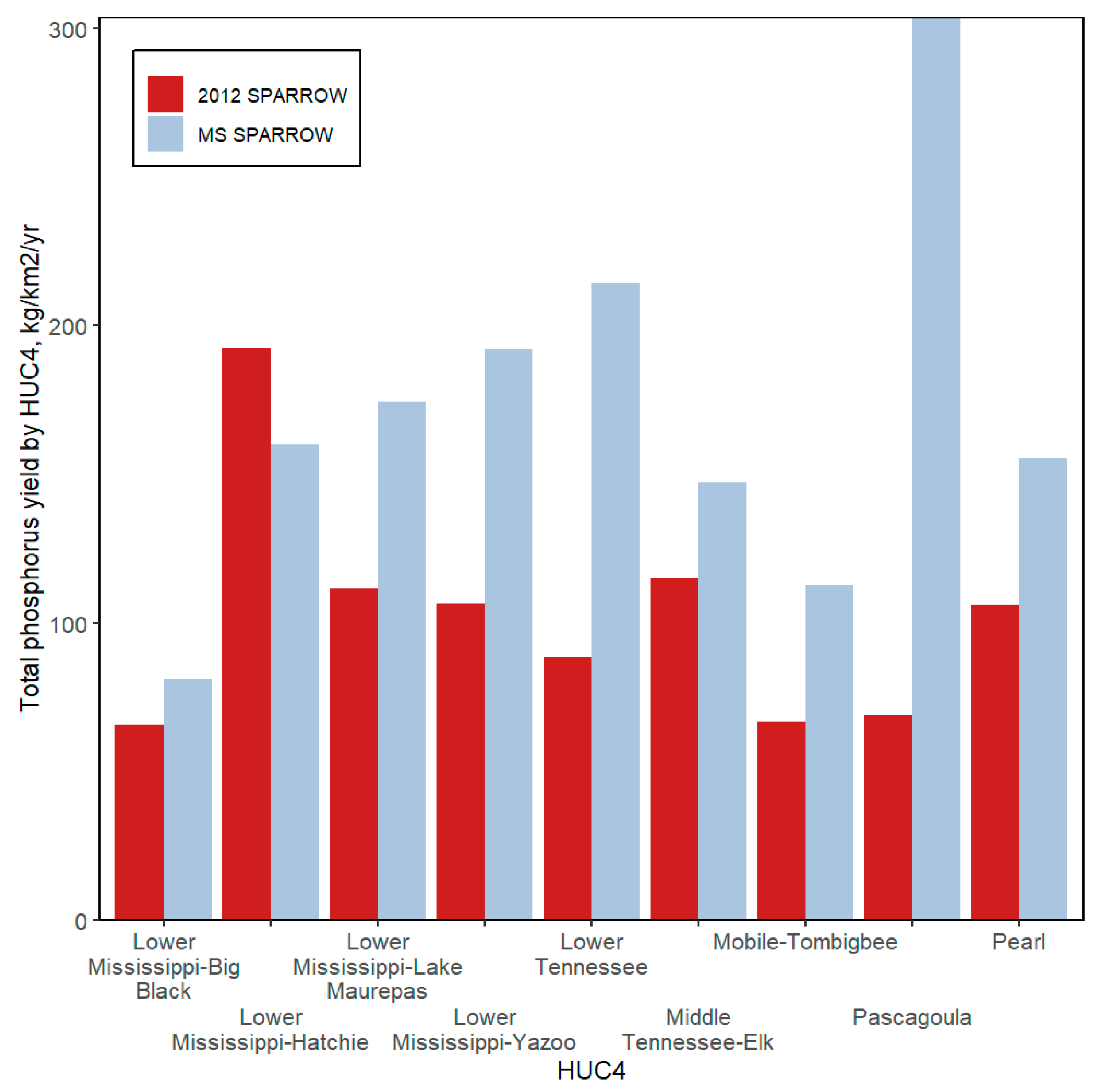

Disclaimer/Publisher’s Note: The statements, opinions and data contained in all publications are solely those of the individual author(s) and contributor(s) and not of MDPI and/or the editor(s). MDPI and/or the editor(s) disclaim responsibility for any injury to people or property resulting from any ideas, methods, instructions or products referred to in the content. |
© 2026 by the authors. Licensee MDPI, Basel, Switzerland. This article is an open access article distributed under the terms and conditions of the Creative Commons Attribution (CC BY) license.